90

Transportation Research Record: Journal of the Transportation Research Board, No. 2283, Transportation Research Board of the National Academies, Washington, D.C., 2012, pp. 90–99.DOI: 10.3141/2283-10

Department of Industrial and Operations Engineering, University of Michigan, 1205 Beal Avenue, Ann Arbor, MI 48109. Corresponding author: L. Yang, youngli@umich.edu.

Different pricing strategies are used to set the toll. The pricing strategy is highly dependent on the objective of the toll lane admin-istrators; that is, if the toll lane is owned by a private company, the administrator might want to maximize the revenue from the toll lane, or if the toll lane is built by the government, the objective might be to minimize the total travel time or to maximize the total throughput. In recent years, research on congestion pricing strategy has received more attention from both academic professionals and practitioners.

The toll pricing scheme can be classified according to the toll col-lection base and rate patterns. Toll collections come in three types: pass based, use based, and distance based. Rate patterns also have three types: flat rate, time-of-day rate, and dynamic rate. The pass-based toll collection scheme issues a toll lane pass to the drivers, and vehicles with a pass can enter the toll lane at any time. It can be either a flat rate or a dynamic rate. With the flat rate, the price of the pass is constant over time, whereas with the dynamic rate, the price of the pass is adjusted month by month. This is the simplest toll collection scheme. However, it is not a good traffic control strategy because once the pass is issued, entry to the toll lane is not restricted for vehicles with a pass, even when the toll lane is almost congested. Therefore, pass-based toll collection is not adaptive and thus not suitable for real-time traffic control.

The other two toll collection schemes, the use-based and distance- based schemes, are more adaptive than the pass-based toll collec-tion scheme. The use-based scheme charges the same price, even though drivers may travel different distances on the toll lane. The distance-based toll scheme charges the drivers a toll on the basis of the distance that they travel, which is more reasonable than the use-based scheme. However, it is also more complicated than the use-based scheme, and determination of the appropriate pricing strategy is difficult. Both use-based and distance-based toll collec-tion schemes can be applied through flat rate, time-of-day rate, and dynamic rate patterns. Table 1, reproduced from the paper of Chung and Recker (3), summarizes the existing high-occupancy toll facilities in the United States and their pricing strategies.

Yang and colleagues investigated pricing schemes for road net-works from the perspective of congestion control (4). They proposed an iterative algorithm that can adjust the toll price on the basis of observation of the link flows over the network without knowledge of the travel time and demand functions or the users’ value of time. Lou et al. also proposed a self-learning approach to determination of a pric-ing strategy for a single toll station on toll lanes and applied a simula-tion to the underlying traffic flow model to determine the prices that optimized an objective (5). Zhang et al. proposed a feedback-based algorithm to adjust toll lane prices dynamically to realize the opti-mal traffic allocation for overall infrastructure efficiency and used a simulation methodology (6).

Distance-Based Dynamic Pricing Strategy for Managed Toll Lanes

Li Yang, Romesh Saigal, and Hao Zhou

Congestion in highway networks inflicts economic and emotional stress on drivers and a considerable cost to society. To mitigate some of these effects, managed toll lanes are being designed and built in the United States. These managed toll lanes guarantee to drivers that they will be able to travel at free-flow speed during peak hours when the gen-eral lanes are congested. The strategy used to price tolls on managed toll lanes has become an important issue; however, few studies have focused on dynamic optimal pricing strategies. This paper formulates the pricing problem on the basis of a stochastic macroscopic traffic flow model and investigates the methodology used to find a pricing strategy to maximize the total expected revenue. A simulation-based numeri-cal algorithm that obtains the optimal prices efficiently in real time is proposed. The methodology is also applicable and readily adjusted for other objective purposes of administrators, such as maximization of total throughput. The general pricing model developed in this paper is not limited to one specific underlying traffic flow model and is read-ily adapted to other macroscopic traffic models, such as the classical Lighthill–Whitham–Richards model.

Just as normal blood circulation necessitates a healthy body, smooth traffic flow is necessary for healthy business and community devel-opment in a city and a region. Traffic congestion haunts cities and communities from various perspectives: it inflicts uncertainties, drains resources, reduces productivity, stresses commuters, and harms the environment. A study by FHWA estimated that 32% of daily travel in major U.S. urban areas occurred under congested traffic conditions (1). In 2009, Schrank and Lomax also showed that congestion caused urban Americans to travel an extra 4.2 billion hours and to purchase an additional 2.8 billion gallons of fuel; thus, incurring a congestion cost of $87.2 billion, an amount more than 50% greater than the costs incurred a decade earlier (2).

Because of the serious impacts of traffic congestion and the con-tinuous deterioration of traffic conditions in urban areas, invest-ments are being made in managed toll lanes in the United States. These provide an alternative way for drivers to avoid congestion. The drivers pay a certain amount of money to enter these toll lanes, and the managed toll lanes guarantee that the drivers will be able to travel at free-flow speed. It not only saves time for the drivers who pay but also decreases the load on congested roads and helps clear the congestion more effectively.

Yang, Saigal, and Zhou 91

To derive the optimal pricing strategy, an underlying traffic flow model is desired. The research described above investigates some problems with dynamic pricing for toll lanes. All the underlying traffic flow models for the pricing schemes are simulation models, but simulation models are more difficult to calibrate and less adap-tive than mathematical models. In this paper, a mathematical model for the dynamic pricing problem based on a sophisticated stochastic traffic flow model is formulated. This model has been validated by Chu et al. (7). The mathematical model can be easily calibrated, and filtering algorithms could also be applied to update the model parameters in real time. The toll pricing problem is formulated as a stochastic optimization problem on the basis of this model. Stochas-tic optimization algorithms are applied to obtain the optimal pricing strategy. An important advantage of this pricing scheme is that it is applicable to toll lanes with any number of toll stations, and the scheme can easily be modified to consider many other objectives.

The objective of this paper is to present the formulation and solution of the dynamic toll pricing problem under the traffic flow dynamics determined by a mathematical model. The next section describes the model formulation, and then the approach used to solve the problem is provided. A numerical example is presented and is followed by conclusions.

Distance-BaseD Dynamic Pricing moDel

Distance-based dynamic pricing is a reasonable and efficient pricing strategy. It is also the most complicated. Although some researchers and practitioners have investigated this pricing strategy in recent years, a unified model for this problem still does not exist. This section introduces a general model for determination of the optimal distance-based tolls.

infrastructure

In the present model, two different kinds of lanes run parallel. One is a general lane that drivers can enter for free. The other is a man-aged toll lane that drivers must pay a toll to enter. During peak hours, the general lane is normally congested and the toll lane is maintained at free-flow speed by adjustment of the toll prices. This is useful for drivers who can pay a toll to avoid congestion as well as in emergency situations.

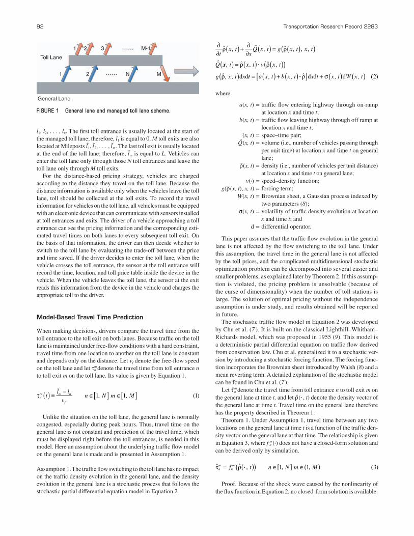
Figure 1 illustrates the structure of the managed toll lane and the general lane in this model. Suppose that the managed toll lane starts at Milepost 0 and ends at Milepost L. N toll entrances are located at

TABLE 1 Overview of High-Occupancy Toll Facilities in the United States

Location HOT Configuration Toll Policy Toll Pattern and Range

I-15, Salt Lake City, Utah 45.6 mi, 2 lanes. Midway accessible. 8 general lanes.

HOV2+:free.SOV: tolled

Monthly pass: $50 per month

US-290, Houston, Tex. 14 mi, reversible, 1 lane. Midway inaccessible. 8 general lanes.

Peak (HOT lane)HOV3+: freeHOV2: tolledSOV: prohibited

Off peak (HOV2+ lane) HOV2+: freeSOV: prohibited

Flat rate: $2 per use

SR-91, Orange County, Calif. 10 mi, 4 lanes. Midway inaccessible. 8 general lanes.

PeakHOV3+: 50% toll offHOV2, SOV: fully tolled

Off peakHOV3+: freeHOV2, SOV: fully tolled

Time-of-day tolls: $1.25–9.55 per use

I-25, Denver, Colo. 6.6 mi, reversible, 2 lanes. Midway inaccessible. 8 general lanes.

HOV2+: freeSOV: tolled

Time-of-day tolls: $0.50–3.50 per use

I-10W, Houston, Tex. 12 mi, 4 lanes. Midway accessible. 10 general lanes.

Bus: freeHOV2+: peak free; off

peak tolledSOV: tolled

Time-of-day tolls by distance: $0.30–1.60 per toll section

I-15S, San Diego, Calif. 8 mi, reversible, 2 lanes. Midway inaccessible. 10 general lanes.

HOV2+: freeSOV: tolled

Dynamic tolls: $0.50– 8.00 per use

I-95, Miami, Fla. 7.75 mi, 4 lanes. Midway inaccessible. 8 general lanes.

HOV3+: freeHOV2, SOV: tolled

Dynamic tolls: $0.25–7.25 per use

SR-167, Seattle, Wash. 9 mi, 2 lanes. Midway accessible. 4 general lanes.

HOV2+: freeSOV: tolled

Dynamic tolls: $0.50– 9.00 per use

I-15N, San Diego, Calif. 12 mi, reversible, 4 lanes. Midway accessible. 8 general lanes.

HOV2+: freeSOV: tolled

Dynamic tolls by distance: $0.50–8.00

I-394, Minneapolis, Minn. 7 mi, 2 lanes, and 3.3 mi, reversible, 2 lanes. 2 tolling sections. Midway accessible. 4 general lanes.

HOV2+: freeSOV: tolled

Dynamic tolls by distance: $0.25–8.00

Note: HOT = high-occupancy toll; HOV = high-occupancy vehicle; SOV = single-occupancy vehicle.

92 Transportation Research Record 2283

l1, l2, . . . , ln. The first toll entrance is usually located at the start of the managed toll lane; therefore, l1 is equal to 0. M toll exits are also located at Mileposts l̃1, l̃2, . . . , l̃m. The last toll exit is usually located at the end of the toll lane; therefore, l̃m is equal to L. Vehicles can enter the toll lane only through those N toll entrances and leave the toll lane only through M toll exits.

For the distance-based pricing strategy, vehicles are charged according to the distance they travel on the toll lane. Because the distance information is available only when the vehicles leave the toll lane, toll should be collected at the toll exits. To record the travel information for vehicles on the toll lane, all vehicles must be equipped with an electronic device that can communicate with sensors installed at toll entrances and exits. The driver of a vehicle approaching a toll entrance can see the pricing information and the corresponding esti-mated travel times on both lanes to every subsequent toll exit. On the basis of that information, the driver can then decide whether to switch to the toll lane by evaluating the trade-off between the price and time saved. If the driver decides to enter the toll lane, when the vehicle crosses the toll entrance, the sensor at the toll entrance will record the time, location, and toll price table inside the device in the vehicle. When the vehicle leaves the toll lane, the sensor at the exit reads this information from the device in the vehicle and charges the appropriate toll to the driver.

model-Based travel time Prediction

When making decisions, drivers compare the travel time from the toll entrance to the toll exit on both lanes. Because traffic on the toll lane is maintained under free-flow conditions with a hard constraint, travel time from one location to another on the toll lane is constant and depends only on the distance. Let vf denote the free-flow speed on the toll lane and let τm

n denote the travel time from toll entrance n to toll exit m on the toll lane. Its value is given by Equation 1.

τnm m n

f

tl l

vn N m M( ) ≡ − ∈[ ] ∈[ ]

1 1 1, , ( )

Unlike the situation on the toll lane, the general lane is normally congested, especially during peak hours. Thus, travel time on the general lane is not constant and prediction of the travel time, which must be displayed right before the toll entrances, is needed in this model. Here an assumption about the underlying traffic flow model on the general lane is made and is presented in Assumption 1.

Assumption 1. The traffic flow switching to the toll lane has no impact on the traffic density evolution in the general lane, and the density evolution in the general lane is a stochastic process that follows the stochastic partial differential equation model in Equation 2.

∂∂

( ) + ∂∂

( ) = ( )( )t

x tx

Q x t g x t x t

Q

ˆ , ˆ , ˆ , , ,

ˆ

ρ ρ

xx t x t v x t

g x t x

, ˆ , ˆ ,

ˆ, ,

( ) = ( ) ( )( )( )

ρ ρ

ρ

i

d dtt a x t b x t x t x t W x t= ( ) + ( )[ ] + ( ) ( ), , ˆ , ,i ρ σd d d (( )2

where

a(x, t) = traffic flow entering highway through on-ramp at location x and time t;

b(x, t) = traffic flow leaving highway through off ramp at location x and time t;

(x, t) = space–time pair; Q̂(x, t) = volume (i.e., number of vehicles passing through

per unit time) at location x and time t on general lane;

ρ̂(x, t) = density (i.e., number of vehicles per unit distance) at location x and time t on general lane;

v(i) = speed–density function; g(ρ̂(x, t), x, t) = forcing term; W(x, t) = Brownian sheet, a Gaussian process indexed by

two parameters (8); σ(x, t) = volatility of traffic density evolution at location

x and time t; and d = differential operator.

This paper assumes that the traffic flow evolution in the general lane is not affected by the flow switching to the toll lane. Under this assumption, the travel time in the general lane is not affected by the toll prices, and the complicated multidimensional stochastic optimization problem can be decomposed into several easier and smaller problems, as explained later by Theorem 2. If this assump-tion is violated, the pricing problem is unsolvable (because of the curse of dimensionality) when the number of toll stations is large. The solution of optimal pricing without the independence assumption is under study, and results obtained will be reported in future.

The stochastic traffic flow model in Equation 2 was developed by Chu et al. (7 ). It is built on the classical Lighthill–Whitham–Richards model, which was proposed in 1955 (9). This model is a deterministic partial differential equation on traffic flow derived from conservation law. Chu et al. generalized it to a stochastic ver-sion by introducing a stochastic forcing function. The forcing func-tion incorporates the Brownian sheet introduced by Walsh (8) and a mean reverting term. A detailed explanation of the stochastic model can be found in Chu et al. (7 ).

Let τ̃ mn denote the travel time from toll entrance n to toll exit m on

the general lane at time t, and let ρ̂(i , t) denote the density vector of the general lane at time t. Travel time on the general lane therefore has the property described in Theorem 1.

Theorem 1. Under Assumption 1, travel time between any two locations on the general lane at time t is a function of the traffic den-sity vector on the general lane at that time. The relationship is given in Equation 3, where f mn (i) does not have a closed-form solution and can be derived only by simulation.

ˆ ˆ , , , ( )τ ρnm

nmf t n N m M= ( )( ) ∈[ ] ∈( )i 1 1 3

Proof. Because of the shock wave caused by the nonlinearity of the flux function in Equation 2, no closed-form solution is available.

FIGURE 1 General lane and managed toll lane scheme.

1 2 3 M-1

1 2 N

General Lane

Toll Lane

M

Yang, Saigal, and Zhou 93

Therefore, finite difference schemes are used to solve it numeri-cally and obtain approximate solutions. However, because of shock waves, any simple finite difference scheme will fail to solve the stochastic partial differential equation because the solution is generally discontinuous. Godunov’s scheme is a numerical method that can handle this difficulty and give a high-resolution solution to homogeneous conservation law (10). The present stochastic model is a nonhomogeneous conservation law because of the forcing term g(ρ̂(x, t), x, t). Leveque has developed a modified Godunov scheme in which the forcing terms can be incorporated into the scheme (11). ◾

In Model 2, the forcing term g(ρ̂(x, t), x, t) is a stochastic func-tion, so the evolution of ρ̂ is also stochastic. Simulation is used to obtain the travel time function f mn (i) in two stages. In Stage 1, a number of scenarios are simulated and the density evolution under each scenario is generated. In Stage 2, after the density evolution is generated, travel time can be calculated under each scenario via the speed–density function and the average travel time over all scenarios is considered the prediction of the travel time.

The steps used to obtain the density evolution in Stage 1 by the modified Godunov scheme are described below. For a detailed explanation, refer to Leveque’s paper (11).

Step 1. Simulate a number of Brownian sheets for each scenario according to the numerical generation algorithm (8).

Step 2. Divide the highway into small cells with length Δx and discretize the time by Δt. Let ρ̂j

i denote the average density on the general lane over cell i at time t + jΔt. When j is equal to 0, obtain the initial condition for ρ̂0

i according to Equation 4, where ρ̂(i , t) represents the initial density vector on the general lane at time t.

ˆ ˆ , ( )ρ ρii

i

xx

x t x0

1

4= ( )−

∫ d

Step 3. Each cell is divided into two segments. Let ρ̂ij,− denote

the average value of the density in the upstream segment of cell i, and let ρ̂i

j,+ denote the average value of density in the downstream segment of cell i. Obtain the values with the following equations:

ˆ ˆ ˆ ( )

ˆ ˆ

, ,

, ,

ρ ρ ρ

ρ ρ

ij

ij

ij

ij

ijQ Q g

− +

+ −

+ =

( ) − ( ) =

2 5

ˆ̂ , ,ρij

i ix t x( )∆

Step 4. Let ρ̂ji−0.5 and ρ̂j

i+0.5 denote the average value of density over time interval [tj, tj+1] at the left boundary and the right boundary of cell i, respectively. The value of ρ̂j

i+0.5 can be obtained according to the solution of the Riemann problem (12). Define a Riemann problem with the following initial condition that jumps from ρ̂i

j,+ to ρ̂j,−

i+1 at location xi+0.5.

ˆ

ˆ ˆ ˆ ,

ˆ

.

, , ,

ρ

ρ ρ ρ

ρ

ij

ij

ij

ij

ij

s

+

+ ++−

+

=

< >

0 5

1

1

0if

,, , ,

, ,

ˆ ˆ ,

ˆ ˆ ˆ

− ++−

++−

< <

<

if

if

ρ ρ

ρ ρ

ij

ij

ij

ij

s1

1

0

ρρ

ρ

ij

ij

Q

Q Q

,

,

,

ˆ ˆ

+ −

−+− −

< ′ ( )′ ( ) < ′ ( ) <

1

11

1

0

0 0if ρρ

ρ ρ ρ

ij

ij

ij

ijQ

,

, , ,ˆ ˆ ˆ

+

+− −

+− +′ ( ) < <

11

10if

( )6

where

sQ Qi

jij

ij

ij

=( ) + ( )

−

++−

++−

ˆ ˆ

ˆ ˆ

, ,

, ,

ρ ρρ ρ

1

1

Step 5. Update the state variables for the next time interval according to Equation 7. The state variables in the next time interval are also averaged over each cell and become a piecewise constant approximation. After the update, make j equal to j + 1 and then go back to Step 2.

ˆ ˆ ˆ ˆ ˆ,. .ρ ρ ρ ρ ρi

jij

ij

ijt

xQ Q g+

− += + ∆∆

( ) − ( ) +0 5 0 5 iij

i jx t x, , ( )( )∆ 7

After a number of scenarios and the density evolution under each scenario are generated, the steps used to obtain the travel time function in Stage 2 are described below.

Step 1. Let Tk(x) denote the arrival time of location x on the general lane under scenario k, given that the vehicle is at location ln at time t.

Step 2. Solve the following differential equation numerically by discretization of the time and space to obtain T k(l̂m) which is the arrival time of location l̂m. The travel time from ln to l̂m under scenario k is then T k(l̂m) − T k(ln).

dd

Tx

v x T

T l t

k

k k

kn

= ( )( )( ) =

ˆ ,( )

ρ8

Step 3. Take the average of Tk(l̂m) − T k(ln) as the predicted travel time from ln to l̂m. The value of f mn (i) is then obtained.

On the basis of the explanation presented above, function f mn (i) is complicated and can be obtained only through simulation. How-ever, the complexity of the travel time function does not affect the pricing model. For any traffic flow model, as long as the travel time can be expressed as a function of the density vector, the pricing model and the methodology described here apply.

Demand Function

For every toll entrance, the traffic demand can be classified by the destination. For example, for toll entrance n, let Φn denote the set of indexes of all toll exits behind toll entrance n. Let Dn(t) denote the traffic entering the toll lane through toll entrance n at time t. It consists of Dm

n (t) (m ∈ Φn), where Dmn (t) represents the traffic enter-

ing at toll entrance n at time t and destined to leave at toll exit m. Equation 9 describes this relationship.

D t D tn nm

m n

( ) = ( )∈∑

Φ

( )9

At time t, the toll entrance n publishes the prices for every down-stream exit as well as the corresponding estimated travel times in both the general lane and the toll lane. On the basis of this information, the drivers decide whether to stay in the general lane or switch to the toll lane. Let pm

n (t) denote the toll for entry at entrance n at time t and departure at exit m. The demand function is given in Equation 10.

94 Transportation Research Record 2283

D t p t t tnm

nm

nm

nm

nm( ) = ( ) ( ) ( )( )d , ˆ , ( )τ τ 10

Little information on the modeling of the demand function is available in the literature. Lou et al. proposed use of a logit model for the demand function (5). The logit model is widely used to model the demand function with alternative choices. Equation 11 describes the basic idea of a logit model, in which D is the realized traffic demand for the toll lane, A is the potential total demand, Uh is the utility of the choice of the toll lane, and Ug is the utility of the choice of the general lane.

D AU

U U

h

h g=

( )( ) + ( )

exp

exp exp( )11

Lou et al. assume that the utility functions follow Equation 12, where τ and τ̂ are the travel times on the toll lane and general lane, respectively, from the driver’s origin to destination; p is the toll price for the driver’s travel distance (5). α, η, γ h, and γ g are param-eters. It should be noted that α and η are less than 0 because the utility function is decreasing in the travel time and toll price. This utility function is used in the model described here.

U p

U

h h

g g

= − − +

= − +

ατ η γ

ατ γˆ( )12

When Equation 12 is plugged into Equation 11, the demand func-tion is obtained in Equation 13. Thus, the traffic volume entering the toll lane is related to the time saved and toll price.

D Ap

g h

=+ −( ) + +( )

= −

1

113

exp ˆ( )

α τ τ η γ

γ γ γ

The traffic demand for each origin–destination pair is assumed to follow the logit model and is given in Equation 14. In Equation 14, Am

n (t), α mn , ηmn , and γ mn are the parameters for the origin– destination

pair consisting of toll entrance n and toll exit m. These parameters can be calibrated by use of the reactive self-learning algorithm developed by Lou et al. (5).

D t A tt t pn

mnm

nm

nm

nm

nm( ) = ( )

+ ( ) − ( )( ) +1

1 exp ˆα τ τ η nnm

nmt( ) +( )γ

( )14

constraint

In the present model, maintenance of free-flow speed on the toll lane is a hard constraint, and the toll prices are adjusted dynami-cally to make sure that this constraint is not violated. However, in practice, this constraint might be violated because of sudden spike in demand. Once this situation happens, the pricing strategy will be switched to another mode under which all the toll prices will be set to the maximum price or the toll lane will even be temporarily closed until the managed toll lane again recovers to the free-flow speed condition. The maximum price is usually predetermined by an agreement between the public and highway administrators and serves as an upper threshold for the toll prices.

The main focus in this paper is the pricing strategy used when this constraint is not violated. Therefore, the authors consider retention of the toll lane congestion being free as a hard constraint. In other words, the traffic on the toll lane must travel at the free-flow speed. To satisfy this constraint, the traffic flow entering the toll lane cannot affect the existing traffic on the toll lane. Every lane has a traffic flow capacity. It is assumed that if the flow does not exceed this capacity, then free-flow speed is attained. Such a constraint can be mathematically described in Equation 15, where Cn is the flow capacity on the toll lane for toll entrance n. At time t, qn(t) is the incoming total traffic flow on the toll lane right before toll entrance n. The constraint guarantees that the total flow after every toll station will not exceed the flow capacity of the toll lane. qn(t) consists of q mn (t), where q mn (t) represents the traffic volume whose destination is toll exit m among traffic flow qn(t).

qn t q t n N

D t C q t n

nm

m

n n n

n

( ) = ( ) ∀ ∈[ ]

( ) ≤ − ( ) ∀ ∈

∈∑

Φ

1,

11

15

,

( )

N[ ]

Another constraint is for the flow conservation on the toll lane. Let κn denote the travel time between toll entrance n and toll entrance n + 1 on the toll lane. Because the toll lane is under free-flow speed vf, κn is given in Equation 16.

κnn n

f

l l

v= −+1 16( )

The vehicles passing toll entrance n at time t will arrive at toll entrance n + 1 at time t + κn; therefore, q mn (t) will follow Equa-tion 17. qm

1 (t) is 0, as the first toll entrance is assumed to be located at the beginning of the toll lane.

q t m

q t q t D

m

nm

nm

n nm

1 1

1 1 1

0 17( ) = ∀ ∈

( ) = −( ) +− − −

Φ ( )

κ tt n N mn n−( ) ∀ ∈[ ] ∈−κ 1 2, , Φ

complete model Formulation

The objective of the pricing strategy is to maximize the total revenue from time T0 to time t. When the information presented above is combined, the complete model of distance-based dynamic pricing is given in Equation 18, where ρ̂(i , t) is the density vector of the general lane at time t and it follows Model 2.

max E D t p t tnm

nm

mT

T

n

N

n

( ) ( )

∈=∑∫∑ d

Φ01

( ) = ∀ ∈ ∀

( ) = −( ) +− −

( )18

01 1

1 1

q t m t

q t q t D

m

nm

nm

n

Φ

κ nnm

n n

n nm

t n N m t

q t q t

− −−( ) ∀ ∈[ ] ∀ ∈ ∀

( ) = (1 1 2κ , , ,Φ

)) ∀ ∈[ ]

( ) = ( )+ (

∈∑

m

nm

nm

nm

nm

n

n N

D t A ta t

Φ

1

1

1

,

exp τ )) − ( )( ) + ( ) +( )∀ ∈[ ] ∈

ˆ

,

τ η γnm

nm

nm

nm

n

t p t

n N m

D

1 Φ

nn nm

m

t D t n Nn

( ) = ( ) ∀ ∈[ ]∈∑

Φ

1,

Yang, Saigal, and Zhou 95

D t C q t n N

tl l

vn

n n n

nm m n

f

( ) ≤ − ( ) ∀ ∈[ ]

( ) = − ∀ ∈

1

1

,

,τ

ˆ ˆ , ,

N m

f t n N m

n

nm

nm

n

[ ] ∈

= ( )( ) ∀ ∈[ ] ∈

Φ

Φτ ρ i 1

markov Decision Process modeling

The managed toll lane system can be modeled as a Markov decision process. In this model, the state of the system is defined by the vol-ume on the toll lane and the density on the general lane. The deci-sion variables are the toll prices. The modified Godunov scheme describes the transition equation for the density on the general lane, and the flow conservation equation (Equation 17) describes the tran-sition for the volume on the toll lane. The reward function of the Markov decision process is defined in Equation 19. It is the total revenue rate (R) at time t.

R p t q t p t p t D tnm

nm

nm

m

( ) ( ) ( )( ) = ( ) ( )∈

, , , ˆ ,i i

ΦΦnn

N

∑∑=1

19( )

According to the capacity constraint in Equation 15, the decision variable is not unconstrained. In conclusion, the Markov decision process modeling of distance-based dynamic pricing is summa-rized in Equation 20. At time s, given the perfect observation of the system state variables q(i , s) and ρ̂(i , s), the decision pm

n (s) is determined to maximize the expected total revenue from time s to interested time horizon t. The decision pm

n (s) at any time s is solely based on the state of the system at time s, and the state of the system follows a controlled Markov process. This results in Equation 20 where E represents the expectation.

E R p t q t p t t q sp s n

m

nm ( ) ( ) ( ) ( ) ( ), , , ˆ , , ,i i id ˆ , ( )p s

s

Ti( )( )

∫ 20

subject to

A ta t f t pn

m

nm

nm

nm

nm

n

( )+ ( ) − ( )( )( ) +

1

1 exp ˆ ,τ ρ ηi mmnm

m

n nm

nm

t

C q l t n N

n

n

( ) +( )≤ − ( ) ∀ ∈[ ]

∈

∈

∑ γΦ

Φ

, ,1∑∑

The Bellman equation for the stochastic control problem (Equa-tion 20) is given in Equation 21, where J(t, q(i , t), ρ̂(i , t)) represents the maximum expected total revenue from time t to t given that the state of the system at t is ρ̂(i , t) and q(i , t). ℙ represents the space of all possible prices satisfying the constraint. Theoretically, the optimal solution of the stochastic control problem can be obtained by solving the Hamilton–Jacobi–Bellman partial differential equation. However, it is extremely difficult to get an analytic solution for the equation in practice. A closed-form solution for the Hamilton–Jacobi–Bellman equation exists in only a few special cases.

J t q t t r p tp t n

m

nm, , , ˆ , sup ,i i( ) ( )( ) = ( )( )∈ρ

�, , ˆ ,

, , ,

q t t t

E j t t q t t

i i

i

( ) ( )( ){+ + +( )

ρ d

d d ˆ ,

, , ˆ ˆ, ( )

ρ

ρ ρ

i t t

J T q q

+( )( )[ ]}( ) = ∀

d

0 21

analysis oF oPtimal Distance-BaseD Dynamic Pricing strategy

complexity analysis

In most cases, the analytical solution of the stochastic control problem is impossible, especially when the state variables are infinite dimen-sional. A numerical solution is also sometimes impossible because of the curse of dimensionality. This section discusses the complexity of the numerical solution for the stochastic control problem in this model.

In the numerical solution, both the time and state variables are discretized. After discretization, the model becomes a discrete-time Markov decision process with time intervals Δt, and the highway is also discretized into small cells with length Δx. The state of the system is represented by a vector instead of a function. When time and space are discretized, to guarantee that the waves do not interact with each other, the Courant–Friedrichs–Lewy condition must be satisfied, as shown below.

v t xf ∆ ∆≤ ( )22

The solution to the stochastic control problem encounters sev-eral difficulties. First, the dimension of the state space is very high, which makes it impossible to solve because of the curse of dimen-sionality. Second, the dimension of the decision variables presents another difficulty. The decision variables are the prices of all the toll stations for all downstream toll exits. When the number of toll sta-tions is large, the dimension of the decision variables may also blow up the computational time for a solution. The high dimensionality of both the state space and the decision variables makes the stochastic control problem almost impossible to solve.

separation of toll station Pricing

Assumption 1 assumes that the evolution of the traffic density on the general lane is independent of the traffic entering and leaving the toll lane. Although some limitation on this assumption exists, the assumption is reasonable when the capacity of the managed toll lane is much smaller than that of the general lane, so that the traffic switching to the toll lane is only a small proportion of the traffic on the general lane. Equation 2 also shows that ρ̂(i , t) is a Markov process independent of the control variables. On the basis of such a property, the stochastic control problem can be decomposed, as shown in Theorem 2.

Theorem 2. At time t, the price vector of toll entrance n, pmn (t) (m

∈ Φn) affects the price vector of downstream toll entrance n + 1 only at time t + κn, which is pm

n +1(t + κn) (m ∈ Φn+1). In other words, the decision at any toll entrance affects only the decision of downstream toll entrances along the characteristic line with slope 1/vf shown in Figure 2. It does not have any impact on the decisions that are not on the characteristic line.

Proof. First, prove that pmn (t) (m ∈ Φn) affects the price vector of

downstream toll entrance n + 1 at time t + κn. At time t in toll entrance n, pm

n (t) will determine Dmn (t), and it must satisfy the capacity con-

straint. According to flow conservation, the traffic will travel along the line with slope 1/vf. The entering traffic flow, Dm

n (t), will reach toll station n + 1 at time t + κn. Because of the capacity constraint, it will set a constraint for the price vector of toll entrance n + 1 at time t + κn. For example, at time t + κn, the upcoming traffic flow at toll

96 Transportation Research Record 2283

station n + 1 is a function of Dmn (t), as shown in Equation 17. Because

qmn +1(t + κn) would set a constraint for the decision pm

n +1(t + κn), as illustrated in Equation 15, pm

n +1(t + κn) will be affected by pmn (t). For

the same reason, pmn +2(t + κn + κn+1) is affected by pm

n +1(t + κn), so it is also affected by pm

n (t); therefore, pmn (t) will affect the decisions of all

of its downstream toll entrances on the characteristic line.Second, pm

n (t) does not have any impact on the decisions of down-stream toll entrances outside the line. For example, for toll station ñ at time s, suppose (lñ, s) is not on the same characteristic line with (ln, t). In other words, the line connecting (lñ, s) and (ln, t) does not have slope 1/vf. pm

ñ (s) is determined by qmñ (s) and ρ̂(i , s) because

qmñ (s) is affected only by the upstream decisions on the characteristic

line of (lñ, s) and ρ̂(i , s) is independent of all the decision variables. Therefore, pm

ñ (s) is not affected by pmn (t) if (lñ, s) and (ln, t) are not

on the same characteristic line. Therefore, the proof is complete. ◾

On the basis of Theorem 2, the problem could be decomposed along the characteristic solution of the Transport Partial Differen-tial Equation shown in Figure 2. Because the decision variables in one characteristic line are independent of those on any others, pm

n (t) affects only the total revenue rate collected on its characteristic line and does not have any impact on other lines. Therefore, at time t, the price of each toll entrance is independent of the prices of the others, so the original problem can be decomposed into N subprob-lems, in which each subproblem obtains the optimal prices for one toll entrance to maximize the expected total revenue rate along the characteristic line passing this toll station at time t. In other words,

pmn (t) is determined to maximize the expected total revenue rate of

all its downstream toll entrances along the characteristic line. For example, for toll entrance N_, the dynamic programming problem for this toll entrance is formulated as Equation 23 and N such dynamic programming problems are formulated and solved at time t to obtain the optimal prices for each of the N toll entrances.

max ( )E D p

q q D

nm

nm

mn N

N

nm

nm

n

n∈=

− −

∑∑

= +

Φ

23

1 11 1

1

mn

n nm

m

n N N m

q q n N N

D

n

∀ ∈ +[ ] ∈

= ∀ ∈ +[ ]∈∑

, ,

,

Φ

Φ

nnm

nm

nm

nm

nm

nm

nm

nm

Aa p

n N

=+ −( ) + +( )

∀ ∈

1

1 exp ˆτ τ η γ

,, ,

,

N m

D D n N N

D C q

n

n nm

m

n n n

nm

n

[ ] ∈

= ∀ ∈[ ]

≤ −

∈∑

Φ

Φ

τ == − ∈[ ] ∈

= +

i

l l

vn N m

f t

m n

fn

nm

nm

ii

, ,

ˆ ˆ ,

1 Φ

τ ρ κ==

−

∑

∈[ ] ∈N

n

nn N m1

1, , Φ

t

T

time

distance

t + ∆t

t + κ1

t + ∆t + κ1

FIGURE 2 Decomposition of dynamic toll pricing problem.

Yang, Saigal, and Zhou 97

In Equation 23, Dmn , pm

n , qmn , and τ̂m

n are simplified notations for their values at time t + Σn−1

i=N_ κi, where t + Σn−1 i=N_ κi is the corresponding

time to toll entrance n on the characteristic line. N– represents the index of the farthest toll entrance on the characteristic line with the definition given in Equation 24.

N k N Nl l

vT tk N

f

= ∈[ ] −≤ −

max , : ( )

24

The Bellman equation for Problem 23 could be formulated as shown in Equation 25. In Equation 25, Σm∈Φn

D mn p mn is the immedi-ate revenue rate collected at toll entrance n at time t. Jn+1 (ρ̂(t + κn), qn+1) is the maximum expected total revenue rate of all downstream toll entrances along the characteristic line. ℙ is the set of possible prices satisfying the constraint in Equation 23. The terminal condition is also given.

J t q D p E Jn n p t nm

nm

mn

nm

n

ˆ , sup ˆρ( )( ) = +( )∈∈

+∑�Φ

1 ρρ κt q

q q D m

n n

nm

nm

nm

+( )( )[ ]

= + ∀ ∈

+

+

, 1

1 Φnn

N N NJ q q

+

+ + +( ) = ∀

1

1 1 10 25ˆ , ˆ, ( )ρ ρ

simulation-Based numerical algorithm

When the pricing problem is solved separately for each toll station, the dimensions of both the decision variables and the state variables are reduced from those in the problems in Equations 21 to 25. How-ever, the dimension of the state space is still very high because ρ̂ is a vector. Under Assumption 1, the evolution of ρ̂ is independent of the decision variables, and this independence makes the problem solvable. The simulation-based numerical algorithm for the solution to the optimal pricing problem is presented below.

First generate k random paths for the evolution of ρ̂ according to the stochastic partial differential equation model (Equation 2): ωk (k ∈ [1, K]). Each path represents a scenario, and ρ̂(ωk) represents the evolution of the density under scenario k. The stochastic model is then approximated by these scenarios. The stochastic program-ming problem (Equation 23) can then be converted to the nonlinear programming problem of Equation 26.

max p DK

p DNm

Nm

nm

k nm

kmn N

N

n

+ ( ) ( )

∈= +∑∑1

1

ω ωΦ

( ) = ( ) + ( )=∈

− −

∑∑K

K

m

nm

k nm

k nm

k

N

q q D

1

1 1

26Φ

( )

ω ω ω

∀∀ ∈ +[ ] ∈ ∀ ∈[ ]( ) = ( )

n N N m k K

q q

n

n k nm

k

1 1, , , ,Φ

ω ωmm

Nm

k Nm

n

n N N k K

q q k

∈∑ ∀ ∈ +[ ] ∀ ∈[ ]

( ) = ∀ ∈

Φ

1 1

1

, , ,

ω ,,

,

exp

K

p p k K

D A

Nm

k Nm

nm

k nm

[ ]( ) = ∀ ∈[ ]

( ) =+

ω

ω

1

1

1 aa p

D

nm

nm

k nm

k nm

nm

k nm

n k

τ ω τ ω η ω γ

ω

( ) − ( )( ) + ( ) +( )ˆ

(( ) = ( ) ∀ ∈ +[ ] ∀ ∈[ ]∈∑ D n N N k Kn

m

mk

nΦ

ω 1 1, , ,

D C q n N N k Kn k n n k

nm

k

ω ω

τ ω

( ) ≤ − ( ) ∀ ∈[ ] ∀ ∈[ ]

( )

, , ,1

== − ∈[ ] ∈ ∀ ∈[ ]

( )

l l

vn N m k Km n

fn

nm

k

, , , ,

ˆ

1 1Φ

τ ω == +

=

−

∑f tnm

i ki N

n

ˆ ,ρ κ ω1

In Equation 26, the decision variables include pmN_ and p mn (ωk)

(n ∈ [N_ + 1, N– ], m ∈ Φn, ∀k ∈ [1, K]). For toll entrance N_ , only one decision, pm

N_, exists for all scenarios; however, for other toll entrances, each scenario is associated with a decision variable. The reason is that at time t, only the current state is observed and it is impossible to infer the scenario that would happen afterwards on the basis of the current state information. However, the deci-sion for toll entrance N_ must be made at time t before the scenario that would happen can be known, so only one decision variable exists for toll entrance N_ for all scenarios. When decisions for other toll entrances are made, the scenario that is occurring is identi-fied by observation of the density, so the corresponding pricing strategy under this scenario can be chosen. Thus, each scenario has its corresponding decision variables for all other toll entrances. ρ̂(t + Σn−1

i=N_ κi, ωk) represents the density of the general lane at time t + Σn−1

i=N_ κi under scenario k. Dmn (ωk), pm

n (ωk), qmn (ωk), and τm

n (ωk) are actually simplified notations of their values at time t + Σn−1

i=N_ κi under scenario k. qm

N_ is the input of the programming problem, and it is observed at time t.

summary

In summary, to obtain the optimal prices at all toll entrances, a Markov decision process is first formulated and then the Bellman equation is derived. However, because of the high dimension of both state variables and decision variables, the Bellman equation is diffi-cult to solve. Under the assumption of the independence between the toll entrances, the original problem is decomposed to n subproblems and a discrete Markov decision process model is formulated for each of the n toll entrances. Each subproblem solves the optimal prices for one toll entrance. The Bellman equation for this discrete Markov decision process is also presented. Finally, because the density on the general lane is independent of the decision variables, the stochastic model is approximated by simulation of k scenarios with equal prob-ability 1/K. The stochastic dynamic programming problem can then be converted to a nonlinear programming problem. Its solution gives an approximate optimal solution to the original problem and thus an approximate optimal price.

numerical case stuDy

specifications

In the case study described here, a managed toll lane and a parallel general lane are assumed to be 15 mi long. The free-flow speed is 65 mph. Here, Δ x was chosen to be 5 mi and Δt was chosen to be 0.5/65, or 0.0077 h. Thirty cells exist in both the toll lane and the general lane. In the toll lane, it is assumed that only a single exit is located at the end of the toll lane and that three toll entrances are located 0, 3, and 6 mi from the start of the toll lane. These are at the beginning of the first, seventh, and 13th cells, respectively.

98 Transportation Research Record 2283

The demand function for each toll station follows Equation 14. It is assumed that all the stations have the same parameters, as follows: A = 1,200, α = 15, η = 0.5, γ = 0.69, and C = 1,800. The free-flow speed on the toll lane is 65 mph.

Numerical Result

In the numerical experiment, a path for the evolution of the density on the general lane is simulated. Figure 3, a and b, show the evolu-tion of the density and speed on the general lane, respectively. The time interval is 0.5/65, or 0.0077 h. The vertical axis represents the number of time intervals. The total time in the simulation is 400 * 0.0077, or 3.0769 h. It can be seen that congestion starts from the 75th time interval and ends at about the 270th time interval. The prices of all toll stations are shown in Figure 3c. Figure 3d shows the evolution of the travel time from each toll entrance to the toll exit.

CoNClusioN aNd FutuRe WoRk

The study described in this paper investigated a dynamic distance-based pricing strategy for a managed toll lane with multiple toll entrances and exits. The mathematical model is very general and can easily be applied in practice. A stochastic partial differential equation model was used to describe the traffic evolution of the general lane. However, the general pricing model developed in this study is not limited to a specific traffic flow model and is readily adapted to other macroscopic traffic models, such as the classical Lighthill–Whitham–Richards model. Any model that fits the real data can be used in the pricing model, as long as the traffic flow model has the ability to predict the travel time. This pricing model can be used with other objective functions, such as maximization of the total throughput, and thus, a comparison of the pricing strategies under different objectives can be carried out. In another direction, an empirical study of the pricing model can be carried out: obtain real data on both toll prices and traffic flow, calibrate the stochastic model by use of the real data,

FIGURE 3 Numerical results of dynamic distance-based toll pricing: (a) density (in number of cars per mile per lane) evolution on general lane, (b) speed (in miles per hour) evolution on general lane, (c) evolution of toll prices, and (d) evolution of travel time to destination.

0 0

0.5

1

1.5

Pric

e ($

)

2

2.5

3

50 100 150 200

Time (time interval)

station 1 station 2 station 3

250 300 350 400

(c)

0 0.1

0.3

0.2

0.4

0.5

Trav

el T

ime

(hou

r)

0.7

0.9

0.6

0.8

1

50 100 150 200

Time (time interval)

station 1 station 2 station 3

250 300 350 450 400

(d)

Cell Index

0 0

50

100

150

200 Tim

e 250

10

30

40

50

60

20

25

15

35

45

55

65

300

350

400

450

5 10 15 20 25 30

(b) (a)

Cell Index

0 0

50

100

150

200 Tim

e 250

0

20

40

60

80

100

300

350

400

450

5 10 15 20 25 30

Yang, Saigal, and Zhou 99

plug in the calibrated traffic model into the pricing model to obtain the optimal prices, and compare theoretical prices with the real prices. A simulation can also be used to obtain an idea of the increment in revenue by implementation of the optimal pricing strategy obtained.

reFerences

1. Status of the Nation’s Highways, Bridges and Transit: 2008 Conditions and Performances. FHWA, U.S. Department of Transportation, 2008.

2. Schrank, D., and T. Lomax. Urban Mobility Report. Texas Transporta-tion Institute, College Station, Texas, 2009.

3. Chung, C.-L., and W. Recker. State-of-the-Art Assessment of Toll Rates for High-Occupancy and Toll Lanes. Presented at 90th Annual Meeting of the Transportation Research Board, Washington, D.C., 2011.

4. Yang, H., W. Xu, B. He, and Q. Meng. Road Pricing for Congestion Control with Unknown Demand and Cost Functions. Transportation Research Part C, Vol. 18, 2010, pp. 157–175.

5. Lou, Y., Y. Yin, and J. Laval. Optimal Dynamic Pricing Strategies for High-Occupancy/Toll Lanes. Transportation Research Part C, Vol. 19, 2011, pp. 64–74.

6. Zhang, G., Y. Wang, H. Wei, and P. Yi. A Feedback-Based Dynamic Tolling Algorithm for High-Occupancy Toll Lane Operations. In Trans-

portation Research Record: Journal of the Transportation Research Board, No. 2065, Transportation Research Board of the National Acad-emies, Washington, D.C., 2008, pp. 54–63.

7. Chu, K.-C., L. Yang, R. Saigal, and K. Saitou. Validation of Stochastic Traffic Flow Model with Microscopic Traffic Simulation. Proc., IEEE 7th International Conference on Automation Science and Engineering, Trieste, Italy, 2011.

8. Walsh, J. An Introduction to Stochastic Partial Differential Equations. Lecture Notes in Mathematics, Vol. 1180, 1986, pp. 265–439.

9. Lighthill, M., and G. Whitham. On Kinematic Waves. II. A Theory of Traffic Flow on Long Crowded Roads. Proceedings of the Royal Society of London, Series A, Mathematical and Physical Sciences, Vol. 229, 1955, pp. 317–345.

10. Godunov, S. A Difference Method for Numerical Calculation of Discon-tinuous Solutions of the Equations of Hydrodynamics. Matematicheskii Sbornik, Vol. 89, 1959, pp. 271–306.

11. Leveque, R. Balancing Source Terms and Flux Gradients in High- Resolution Godunov Methods: The Quasi-Steady Wave- Propagation Algorithm. Journal of Computational Physics, Vol. 146, 1998, pp. 346–365.

12. Toro, E. Riemann Solvers and Numerical Methods for Fluid Dynamics: A Practical Introduction. Springer, Berlin, 2009.

The Transportation Network Modeling Committee peer-reviewed this paper.