Distillation modelling and control

Webinar, Malaysia, April 2021

Sigurd Skogestad, NTNU

2

Sigurd Skogestad

• 1955: Born in Norway

• 1978: MS (Siv.ing.) in chemical engineering at NTNU

• 1979-1983: Worked at Norsk Hydro co. (distillation)

• 1987: PhD from Caltech (supervisor: Manfred Morari)– Thesis: “Studies om robust control of distillation columns”

• 1987-present: Professor of chemical engineering at NTNU– 42 Phd students graduated (9 with distillation in title of thesis)

• 1999-2009: Head of Department

• 2015- : Director SUBPRO

• 200+ journal publications

• Book: Multivariable Feedback Control (Wiley 1996; 2005)

• Book: Chemical and energy process engineering (CRC Press, 2008)– 1989: Ted Peterson Best Paper Award by the CAST division of AIChE

– 1990: George S. Axelby Outstanding Paper Award by the Control System Society of IEEE

– 1992: O. Hugo Schuck Best Paper Award by the American Automatic Control Council

– 2006: Best paper award in Computers and chemical engineering.

– 2011: Process Automation Hall of Fame (US)

– 2012: Fellow of American Institute of Chemical Engineers (AIChE)

– 2014: Fellow of International Federation of Automatic Control (IFAC)

– 2019: Best paper award at the ESCAPE 2019 Symposium (Eindhoven)

– 2019: Computing in chemical engineering award from the American Institute of Chemical Engineers

Arctic circle

Geiranger fjord

Trondheim

Midnight sun

NTNU

6

Outline

1. Introduction / Distillation as a separation process

2. Modelling

3. Dynamics

4. Optimal operation

5. Control

7

1. Basis: Difference in boiling points

(volatility)

Liquid

x

yGas (vapor)

Relative volatility:

Example. iso-pentane (L) – pentane (H).

Boiling points: 28 oC(L) and 36.2 oC(H)

L – light componentH – heavy component

I.J. Halvorsen and S. Skogestad, ``Distillation Theory'', In: Encyclopedia of Separation Science. Ian D. Wilson, Academic Press, 2000, pp. 1117-1134.

8

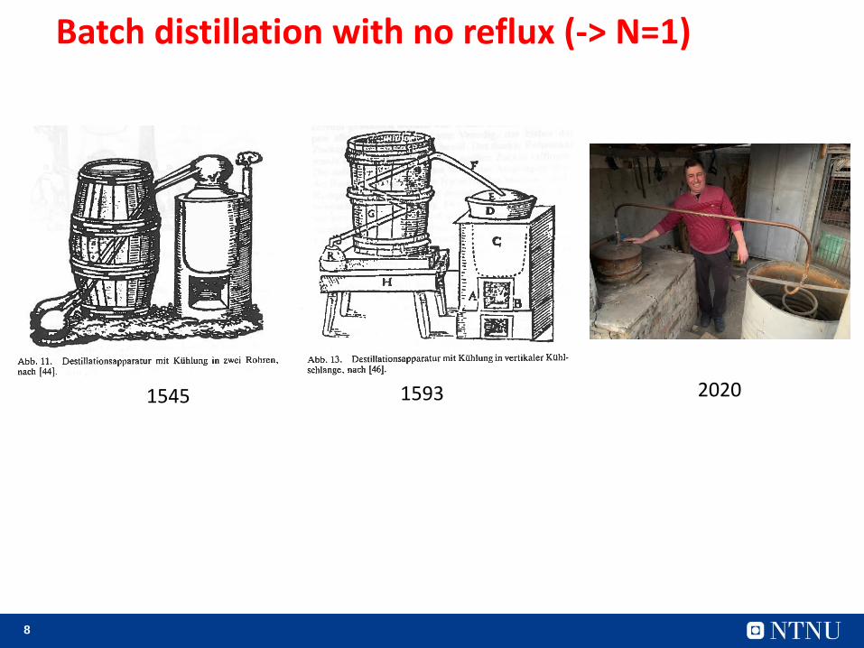
1545 1593

Batch distillation with no reflux (-> N=1)

2020

9

Continuous distillation with reflux (L)

V

L

stage 1

10

When use distillation?

• Liquid mixtures with difference in boiling point

• Unbeatable for high-purity separations• Essentially same energy usage independent of purity!

• Number of stages increases only as log of impurity!Fenske: Nmin = ln S / ln α

• Well suited for scale-up» Columns with diameters over 15 m

• Examples of unlikely uses of distillation: » High-purity silicon for computers (via SiCl3 distillation)

» Water – heavy-water separation (boiling point difference only 1.4oC)

Close-boiling mixture (α close to 1)• Need a lot of energy (heat) • and many stages

11

«Distillation is an inefficient process»

• This is a myth!

• By itself, distillation is an efficient process

– Typically, thermodynamic efficiency >50%

• It’s the heat integration that may be

inefficient.

– Yes, it can use a lot of energy (Qr=heat), but it

provides ~ the same energy as cooling (Qc) at

a lower temperature

12

• Separation into pure components

• Plot is for liquid feed, binary mixture

Thermodynamic efficiency of distillation

𝛼 = 10 𝛼 = 1

z = fraction light component in feed

𝜂

α = relative volatility

,

( ln (1 ) ln(1 ))

1( ) ln

1

id

s

s tot

W z z z z

Wz

− + − −= =

+−

Plot from I.J. Halvorsen.Ref: S. Skogestad, Chemical and Energy process engineering, CRC Press, 2009, pp. 224Ref: C.J. King, Separation processes, McGraw-Hill, 1971, 1980

13

2. Simple to model. Equilibrium stage concept

VLE: “Relative volatility model”Usually most important!• Activity coefficient (e.g. UNIFAC)• Or: Equation of state (e.g. SRK, PR)

Mi

VLE = Vapor-Liquid Equlibrium

Francis weir formula:

14

2. Simple to model. Equilibrium stage concept

VLE: “Relative volatility model”Usually most important!• Activity coefficient (e.g. UNIFAC)• Or: Equation of state (e.g. SRK, PR)

Mi

Modelling. Adjusting parameters1. VLE. May need experimental data2. Stages (N)

• Use steady-state model• Match steady-state compositions and temperature profiles

• Adjust N to get theoretical stages in each section (also for packed column)• Tray column: Can use Murphee efficiency. I use bypass on V and/or L

3. Holdup Mi. Match with dynamic data for compositions• Typical column holdup, ML = ΣMi

Tray column: 10% of column volumePacked column: 5% of column volume

4. Liquid dynamics: Make step in L and see how long it takes for change to reach bottom

• Francis weir formula: θL ≈ (2/3) ML / L

15

3. Dynamics

Example . Propylene-propane (C3-splitter, column D)

Mtot

F=σiMi

F= 111min

N = 110 theoretical stages

ΔTB=5.6K

= 1.12 (relative volatility at 15 bar)

Purities: 99.5% propylene (top) and 90% propane (bottom)

Assume constant molar flows

L/D = 19, D/F = 0.614

16

External flow change

Propylene-propane. Simulated composition response.

Increase reflux 0.4% (L = +0.05, D=-0.05) with V constant:

0 200 400 600 800 1000 1200 1400 1600 1800 20000.9945

0.995

0.9955

0.996

0.9965

0.997

0.9975

0.998

0 200 400 600 800 1000 1200 1400 1600 1800 20000.08

0.1

0.12

0.14

0.16

0.18

0.2

0 200 400 600 800 1000 1200 1400 1600 1800 20000.64

0.65

0.66

0.67

0.68

0.69

0.7

0.71

0.72

XD

0 1 2 3 4 5 6 7 8 9 100.0999

0.1

0.1001

0.1002

0.1003

0.1004

0.1005

0.1006

XB

2000 min

Xfeed stage

6 min

L

V

17

0 200 400 600 800 1000 1200 1400 1600 1800 20000

0.1

0.2

0.3

0.4

0.5

0.6

0.7

0.8

0.9

1

Increase in L +0.05

feed stage

18

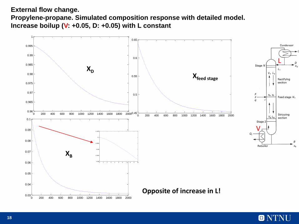
External flow change.

Propylene-propane. Simulated composition response with detailed model.

Increase boilup (V: +0.05, D: +0.05) with L constant

0 200 400 600 800 1000 1200 1400 1600 1800 20000.45

0.5

0.55

0.6

0.65

0 200 400 600 800 1000 1200 1400 1600 1800 20000.03

0.04

0.05

0.06

0.07

0.08

0.09

0.1

0 1 2 3 4 5 6 7 8 9 100.098

0.0985

0.099

0.0995

0.1

0.1005

0 200 400 600 800 1000 1200 1400 1600 1800 20000.96

0.965

0.97

0.975

0.98

0.985

0.99

0.995

1

Opposite of increase in L!

Xfeed stage

XB

XD

V

L

19

• What happens if we increase both L and V

at the same time?

• Then D and B are constant

• Internal flow change

V

L

20

Internal flow change.

Propylene-propane. Simulated composition response with detailed model.

Increase both L and V by same amount ( V = L = +0.05)

0 200 400 600 800 1000 1200 1400 1600 1800 20000

0.1

0.2

0.3

0.4

0.5

0.6

0.7

0.8

0.9

1

Very small effect

feed stage

22

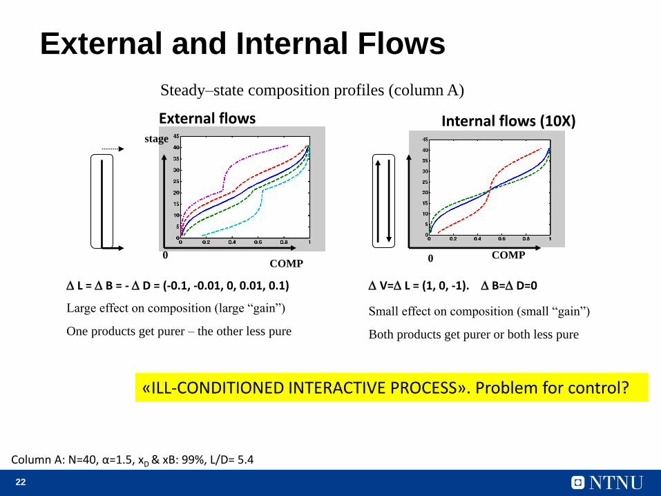
External and Internal Flows

Large effect on composition (large “gain”)

One products get purer – the other less pure

Small effect on composition (small “gain”)

Both products get purer or both less pure

Steady–state composition profiles (column A)

COMPCOMP

0 0

stage

External flows Internal flows (10X)

L = B = - D = (-0.1, -0.01, 0, 0.01, 0.1) V= L = (1, 0, -1). B= D=0

Column A: N=40, α=1.5, xD & xB: 99%, L/D= 5.4

«ILL-CONDITIONED INTERACTIVE PROCESS». Problem for control?

23

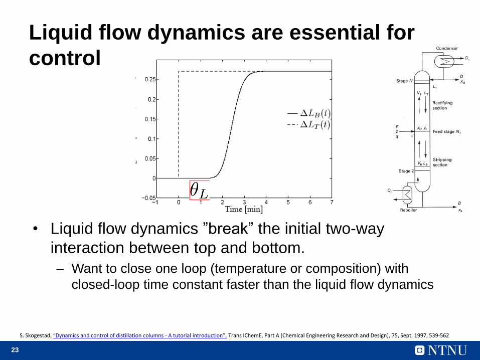
Liquid flow dynamics are essential for

control

• Liquid flow dynamics ”break” the initial two-way

interaction between top and bottom.

– Want to close one loop (temperature or composition) with

closed-loop time constant faster than the liquid flow dynamics

S. Skogestad, “Dynamics and control of distillation columns - A tutorial introduction”, Trans IChemE, Part A (Chemical Engineering Research and Design), 75, Sept. 1997, 539-562

24

Nonlinearity

Lii

Hi

X =lnx

x

Use logarithmic compositions

btm ii

i top

T -TX ln

T -T»

S. Skogestad, ``Dynamics and Control of Distillation Columns - A Critical Survey‘’, IFAC-symposium DYCORD+'92, Maryland, Apr. 27-29, 1992. Reprinted in Modeling, Identification and Control, Vol. 18, 177-217, 1997.

S. Skogestad, “Dynamics and control of distillation columns - A tutorial introduction”, Trans IChemE, Part A (Chemical Engineering Research and Design), 75, Sept. 1997, 539-562

With logarithmic compositions

26

Conclusion dynamics

• Dominant first order response – often close to integrating

from a control point of view

• Liquid flow dynamics decouples the top and bottom on a

short time scale, and make control easier

• Logarithmic transformations linearize the response

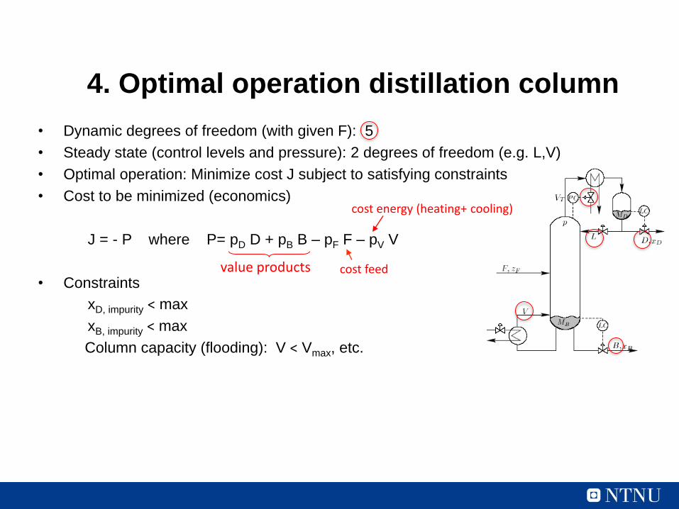
4. Optimal operation distillation column

• Dynamic degrees of freedom (with given F): 5

• Steady state (control levels and pressure): 2 degrees of freedom (e.g. L,V)

• Optimal operation: Minimize cost J subject to satisfying constraints

• Cost to be minimized (economics)

J = - P where P= pD D + pB B – pF F – pV V

• Constraints

xD, impurity < max

xB, impurity < max

Column capacity (flooding): V < Vmax, etc.

value products

cost energy (heating+ cooling)

cost feed

28

Expected active constraints distillation

• Valueable product: Purity spec. always active– Avoid product “give-away”

(“Sell water as methanol”)

– Saves energy

• Control implications: 1. Control valueable product at spec.

• Control D at 0.5% water

2. Overpurify other end to reduce loss

• Control B with methanol < 2%

• Overpurifying may not cost much energy (V) if enough stages

• If “few” stages: May be optimal to operate at max energy (V) to minimize loss of valuable product

valuable productmethanol

+ max. 0.5% water

cheap product(byproduct)water + max. 2%methanol

methanol+ water

29

5. Control

S. Skogestad, “The dos and don'ts of distillation columns control”,Chemical Engineering Research and Design (Trans IChemE, Part A), 85 (A1), 13-23 (2007).

30

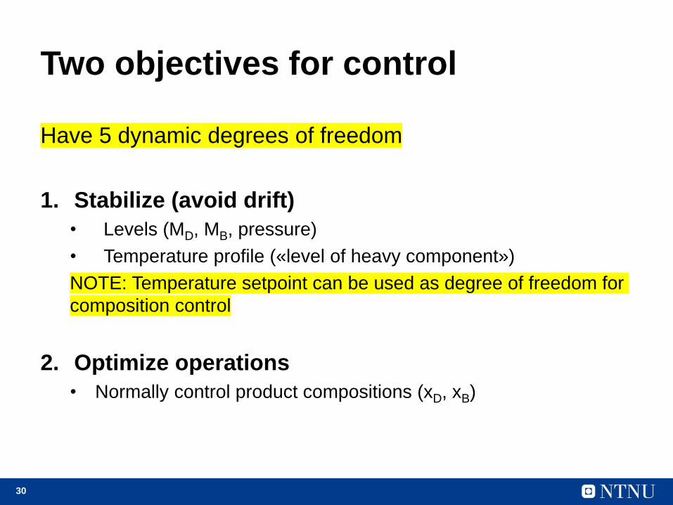
Two objectives for control

Have 5 dynamic degrees of freedom

1. Stabilize (avoid drift)

• Levels (MD, MB, pressure)

• Temperature profile («level of heavy component»)

NOTE: Temperature setpoint can be used as degree of freedom for

composition control

2. Optimize operations

• Normally control product compositions (xD, xB)

31

Issues distillation control

• The “configuration” problem

(pairings for level and pressure)

– Which are the two remaining

degrees of freedom?

• e.g. LV-, DV-, DB- and L/D V/B-

configurations

• The temperature control problem

– Which temperature (if any) should

be controlled?

• Composition control problem

– Control two, one or no

compositions?

TCTs TC

L

V

32

Stabilize temperature profile (“level of

heavy component”)

LIGHT

HEAVY

F

D

B

TC

• Temperature sensor should be located at «sensitive» stage (with high gain)• Typically in middle of top or bottom section

33

Which stage? Binary column

slope closely correlated with steady state gain

STAGE

TEMPERATURE PROFILE

34

Multicomponent column

Slope NOT correlated with steady-state gain

TEMPERATURE PROFILE

Conclusion: Temperature slope alone OK only for binary columns

35

Which configuration?

Level control top: Use L or D?

Seems almost impossible to control level with D (small range because need D>0)

LC

D (small)L (large)

VT (large)

FORTUNATELY: 1. Tight level control is NOT important2. Fast inner temperature loop gives indirect level control!

Conclusion: Recommend using D (and B) for level control!!Gives LV-configuration

However, for large L/D (>5):

Would like to use D because L is most effective for composition control

36

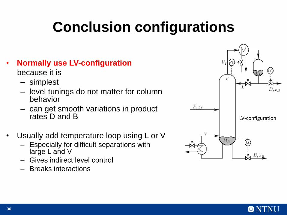
Conclusion configurations

• Normally use LV-configuration

because it is

– simplest

– level tunings do not matter for column behavior

– can get smooth variations in product rates D and B

• Usually add temperature loop using L or V– Especially for difficult separations with

large L and V

– Gives indirect level control

– Breaks interactions

LV-configuration

37

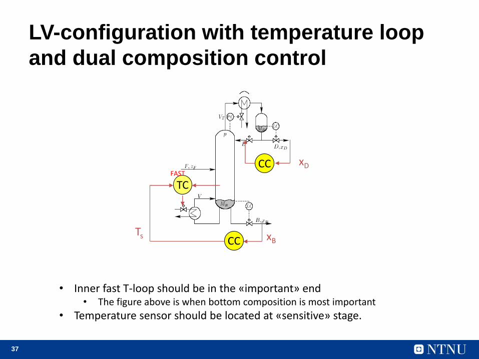
LV-configuration with temperature loop

and dual composition control

CC

LV

TC

Ts xB

CC xD

• Inner fast T-loop should be in the «important» end • The figure above is when bottom composition is most important

• Temperature sensor should be located at «sensitive» stage.

FAST

38

Myth of slow control

• Let us get rid of it!!!

Compare manual (“perfect operator”) and automatic control for column A:

• 40 stages,

• Binary mixture with 99% purity both ends,

• relative volatility = 1.5

• L/D = 5.4

– First “one-point” control: Control of top composition only

– Then “two-point” control: Control of both compositions

S. Skogestad, “Dynamics and control of distillation columns - A tutorial introduction”, Trans IChemE, Part A (Chemical Engineering Research and Design), 75, Sept. 1997, 539-562

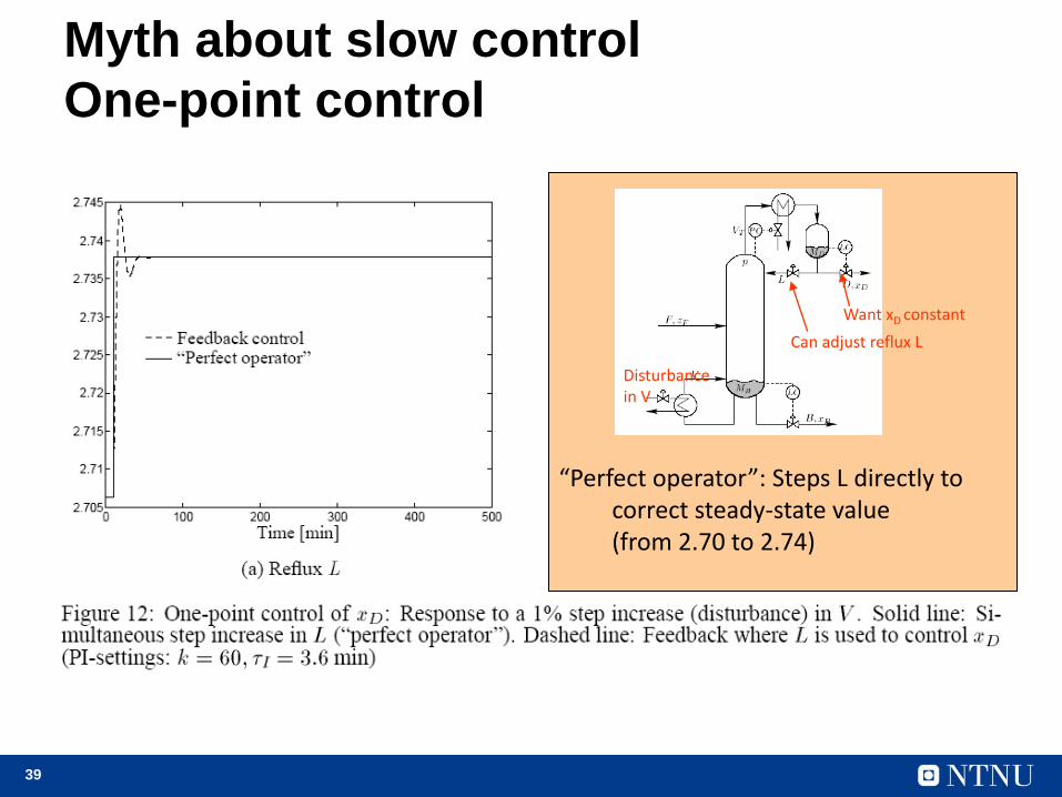
39

“Perfect operator”: Steps L directly to correct steady-state value (from 2.70 to 2.74)

Disturbance in V

Want xD constant

Can adjust reflux L

Myth about slow control

One-point control

40

“Perfect operator”: Steps L directlyFeedback control: Simple PI controlWhich response is best?

Disturbance in V

CC xDS

Myth about slow control

One-point control

41

Myth about slow control

One-point control

42

Myth about slow control

Two-point control

“Perfect operator”: Steps L and V directly Feedback control: 2 PI controllersWhich response is best?

CC xDS: step up

CC xBS: constant

V

L

43

Myth about slow control

Two-point control

V

L

44

Myth about slow control

Conclusion:

• Experience operator: Fast control impossible

– “takes hours or days before the columns settles”

• BUT, with feedback control the response can be fast!

– Feedback changes the dynamics (eigenvalues)

– Requires continuous “active” control

• Most columns have a single slow mode (without control)

– Sufficient to close a single loop (typical on temperature) to

change the dynamics for the entire column

45

Advanced control

May also add feedforward control from F (ratio V/F in this case)

Constraint on pressure drop, DPTop product valueable, xD

Overpurify bottom

xBmin: ConstraintxB*:Optimal xB (overpurify)

TCT

DPmax

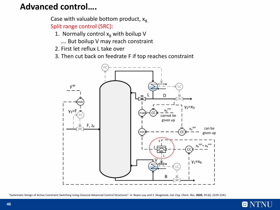
46

Case with valuable bottom product, xB.

Split range control (SRC):1. Normally control xB with boilup V

…. But boilup V may reach constraint2. First let reflux L take over 3. Then cut back on feedrate F if top reaches constraint

"Systematic Design of Active Constraint Switching Using Classical Advanced Control Structures". A. Reyes-Lua and S. Skogestad, Ind. Eng. Chem. Res. 2020, 59 (6), 2229-2241.

Advanced control….

47

Conclusion distillation control

• Not as difficult as often claimed

• LV-configurations recommended for most columns

• Use log transformations to reduce nonlinearity

• Use composition estimators based on temperature

• Usually: Close temperature loop (P-control OK)

• May use MPC if strong interactions between loops

CC

LV

Two-pointLV-configurationwith inner T-loop

TC

Ts

xB

CCxD

S. Skogestad, “The dos and don'ts of distillation columns control”,Chemical Engineering Research and Design (Trans IChemE, Part A), 85 (A1), 13-23 (2007).

48

Conclusion

1. Distillation as a separation process• In spite of claims to the contrary it's an efficient process

- it's the heat integration that may be inefficient

• Unbeatable for high-purity separations

2. Modelling • In principle it's simple

• Normally use equilibrium stage model

• The thermodynamics (VLE) are the most important

3. Dynamics• There is one dominant slow (drifting) mode

• related to the holdup of light and heavy key components inside the column

4. Optimal operation • Minimize energy usage (V) and maximize recovery of valuable component (J = pF F – pD D – pB B + pV V)

• subject to satisfying purity specifications

• Always active constraint: Purity of valueable product («avoid give-away»)

5. Control• Fist: stabilize the column (levels, pressure and one temperature)

• The temperature loop will speed up the slow mode, break interactions and provide indirect level control

• Next: Control active constraints and keep operation close to optimal

• May use MPC, but can usually do OK with advanced single-loop control

https://folk.ntnu.no/skoge/distillation/