26
Distinctive Image Features from Scale-Invariant Keypoints David G. Lowe – IJCV 2004 Brien Flewelling CPSC 643 Presentation 1
| Date post: | 22-Dec-2015 |
| Category: |
Documents |
| View: | 238 times |
| Download: | 0 times |

Distinctive Image Featuresfrom Scale-Invariant KeypointsDavid G. Lowe – IJCV 2004
Brien Flewelling
CPSC 643 Presentation 1

Overview Introduction
Motivation for this work
Related Work Corners and other Local Features Invariant descriptors Similar Detection, Different Descriptor

Overview Scalar Invariant Feature Transform
Scale Space Extrema Detection Keypoint Localization Orientation Assignment Keypoint Descriptor
Experiments and Tests Affine Changes, Large Data Bases, Object
Recognition Conclusions and Future Work
Motivation …. Why SIFT anyway? Highly Distinctive Features – Good Matching Detailed Descriptor – High Uniqueness Invariance to :
Scale – Zoom/Resampling In plane Rotation
Partial Invariance to : Lighting Change Out of plane Rotation

Related Work - Corner Detectors
Moravec (1981) – Stereo Matching using Corners
Harris and Stevens (1988) – Repeatability Improvements
Harris Corner Detector (1992) – commonly used in Structure from motion Solutions
“Large Gradients at a pre-determined scale”

Related Work - Feature Matching
Zhang and Torr (1995) – Use of correlation, least squares and geometric constraints to match Harris corners over large image ranges and motions.
Schmidt and Mohr (1997) – Use of a rotationally invariant feature descriptor for matching images in large databases with Harris corners.
Lowe (1999) – Extension of feature descriptors to achieve scale invariance.

Related Work – Stability to Changes Crowley and Parker (1984) – Scale Space Peaks and
matching of Tree Structures.
Lindberg (1993-94) – Scale Selection for good feature detection performance.
(Baumberg, 2000; Tuytelaars and Van Gool, 2000; Mikolajczyk and Schmid, 2002; Schaffalitzky and Zisserman, 2002; Brown and Lowe, 2002).
– Affine Covariant Features

Related Work – Other Features Nelson and Selinger (1998) – Image Contours
Matas et al., (2002) – Maximally Stable Extremal Regions
Carneiro and Jepson (2002) – Phase Based Local Features
Schiele and Crowley (2000) – Multidimensional Histogram Descriptors

SIFT – Scale Space Extrema Detection Scale Space – A 1-parameter function of the
image data Gaussian Scale Space - Convolution with a
Gaussian Kernel … No False Structure! L(x, y, σ ) = G(x, y, σ) I(x, y)∗ G(x, y, σ ) = (1/2πσ2)*exp(-(x2+y2)/(2σ2))
Detection of ExtremaD(x, y, σ ) = (G(x, y, kσ) − G(x, y, σ)) I(x, y)∗ = L(x, y, kσ) − L(x, y, σ ).

The Difference of Gaussian Space For constant scaling of σ this approximates the
Laplacian of Gaussian
Approximating the derivative of the Gaussian function with respect to sigma we can obtain

SIFT – Scale Space Extrema Detection Construct the DOG scale
space K – factor of separation S – number of S+3 images in the stack for
each octave Resample and repeat
For each location compare to its 26 nearest neighbors in scale space retain only minima and maxima

SIFT – Local Extrema Detection Sampling of scale space is a balance between
density of samples and the arbitrary feature frequencies
Test the reliability of matches over matching tasks vs. sampling frequencies
The most stable and useful frequencies can be detected with coarse sampling in scale.

SIFT – Local Extrema Detection Once a Scale Space
Extrema is localized: Calculate an
interpolated fit for location, scale and ratio of principle curvatures
Compute a local Taylor Series Expansion of the DOG function. Find the Zero crossing of the derivative of this function:

Evaluating Edge Responses by Comparing Principle Curvatures The DOG space will have a large response to edges.
Poorly defined extrema have strong principle curvature along the edge but a weak principle curvature normal to it.
We may examine the relationship between principle curvatures by looking at the eigenvalues of the approximated Hessian matrix.

The Hessian Matrix and Keypoint Rejection
The Hessian Matrix is approximated using Neighbor Differences
The ratio of the square of the trace to the determinant has a special relationship to the eigenvalue ratio

SIFT – Orientation Assignment To achieve rotational invariance, the local
gradient orientations are examined to define a principle direction.
A magnitude weighted orientation histogram is calculated using the DOG image of nearest scale.

SIFT – Keypoint Descriptor The keypoint descriptor structures the local
image information in the DOG image of nearest scale with respect to the assigned orientation.
Inspired by work by Edelman, Intrator, and Poggio (1997), the feature descriptor lists the gradient orientations in a structured vector

SIFT – Keypoint Descriptor The number of elements in the descriptor vector is calculated by the product of
the number of histogram bins and the number of orientation directions typically 4x4x8 = 128

Experiments – Affine Change The SIFT descriptor was
tested against a database of 40,000 keypoints.
The percent repeatability of correct matches vs. affine performs better than 50% for up to 50 degree rotations out of plane

Experiments - Large Databases
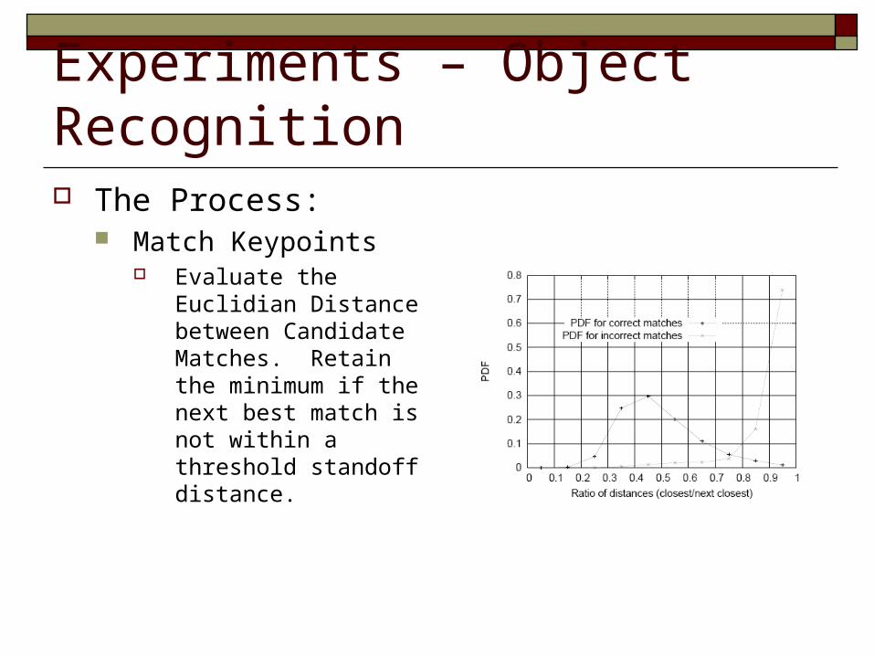
Experiments – Object Recognition The Process:
Match Keypoints Evaluate the Euclidian
Distance between Candidate Matches. Retain the minimum if the next best match is not within a threshold standoff distance.
Experiments – Object Recognition When searching for the best match a
prioritized Best Bin First search is used. For purposes of object recognition a Hough
Transform is used to cluster objects in pose space
Large Error Bounds, does not account well for affine variations – 4 DOF vs. 6 DOF
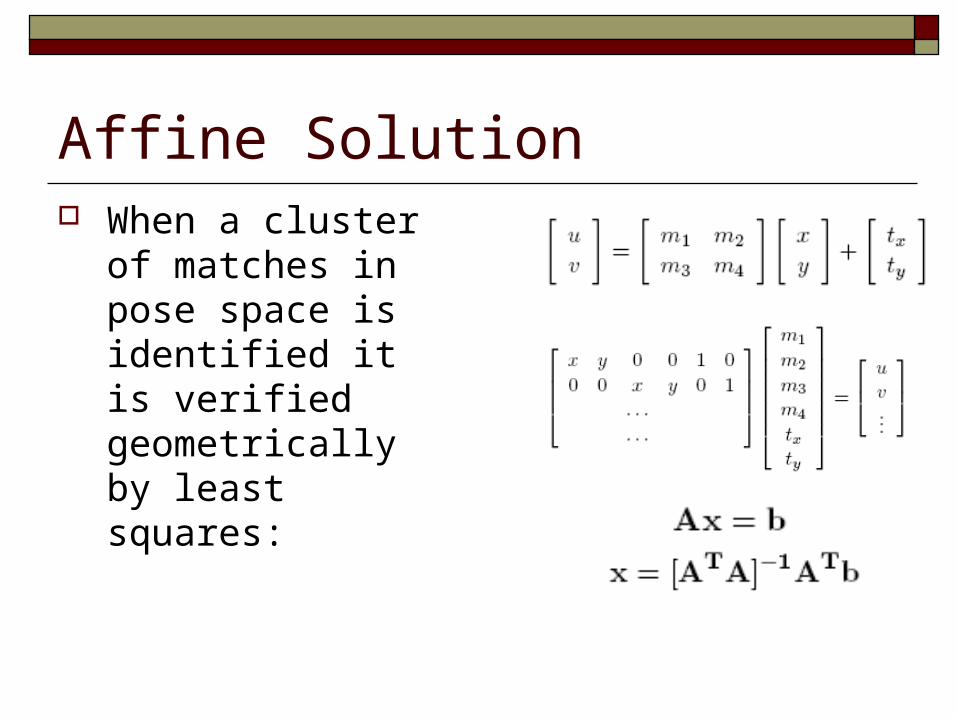
Affine Solution When a cluster of
matches in pose space is identified it is verified geometrically by least squares:

Results

Conclusions The SIFT algorithm has strength in its
detailed descriptor and makes it robust to many transformations
Matching performs with reasonable repeatability for high clutter, occlusion, changes in scale, rotation, and illumination
This method works well for object recognition and the analysis of planar patches but struggles with 3d object geometry

Future Work Color SIFT
Object Classes base on SIFT Feature Distributions
SIFT based High Dynamic Range imagery Project to come stay tuned


