DISTORTION ESTIMATES FOR PLANAR DIFFEOMORPHISMS

DISTORTION ESTIMATES FOR PLANAR DIFFEOMORPHISMS

SHELDON NEWHOUSE

Dedicated to Yasha Pesin on the occasion of his sixtieth birthday.

ABSTRACT. We define new distortion quantities for diffeomorphisms of the Eu-clidean plane and study their properties. In particular, we obtain composition rulesfor these quantities analogous to standard rules for maps of an interval. Our resultsapply to maps with unbounded derivatives and have important applications in thetheory of SRB measures for surface diffeomorphisms.

CONTENTS

0. Introduction. 21. Dilation and Distortion in One Dimensional Systems 42. Statement of Results 53. Proof of Proposition 2.1 274. Proofs of Propositions 2.2 and 2.3 295. Proof of Theorem 2.4 316. Proof of Theorem 2.5 356.1. Some simple matrix estimates 356.2. Some linear estimates for hyperbolicity 376.3. Distortion for Markov compositions of maps whose Jacobian matrices

are diagonal at a point 396.4. Distortion for compositions of hyperbolic and parabolic maps 457. Proofs of Theorems 2.6, 2.7, and 2.8 797.1. Proof of Theorem 2.6 797.2. Proof of Theorem 2.7 807.3. Proof of Theorem 2.8 87References 878. Glossary 89Index of Special Symbols and Notations 89

Date: July 6, 2007.1

2 SHELDON NEWHOUSE

0. INTRODUCTION.

Consider a smooth self map f : M→M of a smooth manifold M. One of the mainproblems in the theory of dynamical systems is to describe the asymptotic behaviorof the orbits x, f (x), f 2(x), . . . for various points x ∈ M. Specific objects of impor-tance include the estimation of the Hausdorff dimension of various invariant sets,the calculation of topological and measure-theoretic entropies, and the quantitativeunderstanding of the evolution of sets of positive Lebesgue measure. In this lattercase, one often is interested in the existence and properties of so-called natural orSRB measures. A fundamental tool in the study of all of these concepts is the in-vestigation of quantitative objects associated to the orbits of submanifolds γ whichare expanded from time to time under iteration by the map f . One of the main suchquantitative objects is the volume ratio. One seeks to control the ratio

vol( f n(E))vol( f n(F))

of the Riemannian volumes of sets E ⊂ γ, F ⊂ γ as n increases. The questionreduces to the estimation of the volume dilation ratios

(1)Jγ f n(z)Jγ f n(w)

for z,w∈ γ where Jγ f n(z) denotes the infinitesimal volume expansion of f n alongγ at z.

It should be noted that various second derivative estimates related to (1) are typ-ically called distortion estimates in the literature. We will be more precise on ourversion of these notions later in the sequel.

Techniques for estimating (1) when γ is an unstable manifold of a point in a uni-formly hyperbolic set and the derivatives of f are bounded are well-known and goback to Sinai [12] (see also Lectures 16 and 17 in [13] for more general systems).In one dimensional dynamics, the quantities (1) even go back to Denjoy who usedthem in his solution of the Poincare problem of topological transitivity of C2 diffeo-morphisms of the circle with irrational rotation numbers. More recently, they playa central role in the study of absolutely continuous invariant measures as in [2], [4],and [7], .

In two dimensional dynamics, one often encounters a piece of unstable manifoldof a fixed point (or a nearby curve) whose forward iterates exhibit a combinationof expansion, contraction, and folding. The control of the quantities (1) in thesesituations becomes complicated. A major part of the work of Benedicks-Carleson[1], Mora-Viana [8], Wang-Young [14], etc., on the study of strange attractors andSRB measures for Henon-like maps involves the control of these dilation ratios.

DISTORTION ESTIMATES FOR PLANAR DIFFEOMORPHISMS 3

There are basically two methods currently available to estimate dilation ratiosalong iterates of curves. We refer to these, respectively, as the critical point methodand the induced map method

(1) Critical point method. This involves the identification of a set called thecritical set C such that the images of relevant curves fold as they first passnear C. Away from C one has hyperbolic behavior. The control of distortionis obtained by an iterate by iterate analysis along orbits. The orbit is brokeninto pieces which exhibit hyperbolic behavior while they stay at some dis-tance from C, and which which exhibit folding when they approach C. Oneuses more or less standard estimates along the hyperbolic pieces, and onedoes a careful analysis of how the orbits behave near the folds. Basically,one puts these last orbits in positions so that long stretches of hyperboliciterates undo the damage to expansion contributed by the folds. The secondorder derivatives of each iterate involved are uniformly bounded. In one-dimensional dynamics, the critical set C is simply the set of critical points ofthe map (i.e., where the first derivative vanishes). The very definition of theanalogous critical set in two dimensional dynamics (in consideration of or-bits of infinite length) was a major breakthrough of Benedicks and Carlesonin [1]. It is at the heart of the works of Benedicks-Carleson, Mora-Viana,Wang-Young, etc., mentioned above.

(2) Induced Map Method This involves taking high iterates of the original map,so that one can more or less always consider compositions of hyperbolicmaps. The effects of folds are absorbed by taking maps h each of whichcan be expressed as compositions h = F ◦ f or h = F ◦ f ◦G where F =f n and G = f m are iterates of the original map f . In these compositions,the folding occurs at the points where f is applied, and the maps F and Gare uniformly hyperbolic. The resulting maps h again become uniformlyhyperbolic, but with unbounded derivatives and bounded distortion. Theprocess continues to higher and higher iterates of the original map f via aninduction in which the maps F and G are successively replaced by the newmaps h and the construction is repeated. The detailed construction involvesa careful analysis of the relationship between the maps F,G and the areaswhere the folds given by f occur. The technique of controlling distortion formaps with unbounded derivatives was first considered by Jakobson in [4] inproving the existence of a positive measure set of parameters r such thatthe logistic map fr(x) = rx(1− x) has an absolutely continuous invariantmeasure.

The purpose of the present paper is to develop tools for the Induced Map Methodin two dimensional systems. The main application of these tools is to aid in proving

4 SHELDON NEWHOUSE

the existence of so-called chaotic attractors and associated SRB measures for suchdiffeomorphisms. As a related new consequence of some of the results presentedhere we mention that one can obtain stronger versions of the results in [6]. In thelatter paper, we considered maps fi defined on closed full-height subrectangles Eiof a given rectangle with certain expansion and bounded distortion properties. Weused the Whitney Extension Theorem to extend each map fi to a neighborhood Uiof Ei with related expansion and bounded distortion properties. The results givenhere allow one to avoid the use of the Whitney Extension Theorem and get thesame results of [6] by assuming the expansion and bounded distortion propertieshold only on the interiors of the rectangles Ei.

We also mention that, in connection with work on bifurcation theory [11], J.Palis and J-C. Yoccoz have also obtained estimates for dilation ratios for surfacediffeomorphisms with unbounded derivatives (see [10]) which are similar in spiritto those given here, but which use very different techniques from ours and requiredifferent assumptions. A significant way in which their assumptions differ fromours is that the hyperbolic maps they consider have images whose diameters areuniformly bounded below. This assumption, which is sufficient for their applica-tions to bifurcation theory, is, at least in our present understanding, too strong to beapplicable to Henon-like maps.

In concluding this introduction, we remark that it is evident that some parts ofthe present paper are rather technical and involve many different symbols. As anaid to the reader, we have appended a glossary which gives the page numbers fordefinitions of most of the symbols used in the paper.

Acknowlegement. This work grew out of on-going joint work with M. Jakobsonon Henon-like maps. We have developed various approaches to two-dimensionaldistortion estimates which are similar in spirit but differ in technical details. Theapproaches extend the techniques of distortion estimates developed in [5] and [6].The present work presents one of these approaches. It is a pleasure to acknowledgemany useful conversations with Michael Jakobson in connection with this work.

1. DILATION AND DISTORTION IN ONE DIMENSIONAL SYSTEMS

Our main results concern two dimensional diffeomorphisms. However, as moti-vation for these results, it seems worthwhile to begin with some related concepts inone-dimensional systems.

Let f be a C2 diffeomorphism from a closed real interval E to its image. Onedefines the dilation ratio drt( f ) = drt( f ,E) of the pair ( f ,E) to be the quantity

drt( f ,E) = supz,w∈E

| D f (z) || D f (w) |

.


One next defines the distortion Θ( f ,E) of the pair ( f ,E) by

Θ( f ,E) = supz∈E

| D2 f (z) || D f (z) |

| E |

where D f (z),D2 f (z) are the first and second derivatives of f at z and | E | is thelength of E.

The following relation between the dilation ratio and the distortion is well-knownand follows easily from the Mean Value Theorem.

If J ⊆ E is a subinterval, thenDilation Ratio Formula for One Dimensional Distortion:

(2) drt( f ,J)≤ exp(

Θ( f ,E)| J || E |

).

A second well-known and useful inequality relates the distortion of a compositionh = f ◦g of interval maps to the distortions of the factor maps f , g (see [2]) or [4]).

Composition Formula for One Dimensional Distortion:Suppose f , g are C2 diffeomorphisms defined on intervals E f ,Eg, respectively,

and g(Eg)⊇ E f . Let Eh = g−1(E f ) and h = f ◦g.Then, writing Θ(h) = Θ(h,Eh), Θ( f ) = Θ( f ,E f ), and Θ(g) = Θ(g,Eg), we have

(3) Θ(h)≤Θ( f )exp(

Θ(g)| Eh || Eg |

)+Θ(g)

| Eh || Eg |

.

Formula (3) can be used to show (e.g. as in [6] and [4]) that if f1, f2, . . . is asequence of expanding diffeomorphisms such that Θ( fi)≤K for all i and the lengthsof the images of fi are bounded below, then there is a constant K1 such that for everyn≥ 1, we have

Θ( f1 ◦ . . .◦ fn)≤ K1.

This, in turn, can be used to establish the existence of absolutely continuousinvariant measures (see [2], [4]).

Now, we proceed to two dimensional analogs of the above distortion concepts.

2. STATEMENT OF RESULTS

Throughout this section we denote by R2 the Euclidean plane. We let <,> be itsstandard inner product and, unless otherwise stated, norms will be with respect tothis inner product.

Our first results give analogs of estimates (2) and (3) along smooth curves for adiffeomorphism f : R2 → R2.

6 SHELDON NEWHOUSE

Let E be a subset of R2. By a diffeomorphism f : E → E ′ we mean a C2 diffeo-morphism f defined on an open neighborhood of E such that E ′ = f (E).

We use the terminology that a standard rectangle in R2 is the product I× J oftwo real intervals.

A parametrized rectangle is a triple (φ, I × J,E) in which I × J is a standardrectangle, E is a subset of the plane, and φ is a C2 diffeomorphism from I× J ontoE. We will frequently suppress the objects φ, I× J in the parametrized rectangle(φ, I× J,E) and simply call the set E a rectangle.

Letting (x,y) denote coordinates in R2, and let (φ, I× J,E) be a parametrizedrectangle in R2. A full-width curve γ in I×J is a C2 curve γ(t) = (x(t),y(t)), definedfor t ∈ I, such that the map t → x(t) is a diffeomorphism from I onto I. Similarly,a full-height curve γ in I× J is a C2 curve γ(t) = (x(t),y(t)), defined for t ∈ J, suchthat the map t → y(t) is a diffeomorphism from J onto J.

Two parametrized rectangles (φ, I× J,E),(φ1, I1× J1,E1) are compatible if I1 =I,J1 = J,E1 = E) and the diffeomorphism φ ◦ φ

−11 from I× J to itself carries full-

height curves to full-height curves and full-width curves to full-width curves.A full-width subrectangle of (φ, I× J,E) is a triple (ψ1, I× J1,E1) where J1 is

a subinterval of J, and there is a rectangle (ψ, I× J,E) which is compatible with(φ, I×J,E) such that ψ1 is the restriction of ψ to I×J1. We also sometimes simplysay that E1 is a full-width subrectangle of E. Similar definitions and considerationsapply to full-height subrectangles.

Let E be a rectangle and f : E → E ′ be an C2 diffeomorphism from E to its imageE ′.

Given a C2 curve γ = γ(t),a ≤ t ≤ b with non-vanishing tangent vectors, whoseimage lies in E, let

γ(t) =dγ

dtand

γ(t) =γ(t)| γ(t) |

denote, respectively, the tangent and unit tangent vectors to γ at γ(t).For z = γ(t) in γ, let

Jγ f (z) = | D fγ(t)(γ(t)) |be the Jacobian of f along γ at z.We also use the notation z = γ(t), z = γ(t) when z = γ(t) is a point in the curve γ.Let ds(γ) denote the arclength element on γ, and let curv(γ(t)) denote the curva-

ture of γ at γ(t). Set curv(γ) = supt curv(γ(t)). Denote the arclength of γ by | γ |.Define


Ψ1(z, f ,γ) =| D fz || D fz(z) |

,

and

Ψ2(z, f ,γ) =| D2 f (z)(z,z) || D f (z)(z) |

| γ |,

Ψ1( f ,γ) = supz∈γ

Ψ1(z, f ,γ),

Ψ2( f ,γ) = supz∈γ

Ψ2(z, f ,γ).

Our first result is an analog of (2) for two dimensional systems.

Proposition 2.1. (Two dimensional dilation ratio estimate) Under the above no-tation, if z,w ∈ γ, then we have

(4)Jγ f (z)Jγ f (w)

≤ exp[(Ψ2( f ,γ)+Ψ1( f ,γ)curv(γ)| γ |)

dγ(z,w)| γ |

]Remark. If we introduce the quantity

Ψ( f ,γ) = Ψ2( f ,γ)+Ψ1( f ,γ)curv(γ)| γ |,

then we can rewrite (4) in a form which is analogous to the one dimensionaldilation ratio expression:

(5)Jγ f (z)Jγ f (w)

≤ exp(

Ψ( f ,γ)dγ(z,w)| γ |

).

The quantity Ψ2( f ,γ) is reminiscent of the one-dimensional distortion, but wesee that the ratio Ψ1( f ,γ) of the derivative norms and the curvature of γ enter in tothe formula. In keeping with the analogy with one dimensional systems, we definethe distortion of f along the curve γ to be the quantity Ψ( f ,γ). Note that if γ is aline segment, then Ψ2( f ,γ) = Ψ( f ,γ) since curv(γ) = 0.

Next, we wish to consider analogs of the composition formula (3) for two dimen-sional maps. The proper concept involves properties of the mappings on curves.

Let f : E f → E ′f , g : Eg → E ′g be C2 diffeomorphisms of rectangles onto theirimages. We say that g Markov precedes f , written f � g or g ≺ f , if E ′g

TE f

is a full-width subrectangle of E f and g−1(E ′gT

E f ) is a full-height subrectangle

8 SHELDON NEWHOUSE

of Eg. In that case the map h = f ◦ g is a C2 diffeomorphism from the rectangleEh = g−1(E ′g

TE f ) onto its image E ′h. We call h a Markov composition of f and g.

Proposition 2.2. (Distortion formula for two dimensional Markov composi-tions). Suppose that h = f ◦ g is a Markov composition of f and g and that γgis a full-width curve in Eg such that γ f = g(γg)

TE f is a full-width curve in E f . Let

γh = γgT

Eh. Then,

(6) Ψ2(h,γh)≤Ψ2( f ,γ f )exp

(Ψ(g,γg)

| γh || γg |

)+Ψ1( f ,γ f )Ψ2(g,γg)

| γh || γg |

.

Now, we obtain an upper bound for the quantity Ψ1( f ,γ) if the mapping f satis-fies certain cone conditions.

Let 0 < α be a fixed real number. The standard α−cones Kuα, Ks

α in R2 aredefined to be

(7) Kuα = {v = (v1,v2) : | v2 | ≤ α| v1 |},

(8) Ksα = {v = (v1,v2) : | v1 | ≤ α| v2 |}.

A cone in R2 is the image of Ku1 by a linear isomorphism P. For a subset E ⊂R2

and mapping φ : E → Gl(2,R), the function z → Kz = φ(z)(Ku1 ) will be called a

cone field in E. If φ is continuous we speak of a continuous cone field in E. Wesometimes use the notation K for the cone field z→Kz.

If K is a cone field in E and f : E → E ′ is a C1 diffeomorphism, we have thepush-forward cone field f?K on E ′ defined by

f?(K ) f z = D fz(Kz).Similarly, if K ′ is a cone field in E ′, we have the pull-back cone field f ?K ′ in E

defined by

f ?(K ′)z = D f−1f z (K ′

f z).

These operations obviously extend to pairs of cone fields (K1,K2) by f?(K1,K2)=( f?(K1), f?(K2), f ?(K1,K2) = ( f ?(K1), f ?(K2).

Given cone fields K 1, K 2, we say that K 1 ⊆K 2 if we have K 1z ⊆K 2

z for all z.Let C = (C u,C s) be a pair of cone fields on E. We say that C is a disjoint pair of

cone fields if C uz

TC s

z = {(0,0)} for z ∈ E.Given two linearly independent vectors, v,w ∈ R2, we define the angle between

them, ang(v,w), by


(9) ang(v,w) = arccos(

< v,w >

| v || w |

)Given the disjoint pair of cone fields C = (C u,C s) on E, we define

ang(z,C u,C s) = inf{| ang(v,w) | : v ∈ C uz \{0},w ∈ C s

z \{0}}and

ang(C ) = inf{ang(z,C u,C s) : z ∈ E}We call ang(C ), the angle of the cone field pair C .If ang(C ) > 0 on E we call the cone field pair C separated on E. Of course, if C

is a continuous disjoint cone field pair on E and E is compact, then C is separatedon E. In the continuous case, it is clear that

(10) 0 < ang(C ) <π

2.

In this paper we will only consider separated cone field pairs, so, by convention,when we say cone field pair we always mean separated cone field pair.

Let E be a subset of R2, let f : E → E ′ be a diffeomorphism, and let C be aseparated cone field pair on E

SE ′, with C = (C u,C s). We call f a C −map if

f?(C u) ⊂ C u and f ?(C s) ⊂ C s (on their appropriate domains of course). A curveγ : t → γ(t) in E is a C u−curve if d

dt γ(t)∈C uγ(t) for all t. Similarly, define C s−curves.

For a C−map f : E → E ′ and z ∈ E, let

muz = inf

v∈C uz \{0}

| D fz(v) || v |

,

msz = inf

v∈C sf z\{0}

| D f−1f z (v) || v |

.

Thus, muz is the least expansion of D fz on vectors in C u

z \ {0} and an analogousstatement holds for ms

z.Also, define

mC = infz∈E

ms(z)mu(z).

We call mC the domination coefficient of the cone pair C (or of the pair ( f ,C )).We say that f expands the cone field C u on E if

10 SHELDON NEWHOUSE

infv∈C u

z \{0},z∈E

| D fz(v) || v |

> 1.

We also say that f | C u is expanding.We call f : E →E ′ hyperbolic if there is a continuous pair of separated cone fields

C = (C u,C s) on ES

E ′ such that(1) f is a C -map.(2) f expands C u and f−1 expands C s.

When we wish to emphasize the cone field pair C in this definition, we will saythat f is C−hyperbolic.

In several cases below the specific rates of expansion of a C− hyperbolic mapwill be important for us. Accordingly, we set

Ru = infz∈E

muz , Rs = inf

z∈Ems

z, R = (Ru,Rs),

and

Rmin = min(Ru,Rs) > 1.

When we wish to include the pair R = (Ru,Rs) in the definition of hyperbolicity,we will say that f is (R,C )−hyperbolic, (R,C u,C s)−hyperbolic, or (Ru,Rs,C u,C s)-hyperbolic.

Remark. The concepts we have defined above work naturally with respect tocompositions. We have the following.

(1) Suppose g : E → E ′ and f : E ′→ E ′′ are C−maps where C is a separatedcone field pair on E

SE ′

SE ′′. Then, f ◦g is also a C -map.

(2) Suppose g : E → E ′ and f : E ′→ E ′′ are (R,C )−hyperbolic maps, then sois f ◦g.

Our next proposition gives a convenient estimate of Ψ1( f ,γ) for C−maps.

Proposition 2.3. Assume that f is a C−map with domination coefficient mC . Letβ = sin(ang(C )) where ang(C ) is the minimum angle of the cone field pair C =(C u,C s), and let γ be a C u−curve.

Then,

(11) Ψ1( f ,γ)≤ 2(1+mC )β

2mC.

Let 0 < α < 1. For simplicity, if Kα = (Kuα,Ks

α) is the standard α− cone fieldpair, and f is (R,Kα)−hyperbolic, we say that f is (R,α)−hyperbolic. We will


also use a pointwise version. We say that f is (R,α,z)−hyperbolic if D f (z) mapsKu

α into itself, is an Ru−expansion on Kuα, D f−1( f (z)) maps Ks

α into itself, and isan Rs−expansion on Ks

α.Our next result states roughly that an arbitrary composition of Markov related

(R,α) hyperbolic maps, each with bounded distortion along full-width Kuα−curves,

again has bounded distortion.

Theorem 2.4. Let Q be a standard rectangle, n ≥ 2 be a positive integer, and letE1,E2, . . .En be a sequence of full-height subrectangles of Q. For 0 < α < 1, Rmin >1, and 1 ≤ i < n, let fi : Ei → E ′i be an (R,α) hyperbolic map such that fi Markovprecedes fi+1 and E ′i ⊂ Q. Let z1 ∈ E1 and let γ1 be a full-width (C2) Ku

α−curvein E1 containing z1, and let curv(γ1) be its maximum curvature. Let Fi = fi ◦ fi−1 ◦. . . ◦ f1, zi+1 = Fi(z1), and let γi+1 be the connected component of Fi(γ1)

TEi+1

containing zi+1. For 2≤ i≤ n, let

ηi = F−1i−1(γi).

Assume there is a constant K0 > 0 such that

(12) sup1≤i≤n

Ψ2( fi,γi) < K0.

Then, there a constant K = K(K0,R,curv(γ1), | γ1 |) > 0 such that

(13) Ψ(Fn−1,ηn)≤ K.

Remark.(1) Corollary 3.4 in the paper of Palis and Yoccoz [10] contains a similar result

under stronger assumptions for both fi and f−1i when γ1 is a line segment.

(2) The result does not require that the rectangles be closed. Thus one can applytogether with Proposition 2.1 it to prove Proposition 8.1 in [6], allowing oneimprove the results of [6] as we indicated earlier.

Next, we move to the case of compositions of hyperbolic and parabolic maps.It will be convenient to consider analogs of the distortion like quantity Ψ2 above

using affine coordinates in which certain maps have diagonal Jacobian matrices.Such coordinates are sometimes called adapted coordinates.

Let z ∈ R2,v,w be two linearly independent vectors in R2, and let v = v| v | , w =

w| w | be the associated unit vectors.

Let e1 =(

10

)e2 =

(01

)be the standard basis vectors of R2. Let Az,v,w be

the affine automorphism of R2 such that

12 SHELDON NEWHOUSE

(1) Az,v,w(z) = z(2) DAz,v,w(v) = e1(3) DAz,v,w(w) = e2

Given linearly independent vectors v,w, let

v? = D fz(v),w? = D f−1f z (w)

Set

(14) f = fz,v,w = A f z,v?,w ◦ f ◦A−1z,v,w?

Given an embedded C1 curve γ = {γ(t),a ≤ t ≤ b}, let | γ | denote its arclength,and, for z1,z2 ∈ γ, let dγ(z1,z2) denote the arclength of the subarc of γ from z1 to z2.

Now, assume that f : E → E ′ is C -hyperbolic with a separated cone field pairC = (C u,C s) defined on E

SE ′.

A C2 curve γ = γ(t) is a C u−curve if γ(t) ∈ E and γ(t) ∈ C uγ(t) for all t.

Let z = γ(t) for some t, let z = γ(t), and let w be a non-zero vector in C sf z. Set

γz,w = Az,z,w?(γ). Recall that curv(γ) denotes the maximum of the curvatures of thecurve γ at its various points.

Define

Θ(z, f ,w,γ) = max(i, j)

| D2 fz,z,w(z)(ei,e j) || D fz,z,w(z)(e1) |

| γz,w |

and

Θ2(z, f ,w,γ) = max(i, j)6=(1,1)

| D2 fz,z,w(z)(ei,e j) || D fz,z,w(z)(e1) |

| γz,w |

Θ(z, f ,γ) = supw∈C s

f z

Θ(z, f ,w,γ)

Θ( f ,γ) = supz∈γ

Θ(z, f ,γ)

Θ2(z, f ,γ) = supw∈C s

f z

Θ2(z, f ,w,γ)

Θ2( f ,γ) = supz∈γ

Θ2(z, f ,γ)


We call Θ( f ,γ) the Θ−distortion of f along γ, and we call Θ2( f ,γ) the Θ2−distortionof f along γ. When γ is understood, we refer simply to the Θ−distortion or Θ2−distortionof f .

Observe that if Kuα ⊂ C u

z and Ksα ⊂ C s

z , and γ is a horizontal line segment, then

(15) Ψ2(g,γ)≤ KΘ( f ,γ)

for some constant K depending on α.Let I = [a,b], J = [c,d] be two closed real intervals.Given a curvilinear rectangle φ : I×J → E, we define the vertical curves to be the

curves φ({x}× J) for x ∈ I, and the horizontal curves to be the curves φ(I×{y})for y ∈ J. The vertical boundary of E is the set consisting of the pair of curves{a}× J,{b}× J, and the horizontal boundary is the set consistimg of the curvesI×{c}, I×{d}.

When the context makes it clear, we identify the parameterized rectangle with itsimage and refer to the vertical and horizontal boundaries of E.

An admissible rectangle is a curvilinear rectangle whose horizontal boundarycurves are horizontal line segments and whose vertical boundary curves are Ks

α−curves.If E is an admissible rectangle, and z ∈ E, the full-width horizontal line segment

through z in E is called the E−horizontal line segment through z, and any of theseis called an E−horizontal line segment.

An image-admissible rectangle is the image E ′ = f (E) where E is an admissi-ble rectangle and f is an (R,α)-hyperbolic map. A horizontal curve in an image-admissible rectangle E ′ = f (E) is the f−image of a full-width horizontal line seg-ment in E. For z ∈ E, we denote the horizontal curve through z by `h(z).

We now consider parabolic maps.Let W be an admissible rectangle, and K > 0. Let f be a C2 diffeomorphism and

γ be a C2 curve in the domain of f . We say f maps γ K−parabolically into W if(1) both endpoints of γ are mapped into the same vertical boundary curve γb of

W ,(2) For any non-zero vector v tangent to γ, | D f (v) | ≥ | v |(3) At any point z of f (γ) where the slope of the tangent vector is greater than

or equal to 1, the curvature of f (γ) at z is greater than or equal to K(4) the curvature of γb at any of its points is less than K

2 .Observe that, it follows from these definitions that there is a unique point z′c(γ) ∈

f (γ) at which the tangent vector to f (γ) is parallel to some tangent vector to γb.Let E,W be rectangles, and assume that W is admissible and E is image-admissible.Given a C2 plane curve γ(t) = (x1(t),x2(t)), t ∈ [a,b], with first and second

derivatives γ′(t) = (x′1(t),x′2(t)),γ

′′(t) = (x1(t),x2(t)), we define the C1 size of γ

to be

14 SHELDON NEWHOUSE

| γ |C1 = maxt∈[a,b],i=1,2

(| xi(t) |, | x′i(t) |),

Similarly, we define the C2 size of γ to be

| γ |C2 = maxt∈[a,b],i=1,2

(| xi(t) |, | x′i(t) |, | x′′i (t) |).

Given two curves γ0(t),γ1(t), t ∈ [a,b] we define the C1 and C2 distances, respec-tively, between them to be

d1(γ0,γ1) = | γ0− γ1 |C1,

and

d2(γ0,γ1) = | γ0− γ1 |C2.

The arclength of the curve γ is denoted | γ |.Let K > 0, we say f maps E K−parabolically into W if f maps each horizontal

curve in E K−parabolically into W .When the domain E of f and the constant K are understood, we sometimes simply

say the the map f is parabolic.Next, we consider certain compositions h = f ◦ p ◦ g where f ,g are hyperbolic

maps and p is a parabolic map.Let f : E f → E ′f , g : Eg → E ′g be (R,α)−hyperbolic, with E f and Eg admissible

rectangles. Let W be another admissible rectangle containing E f as a full-heightsubrectangle, and suppose that p : E ′g →W is a C2 diffeomorphism from E ′g into W .We say

(16) f � p� g

if(1) p(E ′g) = (p◦g)(Eg)

TE f consists of two connected components Z1, Z2 each

of which is a full-width subrectangle of E f(2) the rectangles (p◦g)−1(Zi) have full-height in Eg for i = 1,2, and(3) E ′f contains at least one full-height vertical line segment

Assuming that f � p� g, let Eh,i = (p◦g)−1Zi for i = 1,2. The rectangle Eh,i isa full-height subrectangle of Eg. Let

(17) hi denote the restriction of f ◦ p◦g to Eh,i.


��

��

Eh,2Eh,1

Z1

−1p f(E )

Eg E’g

��

��

p ( )E’g

Ef

E’f

Z2

W

fg

p

FIGURE 1. The maps f , p,g

We will be interested in conditions guaranteeing that the map hi is also (R,α)−hyperbolic,and we will obtain certain distortion estimates of hi on horizontal line segments inEh,i in terms of distortion estimates of g and f and geometric properties of f , p,g.

Figure 1 shows the geometric structure of the maps f , p,g.Given a rectangle E, let lw(E) be the largest full-height subrectangle of E such

that each point w ∈ lw(E) contains a full-height vertical line segment in E. Ingeneral, lw(E) may not exist, but if E is image-admissible, and its top and bottomboundaries are close to each other compared to their lengths, then lw(E) does exist.

For each point w ∈ E ′f , we define the principal vertical line segment, `v(w), as-sociated to w to be the full-height vertical line segment in lw(E ′f ) which is closestto w. Thus, if w ∈ lw(E ′f ), then `v(w) is simply the full-height vertical line segmentthrough w. Otherwise, it is the vertical boundary curve of lw(E ′f ) which is closestto w.

For w ∈ E ′f with w = f (z), let `−1v (z) = f−1(`v(w)). This is the principal vertical

curve of z. It is a Ksα full-height curve in E f . For any curve γ in E f , and z ∈ γ such

that γT

`−1v (z) 6= /0, define the vertical curve distance of (z,γ) to be

vcd(z,γ) = distγ(z, `−1v (z)),

where distγ(z, `−1v (z)) is the arclength of the shortest subarc of γ joining z to

γT

`−1v (z)).

16 SHELDON NEWHOUSE

Define the maximum vertical curve distance of γ to be

(18) vcd(γ) = supz∈γ

vcd(z,γ).

Notice that if each point of E ′f is contained in a full-height vertical line segmentin E ′f , then, vcd(γ) = 0.

Define the quantity w f (z,γ) to be the infimum of the lengths of E f−horizontalline segments which meet γ. That is, if L(γ) is this collection of horizontal linesegments, set

(19) w f (z,γ) = inf`∈L(γ)

| ` |.

For a curve γ, let mincurv(γ) denote the minimum of the curvatures of γ at any ofits points, and recall that curv(γ) denotes the maximum of the curvatures of γ at anyof its points. We call

vcurv(E f ) = maxz∈E f

curv(`−1v (z))

the vertical curvature of E f .For a point z = z1 ∈ Zi with associated points z0 = (p◦g)−1z,z2 = f (z), we have

the cone fields C u(z) = D(p ◦ g)(Kuα(z0)),C s(z) = D f−1(z2)(Ks

α(z2)). Define theminimum angle

(20) ang def= in fz∈Ziang(C u(z),C s(z)).

We remark that the assumptions of Theorem 2.5 below will imply that ang > 0.In the setting of Theorem 2.5, f , p,g will be maps such that f � p� g, γg will be

a full-width horizontal line segment in Eg, z0 will be a point in γg, z1 will be g(z0),and z2 ∈ E f will be p(z1). The map h will be one of the hi defined in (17), the curveγ f will be the E f−horizontal line segment passing through z2, and the curve γh willbe the corresponding line segment γg

TEh,i = (p◦g)−1((p◦g)(γg)

TZi).

Letting a ∼ b mean that ab is bounded above and below, it will turn out that, for

the curve γ = (p◦g)(γh), we have

vcd(γ)∼ dist(z1, `−1v (z1))

ang.

For notational brevity below, we write


(21) Θ( f ) = Θ(z2, f ,γ f ), Θ(h) = Θ(z0,h,γh), Θ(g) = Θ(z0,g,γg),

and

(22) Θ2( f ) = Θ2(z2, f ,γ f ), Θ2(h) = Θ2(z0,h,γh), Θ2(g) = Θ2(z0,g,γg),

For a line segment γ in Eg, we set

(23) J?(g,γ) = supz∈γ

| det(Dg(z)) |Jγg(z)2

and

J1(g,γ) =J?(g,γ)

ang.

We let ∂le f t(E f ),∂right(E f ) denote, respectively, the left and right vertical bound-ary curves of E f .

Let γ be a curve both of whose boundary points lie in the same component of thevertical boundary of the rectangle E f , and let ∂γ(E f ) denote this vertical boundarycomponent. Define the critical distance from γ to E f to be

cdist(γ,E f ) = maxz∈γ

dist(z,∂γ(E f ).

For a map f , and a point z, set

(24) J f = J f (z) = | det(D f (z)) |.In formulas (25)–(52) below, the quantities J f and f1x are to be evaluated at

appropriate points z ∈ γ f , and the quantities Jg and g1x(z) are to be evaluated atappropriate points z ∈ γg. All of the inequalities are assumed to be uniform in thosepoints z.

Recall from (19) and (18) that, for z ∈ E f and γ a curve through z, the quantityw f (z,γ) is the smallest width of horizontal line segments meeting γ, and vcd(z,γ) isthe smallest distance along γ to the pull-back of the closest vertical curve in E ′f tof (z).

Theorem 2.5. (Composition formula for distortion of hyperbolic and parabolicmaps)

Let 0 < α < 13 , 1 < Rmin, K0 > 0 be constants. Using the above notation, assume

that f : E f → E ′f , g : Eg → E ′g are (R,α)−hyperbolic, p : Ep →W is a C2 embed-ding, and that f � p� g. Fix i = 1 or i = 2. Let h be the mapping hi defined in (17)

18 SHELDON NEWHOUSE

above with corresponding rectangle Zi, and let Eh = Eh,i = (p◦g)−1(Zi). Let z0 be apoint in Eh, let γg be the Eg−horizontal line segment through z0, and let γh = γg

TEh.

Let z1 = g(z0) ∈ E ′g, z2 = p(z1) ∈ E f , and let γ f be the E f−horizontal line segmentin E f through z2. Let ρh(z2) = vcd(z2,(p ◦ g)(γh)), w f (z2) = w f (z2,(p ◦ g)(γh)),and let the various Θ,Θ2 quantities be defined as in (21) and (22) above.

Then, there are positive constants K1,C0 > 1 and 0 < ε0 < 1 depending on K0,α,the C2 size of p, and the C1 size of p−1, with the following properties.

Suppose that p maps g(γg) K0−parabolically into W, and, in addition,

(25)J f

| f1x |2<

19,

(26) | γ f | ≤ K0 cdist((p◦g)(γg),E f ),

(27) max(1,Θ(g))| γ f |

2

ang5 < K0,

(28)ρh(z2)w f (z2)

max(1,Θ( f )) < ε0 ang

(29) vcurv(E f ) < ε0 min(1,mincurv((p◦g)(γg)),

and

(30) Rmin ·ang > C0.

Then, h is also (R,α)−hyperbolic.Moreover, setting

(31) ν0 =Θ2( f )ang2 +

Θ(g)| γ f |2

ang5 +| γ f |ang2 +

Θ(g)ang

| γh || γg |

,

(32) ν1 = ν0 + J1( f ,γ f ),

and


ν2 =(

Θ2( f )ang2 +

| γ f |ang2

)J1(g,γh)exp

(Θ(g)ang

| γh || γg |

)

+Θ(g)J1(g,γh)

ang| γh || γg |

+Θ2(g)ang

| γh || γg |

(33)

we have

(34) Θ(h)≤Θ( f )exp(K1ν1)+K1ν0

and

(35) Θ2(h)≤ K1ν2.

20 SHELDON NEWHOUSE

Remark. The expressions (31)–(35) above involve many terms and are com-plicated. With a view toward eventual applications, we wish to simplify these es-timates. This will involve addtitional assumptions which, together with the cor-responding theorems, we describe next. Our principle goal is to give conditionsunder which compositions of many hyperbolic and parabolic maps have uniformlybounded distortion. This is the content of Theorem 2.8 below which may be re-garded as one of the main results of this paper.

Consider a composition h = f ◦ p◦g with f ,g, p,γg,γh,γ f as in Theorem 2.5. Notethat this is actually an abuse of notation. The domain of the composition f ◦ p ◦ gis a union of two full-height subrectangles Eh,1 and Eh,2 of the domain Eg of g. Wecontinue to use h to denote the restriction of f ◦ p◦g to one of the rectangles Eh,i.

Set Sg = g(γg).In the following the numbers δi will all be suitably small positive constants.Assumptions (A):

(36)J f

| f1x |2≤| γ f |ang

,

and, there are constants δ1,δ2,δ3 in (0,1), K2 > 1 such that

(37) ang < 1, | Sg |< 1,| γ f |ang2 < K2| Sg |−δ2 | γh |

| γg |< 1,

(38) Θ(g) < K2| Sg |1−δ1,

(39) K2| Sg |> ang≥ K−12 | Sg |1+δ2,

and

(40) 4K32 | Sg |−δ1−2δ2

(| γh || γg |

)δ3

< 1.

Then, we have the following estimate for Θ(h):

Theorem 2.6. Let K1 be as in Theorem 2.5, and let δ3 be as in (40). In addition tothe hypotheses (25)–(30) of Theorem 2.5, suppose that assumptions (A) are satisfied,and set


ν3 =Θ2( f )ang2 +

(| γh || γg |

)1−δ3

.

Then, we have

(41) Θ(h)≤Θ( f )exp(K1ν3)+K1ν3.

To obtain a simplified estimate for Θ2(h), we make some more assumptions.Let L1 > 0 and L2 > 0 be such that

(42) Θ(g)≤ L1, exp

(Θ(g)ang

| γh || γg |

)≤ L2.

Set

(43) K3 = max(1,K1L1,K1L2,K2).

Assumptions (B):

(44) K(1−δ3)(1+2δ2)2 | Sg |(1−δ3)δ2 < 1,

(45) K33

Jg

ang3| g1x |2<

14,

(46)K3| γg |

1−δ3

ang

(| γh || γg |

)δ3

<14,

(47) Θ2( f ) < | γ f |1−δ3,

(48) Θ2(g) < | γg |1−δ3,

and

(49)K3

3 Jg

ang2| g1x |2

(1

| γ f |

)1−δ3

<14.

Assumptions (C):

22 SHELDON NEWHOUSE

The map h = f ◦ p◦g satisfies

(50)Jg

ang2+δ4| g1x |1+δ3<

13K3

,

(51)Jg

ang3| g1x || γh |

δ3 <1

3K3,

and

(52)1

ang

(| γh || γg |

)δ3

<1

3K3.

We make some further definitions.We call the map h = f ◦ p◦g a basic central composition map (or bcc map) if it

satisfies the hypotheses (16), (25)–(30) of Theorem 2.5, and Assumptions (A) and(B).

Observe that, for simplicity of notation, we continue to consider h as the restric-tion of the actual composition f ◦ p ◦ g to one of the connected components of itsdomain. A similar remark holds for all of the maps h,H,H j, f ,g we consider below.The domain of each such map is a single rectangle.

Consider a sequence g j, 0 ≤ j ≤ k of (R,α)−hyperbolic maps such that each

H jdef= g j−1 ◦ p◦g j is a bcc map.

Let h0 = g0 and, for 1≤ j ≤ k, let

h j = g0 ◦ p◦g1 ◦ . . .◦ p◦g j,

and assume that

h j−1 � p� g j.

For each j, let Eg j ,Eh j denote, respectively, the domains of the maps g j,h j. Theseare admissible rectangles.

Given a point zk in Ehk , let zk−1 = p◦gk(zk), zk−2 = p◦gk−1(zk−1), . . . , z0 ∈ Eg0 .Thus, each z j ∈ Eh j ⊂ Eg j .Let γg j

denote the full-width line segment in Eg j which contains z j, and let γh j=

γg j

TEh j . Let ang j denote the minimum angle as in (20) obtained by substituting

h j−1 for f and g j for g.The sequence

T (zk,hk) = ((γgk, γhk

,angk), (γgk−1, γhk−1

,angk−1), . . . , (γg1, γh1

,ang1))


will be called the triple sequence of the pair (zk,hk). It is defined for each pointzk in the domain Ehk of a composition hk as above.

A central composition map (or cc map) is a composition

(53) hk = g0 ◦ p◦g1 ◦ p◦g2 · · · ◦ p◦gk.

as above such that, for each point zk ∈ Ehk the triple sequence T (zk,hk) satisfies

(54)| γh j−1

|ang2

j< K2| Sg j |

−δ2| γh j

|| γg j

|< 1

for each 1≤ j ≤ k.We call the map hk the concatenation of the maps H j, for 1≤ j≤ k, and we write

H = hk = H1�H2 . . .�Hk.Note that the maps g j may themselves be concatenations of bcc maps. However,

since each map H j is (R,α)−hyperbolic and Rmin > 1, there is a maximal numberof bcc maps whose concatenation gives hk.

We define the rank of the cc map H to be this maximal number of bcc mapswhose concatenation gives H. It may be larger than k.

The cc map H is called an enhanced cc map or ecc map if H can be written as acomposition H = f ◦ p◦g in which f and g are cc maps and assumptions (16), (A),(B) and (C) are satisfied.

We now get the following simplified estimates for Θ2(h).

Theorem 2.7. Suppose that h = f ◦ p ◦ g is a bcc map or a cc map of rank k ≥ 2where f is a cc map of rank k−1 satisfying the above conditions. Then,

(55) Θ2(h)≤

(| γh || γg |

)1−δ3

.

If, in addition, h is an ecc map, then we have

(56) Θ2(h)≤ | γh |1−δ3.

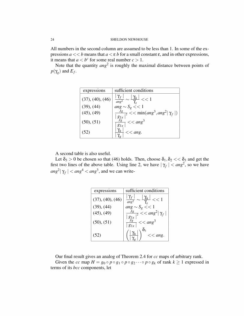
Remark. It is natural to ask when the expressions in assumptions (A), (B), and(C) are satisfied in applications. While the geometric meaning of some of theseexpressions is clear, others may be somewhat more opaque. Also, there often arefurther relations between these quantities in typical applications. To help make theexpressions involved more intuitive, we give two tables below which informally de-scribe some situations which guarantee that some of the expressions above occur.

24 SHELDON NEWHOUSE

All numbers in the second column are assumed to be less than 1. In some of the ex-pressions a << b means that a < ε b for a small constant ε, and in other expressions,it means that a < bc for some real number c > 1.

Note that the quantity ang2 is roughly the maximal distance between points ofp(γg) and E f .

expressions sufficient conditions

(37), (40), (46)| γ f |ang2 ∼

| γh |γg

<< 1

(39), (44) ang∼ Sg << 1(45), (49) Jg

| g1x |2<< min(ang3,ang2| γ f |)

(50), (51) Jg| g1x |

<< ang3

(52) | γh || γg |

<< ang.

A second table is also useful.Let δ3 > 0 be chosen so that (46) holds. Then, choose δ1,δ2 << δ3 and get the

first two lines of the above table. Using line 2, we have | γ f | < ang2, so we haveang2| γ f |< ang4 < ang3, and we can write-

expressions sufficient conditions

(37), (40), (46)| γ f |ang2 ∼

| γh |γg

<< 1

(39), (44) ang∼ Sg << 1(45), (49) Jg

| g1x |2<< ang2| γ f |

(50), (51) Jg| g1x |

<< ang3

(52)(| γh || γg |

)δ3

<< ang.

Our final result gives an analog of Theorem 2.4 for cc maps of arbitrary rank.Given the cc map H = g0 ◦ p ◦ g1 ◦ p ◦ g2 · · · ◦ p ◦ gk of rank k ≥ 1 expressed in

terms of its bcc components, let


h0 = g0

h1 = g0 ◦ p◦g1

h2 = h1 ◦ p◦g2

h3 = h2 ◦ p◦g3...

hk = hk−1 ◦ p◦gk.

For 0 ≤ i ≤ k, we call hi the the i− th left-segment of H. Of course, each hi is acc map itself.

Theorem 2.8. Let H = g0 ◦ p◦g1 ◦ p◦g2 · · · ◦ p◦gk be a cc map such that there isa constant K4 > 0 such that

(57) Θ(gi)≤ K4

for each 0 ≤ i ≤ k. Let zk be a point in Ehk with associated triple sequenceT (zk,hk). Let δ3 be as in Theorem 2.7, and let K1 be as in Theorem 2.6.

Assume further that

(58) max

Θ2(h0)ang2

1,

(| γh1

|| γg1

|

)1−δ3≤ K4

2K1,

and there is a constant 0 < ξ < 1 such that for each i ∈ [2,k],

(59)K1

ang2i

(| γhi−1

|| γgi−1

|

)1−δ3

+K1

(| γhi

|| γgi

|

)1−δ3

≤ K4ξi.

Then,

(60) Θ(H)≤

(K4

k

∑i=0

ξi

)exp

(K4

k

∑i=0

ξi

).

In particular, if

K5 =

(K4

∞

∑i=0

ξi

)exp

(K4

∞

∑i=0

ξi

),

then,

26 SHELDON NEWHOUSE

Θ(hk)≤ K5

for all k ≥ 1.

Remark. One way to interpret condition (59) is the following. As we add thecompositions p◦gi to hi−1 to form hi, the ratios

| γhi|

| gi |can decrease exponentially. Also, the angles angi can decrease exponentially.

However, the angi decrease slowly enough so that the quantity

| γhi−1|

ang2i | gi−1 |

still decreases exponentially.


3. PROOF OF PROPOSITION 2.1

Let I be the domain of the curve t → γ(t), and let t1, t2 ∈ I be such that γ(t1) =w,γ(t2) = z. Replacing γ by t → γ(−t) (and I by −I) if necessary, we may assumethat t1 ≤ t2.

Write z(t) for the unit vector in the direction of γ(t) and s = sγ(t) for the arclengthparameter. All equalities and inequalities in this proof will be up to multiplicationby possibly different constants K.

First, we have

| D fγ(t2)(z(t2)) || D fγ(t1)(z(t1))) |

= exp(Z t2

t1

ddt

log | D fγ(t)(z(t)) |dt)

≤ exp(Z t2

t1

∣∣∣∣ ddt

log | D fγ(t)(z(t)) |∣∣∣∣ dt)

.

Next, using standard estimates and the Cauchy-Schwarz inequality, we have

∣∣∣∣ ddt

log | D fγ(t)(z(t)) |∣∣∣∣ =

∣∣∣∣∣ 1| D fγ(t)(z(t)) |

ddt| D fγ(t)(z(t)) |

∣∣∣∣∣=

∣∣∣∣∣ 1| D fγ(t)(z(t)) |

< ddt D fγ(t)(z(t)),D fγ(t)(z(t)) >

| D fγ(t)(z(t)) |

∣∣∣∣∣≤

| ddt D fγ(t)(z(t)) || D fγ(t)(z(t)) |

≤| D2 fγ(t)(γ(t)),z(t)) |+ | D fγ(t)( d

dt z(t)) || D fγ(t)(z(t)) |

≤| D2 fγ(t)(z(t)),z(t)) || γ(t) |+ | D fγ(t) || d

dt z(t) || D fγ(t)(z(t)) |

≤| D2 fγ(t)(z(t)),z(t)) || γ(t) |

| D fγ(t)(z(t)) |+Ψ1( f ,γ)| d

dt z(t) |

Moreover,

∣∣∣∣ ddt

z(t)∣∣∣∣ =

∣∣∣∣ ddsγ

z(sγ(t))∣∣∣∣ · ∣∣∣∣dsγ

dt

∣∣∣∣= curv(γ(t)) · | γ(t) |.

28 SHELDON NEWHOUSE

Hence,

∣∣∣∣ ddt

log | D fγ(t)(z(t)) |∣∣∣∣ ≤

| D2 fγ(t)(z(t)),z(t)) || D fγ(t)(z(t)) |

| γ(t) |

+ Ψ1( f ,γ)curv(γ(t))| γ(t) |

=| D2 fγ(t)(z(t)),z(t)) || γ |

| D fγ(t)(z(t)) || γ(t) || γ |

+ Ψ1( f ,γ)curv(γ(t))| γ | | γ(t) || γ |

≤ (Ψ2( f ,γ)+Ψ1( f ,γ)curv(γ)| γ |) | γ(t) || γ |

which implies (4) and completes the proof of Proposition 2.1. QED


4. PROOFS OF PROPOSITIONS 2.2 AND 2.3

Proof of Proposition 2.2:Consider maps f ,g,h, etc. as in the statement of Proposition 2.2. For a point z in

a curve γ, let z denote the unit tangent vector to γ at z. So, consider z ∈ γh.We wish to estimate

| D2hz(z,z) || Dhz(z) |

| γh |

in terms of f ,g.Note that

gz =Dgz(z)| Dgz(z) |

,

and, the Mean Value Theorem gives us a point z1 ∈ γh such that

| Dgz1(z1) || γh |= | γ f |.We have

| D2hz(z,z) || Dhz(z) |

| γh | =| D2 fgz(Dgz(z),Dgz(z)) |+ | D fgz(D2gz(z,z)) |

| D fgz(Dgz(z)) || γh |

≤| D2 fgz(gz,gz) || γ f || Dgz(z) |

| D fgz(gz) || γh || γ f |

+| D fgz || (D2gz(z,z)) || D fgz(gz) || Dgz(z) |

| γh |

=| D2 fgz(gz,gz) || γ f || Dgz(z) |

| D fgz(gz) || Dgz1(z1) |+| D fgz || (D2gz(z,z)) || D fgz(gz) || Dgz(z) |

| γh |

≤ Ψ2( f ,γ f )exp

(Ψ(g,γg)

| γh || γg |

)+Ψ1( f ,γ f )Ψ2(g,γg)

| γh || γg |

Taking the supremum as z varies in γh gives (6), completing the proof of Propo-sition 2.2. QED.

Proof of Proposition 2.3 .Assume the notation of Proposition 2.3.Thus β = sin(ang(C u,C s)) and mC is the domination coefficient of C .Let z ∈ γ and v1,v2 be unit vectors in TzR2 with v2 ∈ C u

z tangent to γ. We willshow that

(61) | D fz(v1) | ≤2

β2

(1+mC

mC

)| D fz(v2) |.

30 SHELDON NEWHOUSE

Let w ∈ C sf z be a non-zero vector, and let

w1 =D f−1

f z (w)

| D f−1f z (w) |

Then, w1 is a unit vector in C sz and we have

(62) | D fz(w1) | ≤ (msz)−1 =

muz

mszmu

z≤ | D fz(v2) |

mszmu

z.

Let < w1,v2 >= η. Since C u, C s are disjoint cone fields, we have that | η |< 1.Writing v1 = α1v2 +α2w1, we have the equations

< v1,v2 > = α1 +α2η

< v1,w1 > = α1η+α2

and the inverse equations

(63)(

α1α2

)=

11−η2

(1 −η

−η 1

) (< v1,v2 >< v1,w1 >

)from which we get

(64) max(| α1 |, | α2 |) <2

1−η2

Thus,

| D fz(v1) | ≤ | α1 || D f (v2) |+ | α2 || D f (w1) |

≤ 21−η2 (1+

1ms

zmuz)| D f (v2) |

≤ 21− cos(ang(C u

z ,C sz ))2 (1+

1mC

)| D fz(v2) |

=2

β2

(1+

1mC

)| D fz(v2) |

=2

β2

(1+mC

mC

)| D fz(v2) |

as required for (61). QED.


5. PROOF OF THEOREM 2.4

We first need a lemma which we call the Exponential Increment Lemma. In thispaper we only need the special case of the lemma in which bn = cn for all n. Infuture applications, however, the lemma will be needed in a form with bn < cn.Since the proof is practially the same, we present this slightly more general formhere.

Lemma 5.1. (Exponential Increment Lemma). Let (ai),(bi),(ci), i ≥ 0, be threesequences of positive real numbers.

Assume that

(65) a0 ≤ b0exp(c0),

and

(66) n > 0 =⇒ an ≤ an−1 exp(cn)+bn.

Then, for each n≥ 0, we have

(67) an ≤

(n

∑i=0

bi

)exp

(n

∑i=0

ci

).

Proof.By induction on n.The inequality (67) is true for n = 0. Assume that it holds for n.Then,

an+1 ≤ an exp(cn+1)+bn+1

≤

(n

∑i=0

bi

)exp

(n

∑i=0

ci

)exp(cn+1)+bn+1

≤

(n

∑i=0

bi

)exp

(n+1

∑i=0

ci

)+bn+1

≤

(n

∑i=0

bi

)exp

(n+1

∑i=0

ci

)+bn+1

(exp

n+1

∑i=0

ci

)

≤

(n+1

∑i=0

bi

)exp

(n+1

∑i=0

ci

).

32 SHELDON NEWHOUSE

QED.In particular, if

(68)∞

∑i=0

bi < ∞,

and

(69)∞

∑i=0

ci < ∞,

then we have the following upper bound for the sequence (an),n≥ 0.

(70) an ≤

(∞

∑i=0

bi

)exp

(∞

∑i=0

ci

).

Moving to the proof of Theorem 2.4, we shall prove the following two separatestatements.

(1) There is a constant K2 > 0 such that,

(71) Ψ2(Fn−1,ηn)≤ K2

(2) There is a constant K3 > 0 such that, for each 1≤ i≤ n,

(72) curv(γi)≤ K3.

Once (71) and (72) are established, we proceed as follows.Since each fi is a (K u

α,K sα)−map. and the composition of (R,α)−hyperbolic

maps is again (R,α)−hyperbolic, we have that Fn−1 is a (K uα,K s

α)−map. Thus,using Proposition 2.3, we can find a constant C(α) > 0 such that

Ψ1(Fn−1,ηn)≤C(α).By definition, this gives

Ψ(Fn−1,ηn) = Ψ2(Fn−1,ηn)+Ψ1(Fn−1,ηn)curv(ηn)| ηn |≤ K2 +C(α)K3| Q |def= K

as required.Let us proceed to prove (71). We will apply Proposition 2.2 and Lemma 5.1.For each n ≥ 2, let h = Fn−1, γh = ηn, g = f1, γg = γ1, f = fn−1 ◦ fn−2 ◦ . . . ◦

f2,γ f = g(ηn).


Since f and g are (K uα,K s

α)−maps, we have

max(Ψ1(g,γg),Ψ1( f ,γ f ))≤C(α).Letting | Q | denote the width of Q, we have that | γi | ≤ | Q | for each i, so, with

K4 = K0 +C(α)curv(γg)| Q |, we have

Ψ(g,γg) = Ψ2(g,γg)+Ψ1(g,γg)curv(γg)| γg |≤ Ψ2(g,γg)+C(α)curv(γg)| Q |≤ K4.

Hence, using Proposition 2.2, we have

Ψ2(Fn−1,ηn) = Ψ2(h,γh)


(Ψ(g,γg)

| γh || γg |

)+C(α)Ψ2(g,γg)

| γh || γg |


(K4| γh || γg |

)+C(α)K0

| γh || γg |

.(73)

From the Mean Value Theorem, there is a point τn ∈ γh such that

(74) | γh |=| γn |

| JγhFn(τn) |

.

Since, Fn−1 is a composition of n−1 (R,Kuα,Ks

α)-hyperbolic maps, we have

1| Jγh

Fn−1(τn) |≤ R−n+1

u ,

giving

(75)| γh || γg |

=| γh || γ1 |

≤ R−n+1u | Q || γ1 |

−1.

Now, for n = 0,1,2, set

(76) bn = cn = max(K0,1) = a0 = a1,

and, for n≥ 3, set bn = C(α)K0R−n+1u | Q || γ1 |

−1 and cn = K4R−n+1u | Q || γ1 |

−1,and an−1 = Ψ2( fn−1 ◦ fn−2 . . .◦ f2).

Then, setting

34 SHELDON NEWHOUSE

K2 = (∞

∑i=0

bn)exp(∞

∑i=0

cn),

and using our definitions and (73), we may apply Lemma (5.1) to give

Ψ2(Fn−1,ηn)≤ K2

which is (71).Next, consider statement (72).This uses standard graph transform methods as in [3] except that our diffeomor-

phisms have unbounded derivatives. Since the image curves γi have their lengthsbounded below, the methods are entirely similar to those use in the proof of Theo-rem 6.1 in [6]. So we will not repeat them here.

We do note that similar methods will be used below in the proof of Lemma 6.9below, a case in which the lengths of the image curves may be short, and must beincluded in the estimate for the curvatures.

This completes the proof of Theorem 2.4. QED.


6. PROOF OF THEOREM 2.5

6.1. Some simple matrix estimates. We consider the standard matrix norm

| A |= sup| v |=1

| Av |.

First, we recall the following elementary estimate for the deformation of anglesunder linear isomorphisms.

Lemma 6.1. Let A be a 2×2 real matrix, and let u,v be two linearly independentunit vectors. Then,

(77) | sin(ang(Au,Av)) |= | detA || Au || Av |

| sin(ang(u,v)) |.

Proof.Using the standard cross product of planar vectors, we have

| u× v |= | sin(ang(u,v)) |and

| detA || u× v | = | Au×Av |= | Au || Av || sin(ang(Au,Av)) |.

Now, (77) follows immediately. QED.Next, we give some norm estimates of the matrix DAz,v,w.

Lemma 6.2. The following estimates involving the affine map Az,v,w are valid.

(78) | DAz,v,w | ≤√

2| sin(ang(v,w)) |

and

(79) | DA−1z,v,w | ≤

√2.

Proof.We first take the second inequality (79).Let a = (a1,a2) be a unit vector so that a2

1 + a22 = 1. Since v, w are unit vectors

and they are the column vectors of DA−1z,v,w, we have

36 SHELDON NEWHOUSE

| DA−1z,v,w

(a1a2

)| = | a1v+a2w |

≤ | a1 || v |+ | a2 || w |≤ | a1 |+ | a2 |≤ sup

a21+a2

2=1| a1 |+ | a2 |

=√

2

as required.Next, we proceed to the first inequality.Writing

v =(

v1v2

), w =

(w1w2

)we have

DA−1z,v,w =

(v1 w1v2 w2

).

Let

B =(

w2 −w1−v2 v1

),

so that

DAz,v,w =1

det(DA−1z,v,w)

B.

Since the columns of the transpose Bt are unit vectors, the argument for (79) givesthat | Bt | ≤

√2.

Now, (78) follows from the facts that

| det(DA−1z,v,w) |= | sin(ang(v,w)) |

and

| B |= | Bt |.QED.


6.2. Some linear estimates for hyperbolicity. Here we consider some simple cri-teria for hyperbolicity which will be useful later. The usual definitions involveinvariance and expansion properties for separated cones as we considered earlier.In the case of bounded derivatives, it turns out that hyperbolicity is implied by ex-pansion by the linearization L of a map f on a cone field C and expansion by L−1

on the complementary cone field C c (so-called co-expansion; e.g., see [9]). In thissection we give a criterion in terms of expansion and co-expansion on cones whichoverlap to some extent. This insures that the angles between forward and backwardinvariant cone fields are bounded below even if the maps under consideration haveunbounded derivatives.

Let R2 = E1⊕E2 be a direct sum decomposition, and let L : E1⊕E2 → E1⊕E2be a linear automorphism with matrix

(80)(

L11 L12L21 L22

).

In this section we use the max norm induced by the decomposition E1⊕E2. Forv = (v1,v2) with vi ∈ Ei, set

| v |= | v |max = max(| v1 |, | v2 |).

Given a subset E ⊆R2, and a real number λ > 1, we say that L |E is λ−expandingif, for any v ∈ R, | Lv | ≥ λ| v |.

For α > 0, define the cones

Kα(E1,E2) = {v = (v1,v2) : | v2 | ≤ α| v1 |},

Kα(E2,E1) = {v = (v1,v2) : | v1 | ≤ α| v2 |}.Given 0 < α < 1 and a pair R =(Ru,Rs) of real numbers with Rmin = min(Ru,Rs)>

1, we say that L is (R,α,E1,E2)−hyperbolic if the following conditions hold.

• L(Kα(E1,E2))⊆ Kα(E1,E2),• L−1(Kα(E2,E1))⊆ Kα(E2,E1),• L | Kα(E1,E2) is Ru−expanding, and• L−1 | Kα(E2,E1) is Rs-expanding

Let J = | L11L22−L12L21 | denote the absolute value of the determinant of L.The next proposition gives a simple and useful criterion for hyperboliciity.

Proposition 6.3. Let 0 < α < 1, R = (Ru,Rs) be such that Rmin > 1, and let L, E1,E2be as above. A sufficient condition for L to be (R,α,E1,E2)−hyperbolic is that

38 SHELDON NEWHOUSE

(81) L | K 1α

(E1,E2) is Ru− expanding and L−1 | K 1α

(E2,E1) is Rs− expanding.

These conditions will be satisfied provided that

(82) α| L11 |− | L12 | ≥ Ru

and

(83) α| L11 |− | L21 | ≥ JRs.

Proof.Assume that (81) holds.Since Kα(E1,E2) ⊂ K 1

α(E1,E2) and Kα(E2,E1) ⊂ K 1

α(E2,E1), it is enough to

prove that

(84) Kα(E1,E2) is L− invariant,

and

(85) Kα(E2,E1) is L−1− invariant.

To prove (84), we observe that if v∈Kα(E1,E2) and Lv /∈Kα(E1,E2), then v 6= 0and Lv ∈ K 1

α(E2,E1). Thus, we have

| Lv | ≥ Ru| v |= Ru| L−1Lv | ≥ RuRs| Lv |.

Since RuRs > 1 this gives the contradiction | Lv |> | Lv |.Repeating the argument with L−1 instead of L gives (85).Now, assume that (82) holds.

If v = (v1,v2) ∈ K 1α

(E1,E2), then | v2 | ≤| v1 |

α , so

| v |max ≤| v1 |

α.

Hence,


| Lv |max ≥ | L11v1 +L12v2 |

≥ α| L11 || v1 |

α−| L12 || v2 |

≥ α| L11 || v1 |

α−| L12 |

| v1 |α

≥ Ru| v1 |

α

≥ Ru| v |max

which is the first half of the hyperbolicity conditions.Now, the inverse matrix of L is

(86)1

L11L22−L12L21

(L22 −L12−L21 L11

)If v = (v1,v2) ∈ K 1

α(E2,E1), then | v1 | ≤

| v2 |α , so

| v |max ≤| v2 |

α.

Hence,

| L−1v |max ≥ 1J| −L21v1 +L11v2 |

≥ 1J

(α| L11 |− | L21 |)| v2 |

α

≥ JRs

J| v2 |

α

≥ Rs| v |max

as required. QED

6.3. Distortion for Markov compositions of maps whose Jacobian matrices arediagonal at a point. The first step toward our proof of Theorem 2.5 involves con-trolling the quantities Θ(h),Θ2(h) where h = f ◦g provided that f ,g satisfy certaincone conditions and have Jacobian matrices which are diagonal at certain points.This simplifies calculations of the second order partial derivatives of the composi-tion h = f ◦ g. Once we have done these calculations we will apply them to thegeneral case of the theorem.

Throughout this section, for v = (v1,v2), we use the maximum norm

40 SHELDON NEWHOUSE

| v |max = max(| v1 |, | v2 |)and its induced norm on linear transformations

| L |= sup| v |max=1

| Lv |max.

Given a map f = ( f1(x,y), f2(x,y)), defined on a set E, a point z ∈ E, and a C2

curve γ⊂ E with z ∈ γ, set

Φ11(z, f ,γ) = maxi=1,2

{| fixx(z) || f1x(z) |

| γ |}

Φ12(z, f ,γ) = maxi=1,2

{| fixy(z) || f1x(z) |

| γ |}

Φ22(z, f ,γ) = maxi=1,2

{| fiyy(z) || f1x(z) |

| γ |}

Φ(z, f ,γ) = max(Φ11(z, f ,γ),Φ12(z, f ,γ),Φ22(z, f ,γ),)

Φ2(z, f ,γ) = max(Φ12(z, f ,γ),Φ22(z, f ,γ),)

For any diffeomorphism φ defined at a point z, set

(87) ε22(φ) = ε22(φ,z) =1

| Dφz || Dφ−1z |

, .

Observe that we always have

(88) ε22(φ)≤ 1.

In addition, if the Jacobian matrix Dφz is diagonal, and

Dφz =(

φ1x(z) 00 φ2y(z)

)with 0 < | φ2y(z) | ≤ | φ1x(z) |,

then

(89) ε22(φ,z) =| φ2y(z) || φ1x(z) |

.


Lemma 6.4. Let f : E f →E ′f , g : Eg →E ′g be C2 diffeomorphisms of rectangles suchthat g Markov precedes f (i.e., f � g), and let h = f ◦g and Eh = g−1(E ′g

TE f ). Let

z ∈ Eh be a point such that Dgz and D fgz have diagonal matrices such that

(90) | f2y(gz) | ≤ | f1x(gz) | and | g2y(z) | ≤ | g1x(z) |.Assume that the straight line through z meets Eg in a full-width Eg−curve γg, and

consider the associated curves γh = γgT

Eh,γ f = g(γg)T

E f .Then,

(91) Φ(z,h,γh)≤Φ(gz, f ,γ f )exp

(Ψ2(g,γg)

| γh || γg |

)+Φ(z,g,γg)

| γh || γg |

and

Φ2(z,h,γh) ≤ Φ2(gz, f ,γ f )ε22(g,z)exp

(Ψ2(g,γg)

| γh || γg |

)

+ Φ2(z,g,γg)| γh || γg |

.(92)

Proof.Suppose f = ( f1, f2),g = (g1,g2),h = (h1,h2).Then,

(93) g1y(z) = g2x(z) = f1y(gz) = f2x(gz) = 0

and,

(94) | f1x(gz) |> 0, | g1x(z) |> 0

From conditions (90), (93), and (94), we have

ε22( f ) = ε22( f ,gz) =| f2y(gz) || f1x(gz) |

, ε22(g) = ε22(g,z) =| g2y(z) || g1x(z) |

.

In the following, all partial derivatives of g are at the point z, and all partialderivatives of f are at gz = g(z).

By the Chain Rule for partial derivatives, we have the following formulas fori = 1,2

(95) hix = fixg1x + fiyg2x ; hiy = fixg1y + fiyg2y

42 SHELDON NEWHOUSE

hixx = fixxg21x

+ fixyg2xg1x + fiyxg1xg2x + fiyyg22x

(96)+ fixg1xx + fiyg2xx

hixy = fixxg1yg1x + fixyg2yg1x + fiyxg1yg2x + fiyyg2yg2x(97)+ fixg1xy + fiyg2xy

hiyy = fixxg21y

+ fixyg2yg1y ++ fiyxg1yg2y + fiyyg22y

(98)

+ fixg1yy + fiyg2yy

Using (93), we get

(99) h1x = f1xg1x

(100) hixx = fixxg21x

+ fixg1xx + fiyg2xx

(101) hixy = fixyg2yg1x + fixg1xy + fiyg2xy

(102) hiyy = fiyyg22y

+ fixg1yy + fiyg2yy

and, ∣∣∣∣hixx

h1x

∣∣∣∣ ≤∣∣∣∣ fixx

f1xg1x

∣∣∣∣+ | g1xx || g1x |

+ ε22( f )| g2xx || g1x |∣∣∣∣hixy

h1x

∣∣∣∣ ≤∣∣∣∣ fixy

f1x

∣∣∣∣ε22(g)| g1x |+| g1xy || g1x |

+ ε22( f )| g2xy || g1x |∣∣∣∣hiyy

h1x

∣∣∣∣ ≤∣∣∣∣ fiyy

f1x

∣∣∣∣ε22(g)2| g1x |+| g1yy || g1x |

+ ε22( f )| g2yy || g1x |

Writing these estimates for each i separately, we get∣∣∣∣h1xx

h1x

∣∣∣∣ ≤∣∣∣∣ f1xx

f1xg1x

∣∣∣∣+ | g1xx || g1x |


∣∣∣∣h2xx

h1x

∣∣∣∣ ≤∣∣∣∣ f2xx

f1xg1x

∣∣∣∣+ ε22( f )| g2xx || g1x |∣∣∣∣h1xy

h1x

∣∣∣∣ ≤∣∣∣∣ f1xy

f1x

∣∣∣∣ε22(g)| g1x |+| g1xy || g1x |∣∣∣∣h2xy

h1x

∣∣∣∣ ≤∣∣∣∣ f2xy

f1x

∣∣∣∣ε22(g)| g1x |+ ε22( f )| g2xy || g1x |∣∣∣∣h1yy

h1x

∣∣∣∣ ≤∣∣∣∣ f1yy

f1x

∣∣∣∣ε22(g)2| g1x |+| g1yy || g1x |∣∣∣∣h2yy

h1x

∣∣∣∣ ≤∣∣∣∣ f2yy

f1x

∣∣∣∣ε22(g)2| g1x |+ ε22( f )| g2yy || g1x |

Since ε22( f )≤ 1, we get

Φ11(h,γh) ≤ Φ11( f ,γ f )| g1x || γh || γ f |

+Φ11(g,γg)| γh || γg |

Φ12(h,γh) ≤ Φ12( f ,γ f )ε22(g)| g1x || γh || γ f |

+Φ12(g,γg)| γh || γg |

(103) Φ22(h,γh)≤Φ22( f ,γ f )ε22(g)2| g1x || γh || γ f |

+Φ22(g,γg)| γh || γg |

Now

(104) | γh |=| γ f |

| Dgz1(vz1) |for some z1 ∈ γh where vz1 denotes the unit tangent vector to γg at z1.By Proposition 2.1, and the fact that γg is a line segment, we get

(105)| g1x(z) || γh |

| γ f |≤ exp(Ψ2(g,γg)

| γh || γg |

).

Again using ε22( f ),ε22(g)≤ 1, we get

44 SHELDON NEWHOUSE

(106) Φ(z,h,γh)≤Φ(gz, f ,γ f )exp

(Ψ2(g,γg)

| γh || γg |

)+Φ(z,g,γg)

| γh || γg |

and

Φ2(z,h,γh) ≤ Φ2(gz, f ,γ f )ε22(g,z)exp

(Ψ2(g,γg)

| γh || γg |

)

+ Φ2(z,g,γg)| γh || γg |

.(107)

This completes the proof of Lemma 6.4. QED.


6.4. Distortion for compositions of hyperbolic and parabolic maps. Here weproceed to the proof of Theorem 2.5. This is the main technical result of the presentpaper. The proof involves several detailed estimates and will take some time.

In the sequel, we will use K,Ki (i > 0) to denote various constants which aredefined in the equations where they first appear, and C(α) denotes various constantswhich depend explicitly on α.

We first consider an (R,α)−hyperbolic map f : E f → E ′f and a point z0 ∈ E f .The next lemma is standard. We give the easy proof for completeness. Following

common usage, we identify all tangent spaces at R2 with each other by translation.

Lemma 6.5. There is a direct sum decomposition R2 = Eu0 ⊕Es

0 such that

(108) D fz0(Eu0) = Eu

0 , D fz0(Es0) = Es

0,

(109) | D fz0 | Eu0 | ≥ Ru,

and

(110) | D fz0 | Es0 | ≤ R−1

s .

Proof.Let L = D fz0 , and let Hi denote the one dimensional subspace of multiples of the

unit basis vector ei for i = 1,2. Here e1 =(

10

), e2 =

(01

).

For n > 0, let

En = L−nH2.

Then, clearly, En ∈ Ksα for each n > 0.

We claim

(111) limn→∞

En = Es

exists in the sense of Grassman convergence of one dimensional subspaces of R2.Indeed, since the Grassmann space is compact, the sequence E1,E2, . . . has con-

vergent subsequences. Suppose, by way of contradiction, that the limit (111) doesnot exist.

Then, there are different subsequential limits Ea, Eb of E1,E2, . . ..Now, both of the lines Ea,Eb are in Ks

α, so they are linear complementary sub-spaces to the space H1 of real multiples of e1.

As above, let Rmin = min(Ru,Rs) > 1.

46 SHELDON NEWHOUSE

Further, R2 = H1⊕ Ea, so if ξ ∈ Eb is a unit vector such that

ξ = ξ0 +ξ1

and ξ0 ∈ H1, ξ1 ∈ Ea, then, for each n≥ 1,

| Lnξ | ≤ R−ns , .

and

(112) ξ0 6= 0.

Hence, for each n≥ 0, we have

R−ns ≥ | Lnξ |

= | Lnξ0 +Lnξ1 |≥ | Lnξ0 |− | Lnξ1 |≥ Rn

u| ξ0 |−R−ns | ξ1 |.

This is impossible for large n > 0, using (112) and Rmin > 1.Now, taking Es

0 = Es, and applying the previous argument to subspaces in L−nKsα,

we actually have \n≥1

L−nKsα = Es

0,

so

L(Es0) = Es

0,

and

v ∈ Es0 =⇒ | Lv | ≤ R−1

s | v |.Similarly,

limn→∞

LnH1def= Eu

0 =\n≥1

LnKuα

exists, and satisfies

L(Eu0) = Eu

0 ,

and

v ∈ Eu0 =⇒ | Lv | ≥ Ru| v |.


QED.Next, we take another point z1 ∈ E f , and consider the splitting R2 = Eu

1 ⊕Es1 such

that Eu1 ⊂ Ku

α, Es1 ⊂ Ks

α, and

D fz1(Eu1) = Eu

1 , D fz1(Es1) = Es

1.

Letting distGr(E0,E1) denote the distance in the Grassmann space, we wish toconsider how small distGr(Eu

0 ,Eu1) and distGr(Es

0,Es1) are.

For this purpose, it is convenient to use the graph transform techniques of Hirschand Pugh in [3] to express the subspaces Eu

i , Esi as graphs of linear mappings Pu

i :H1 →H2, Ps

i : H2 →H1, respectively. Then, under appropriate assumptions on D fzi ,we can obtain Pu

i ,Psi via the contraction mapping theorem. This allows us to get an

estimate for the above Grassmann distances in terms of the distortion of f on E fand the distance between z0 and z1.

For ease of notation, let us consider z = zi for i = 1,2 and

D fz =(

A BC D

).

For Euz we look for a linear map P : H1 → H2 such that for each u ∈ H1 there is a

vector v ∈ H1 such that (A BC D

) (u

Pu

)=(

vPv

).

This gives us the equations

(A+BP)u = v(C +DP)u = Pv,

or, as functions of u,

C +DP = P(A+BP).This is equivalent to

CA−1 +DPA−1−PBPA−1 = P.Thus, we get the fixed point problem

(113) Γu(P) = P

with Γu(P) = CA−1 +DPA−1−PBPA−1.

Using Hirsch-Pugh, we get that Γu is a contraction map with Lipschitz constant

bounded by ρ < 1 on the space of linear maps P with | P | ≤ 1, provided that

48 SHELDON NEWHOUSE

(114) |CA−1 |+ | D || A−1 |+ | B || A−1 | ≤ 1

and

(115) | D || A−1 |+2| B || A−1 | ≤ ρ < 1.

The invariant space Euz is the fixed point Pu

z of the map Γu.

Analgously, for Esz we look for P : H2 → H1, such that(

A BC D

) (Puu

)=(

Pvv

),

leading us to

(116) Γs(P) = P.

with

Γs(P) = A−1PCP+A−1PD−A−1B.

We have Γs is a contraction on the set of P′s with norm no larger than 1 if

(117) | A−1 ||C |+ | A−1 || D |+ | A−1B | ≤ 1,

and

(118) | D || A−1 |+2|C || A−1 |= ρ.

The invariant space Esz is the graph of the linear map Ps

z which is the fixed pointof Γ

s.Applying these estimates to our situation, it suffices to have

(119) | f1y |+ | f2x |+ | f2y | ≤ | f1x |,

(120) | f2y |+2max(| f1y |, | f2x |)≤ ρ| f1x |.Now, since f is (R,α)−hyperbolic, we have

max(| f1y |, | f2x |)≤ α| f1x |.Further, using J f = | f1x f2y− f1y f2x |, (25), and our assumption that α < 1

3 , wehave


| f2y || f1x |

+2α ≤ J f

| f1x |2+α

2 +2α

<89,

and, taking ρ = 89 , we get both (119) and (120).

Next, we recall a simple estimate for the distance between fixed points of con-traction maps T0,T1 on the same space, both having contraction constants no largerthan ρ < 1.

Indeed, if T0(x0) = x0,T1(x1) = x1, then

d(x0,x1) = d(T0(x0),T1(x1))≤ d(T0(x0),T0(x1))+d(T0(x1),T1(x1))≤ ρd(x0,x1))+d(T0(x1),T1(x1)).

which gives

(121) d(x0,x1)≤d(T0(x1),T1(x1))

1−ρ=

d(T0(x1),x1)1−ρ

.

Using this and setting Psz0

= P0,Psz1

= P1, let us estimate

| P0−P1 |.

The final estimate appears in (124) below.Writing

D fz0 =(

A0 B0C0 D0

), D fz1 =

(A1 B1C1 D1

),

and the corresponding graph transforms as Γs0,Γ

s1, since | P1 | ≤ 1, we have

50 SHELDON NEWHOUSE

| P0−P1 | ≤ 11−ρ

| Γ1(P1)−Γ0(P1) |(122)

=1

1−ρ| A−1

1 P1C1P1 +A−11 P1D1−A−1

1 B1

− A−10 P1C0P1−A−1

0 P1D0 +A−10 B0 |

≤ 11−ρ

(| A−1

1 −A−10 ||C1 |+ | A−1

0 ||C1−C0 |

+| A−11 −A−1

0 || D1 |+ | A−10 || D1−D0 |

+ | A−11 −A−1

0 || B1 |+ | A−10 || B1−B0 |

).

Let us first estimate the quantity | A−11 −A−1

0 ||C1 |.For two points z,w, let [z,w] denote the line segment joining z to w. Let pro jvert(E)

denote the projection of a set E onto the vertical axis.We wish to use the Mean Value Theorem on the difference | A−1

1 −A−10 |, but the

line segment [z0,z1] may not be completely contained in E f . So, we approximatethis line segment with a polygonal line which is in E f and use the Mean Value The-orem on each smooth piece. Let π1(x,y) = x,π2(x,y) = y be the natural projectionsin R2. Since E f is admissible, its left and right boundary curves are Ks

α−curves.Hence, we may find a sequence t0, t1, . . . , tn of points such that

t0 = z0, tn = z1, [ti, ti+1]⊂ E f ∀ i,

each [ti, ti+1] is a horizontal or vertical line segment ,

n−1

∑i=0

| ti+1− ti | ≤ (1+α)| z1− z0 |,

and the polygonal curve γ[z0,z1]def=

Si[ti, ti+1] meets the same E f -horizontal line

segments as the line [z0,z1]. That is, π2(S

i[ti, ti+1]) = π2([z0,z1]).Let γη = γ f ,η denote the E f -horizontal line through a point η ∈ E f .Write D2 f (η) = max(| f1xx(η) |, | f1xy(η) |).Since f is (R,α)−hyperbolic, we have

| f2x(z1) || f1x(z1) |

≤ α

for each z1 ∈ E f .Then, the Mean Value Theorem gives some points ηi ∈ [ti+1, ti] such that


| A−11 −A−1

0 ||C1 | = | 1| f1x(z0) |

− 1| f1x(z1) |

|| f2x(z1) |

≤ | f1x(z1)− f1x(z0) || f1x(z0) f1x(z1) |

| f2x(z1) |

≤ α

n−1

∑i=0

D2 f (ηi)| f1x(z0) |

| ti+1− ti |

= α

n−1

∑i=0

D2 f (ηi)| γηi|

| f1x(ηi) || f1x(ηi) || f1x(z0) |

| ti+1− ti || γηi

|

≤(

α

1+α

)(max

η∈S

i[ti+1,ti]Θ( f ,γη)

)(max

i

| f1x(ηi) || f1x(z0) |

)d(z0,z1)

w f (z0,z1).

Here w f (z0,z1) = w f (z0,γ[z0,z1]) is the minimum length of E f−horizontal linesegments meeting γ[z0,z1].

Using subpolygonal lines inS

i[ti+1, ti], and the Mean Value Theorem on the

quantities log | f1x(ηi) || f1x(z0) |

, we get

maxi

| f1x(ηi) || f1x(z0) |

≤ exp((

α

1+α

)d(z0,z1)

w f (z0,z1)max

η∈S

i[ti+1,ti]Θ( f ,γη)

)for each i.Writing Θ( f ) for maxη∈

Si[ti+1,ti] Θ( f ,γη), we obtain

(123) | A−11 −A−1

0 ||C1 | ≤ K1Θ( f )d(z0,z1)

w f (z0,z1)exp(K1Θ( f )

d(z0,z1)w f (z0,z1)

).

The other estimates in (122) are similar, so we finally obtain

(124) | Ps0−Ps

1 | ≤ K1Θ( f )d(z0,z1)

w f (z0,z1)exp(K1Θ( f )

d(z0,z1)w f (z0,z1)

).

We consider admissible rectangles E f ,Eg,W , a pair f : E f → E ′f ,g : Eg → E ′g of(R,α)− hyperbolic maps, a parabolic map p : E ′g →W , and a map h : Eh → E ′h asin the statement of Theorem 2.5.

Proof that h is (R,α)−hyperbolic:Let z0 ∈ Eh ⊆ Eg, z1 = g(z0), z2 = p(z1), z3 = f (z2) = h(z0).Using Proposition 6.3, it suffices to show

(125) v ∈ Ku1α

=⇒ | Dhz0(v) | ≥ Ru| v |,

52 SHELDON NEWHOUSE

and

(126) v ∈ Ks1α

=⇒ | Dh−1z3

(v) | ≥ Rs| v |.

Proof of (125):Let v = v0 be a unit vector in Ku

1α

, let γ0 denote the Eg−horizontal line segment

through z0, and let γ1 = g(γ0),γ2 = p(γ1). Let z1 = g(z0),z2 = p(z1),z3 = f (z2) =h(z0).

Let

v1 =Dgz0(v0)| Dgz0(v0) |

, v2 =Dpz1(v1)| Dpz1(v1) |

Let `v = `v(z) denote the principal vertical line segment associated to z3 in E ′f ,and let `−1

v be the principal vertical curve at z2 in E f . Let ξ2 be the point in γ2T

`−1v

such that ξ1def= p−1(ξ2) is closest to z1. For a curve γ and a point z ∈ γ, let z denote

the unit tangent vector to γ at z.Let z1 be the unit tangent vector to γ1 at z1, ξ2 be the unit tangent vector to γ2 at

ξ2, and uv be the unit tangent vector to `−1v at ξ2.

By Lemma 6.5, we have invariant splittings Euz2⊕Es

z2, Eu

ξ2⊕Es

ξ2for D fz2,D fξ2 ,

repectively. Accordingly, there are unit vectors vs2,v

u2 at z2 and ws

2,wu2 at ξ2, and

constants βs2,β

u2,η

s2,η

u2 such that

D fz2(vs2) = β

s2vs

2, D fz2(vu2) = β

u2vu

2,

D fξ2(ws2) = η

s2ws

2, D fξ2(wu2) = η

u2wu

2,

max(ηsi ,β

si ) <

1Rs

, min(ηui ,β

ui ) > Ru.

In the following we use the fact that for unit vectors v,w with

−π

4≤ β

def= ang(v,w) <π

4,

we have

| β | ∼ | sin(β) | ∼ | tan(β) | ∼ | v−w |.For ease of notation, let us write

a(v,w) = | sin(ang(v,w)) | ∼ | tan(ang(v,w)) |


We will alternately think of a(v,w) as | tan(ang(v,w)) | and | sin(ang(v,w)) |.This allows us to avoid putting extra constants into inequalities which are alreadytoo cluttered.

Replacing v1 by its negative, we may assume that | ang(v1,z1) | ≤ π

2 .Since g is (R,α)−hyperbolic we have that

a(v1,z1)≤C(α)(RuRs)−1,

which implies that

| v2− z2 | ∼ a(v2,z2)≤C(p)a(v1,z1)≤C(p)C(α)(RuRs)−1,

Further, since f is (R,α)−hyperbolic we have

| uv−ws2 | ≤C(α)(RuRs)−1.

Hence, we have

| v2− vs2 | = | v2− z2 + z2−ξ2 +ξ2−uv

+uv−ws2 +ws

2− vs2 |

≥ | ξ2−uv |− | v2− z2 |− | z2−ξ2 |− | uv−ws2 |− | ws

2− vs2 |

≥ K ang−C(α)C(p)(RuRs)−1−K2| z2−ξ2 |−C(α)(RuRs)−1−| ws

2− vs2 |,(127)

where the constant K2 is related to the curvature of g(γg).In addition, from (124) we get

(128) | ws2− vs

2 | ≤ K1Θ( f )d(z2,ξ2)

w f (z2,ξ2)exp(

K1Θ( f )d(z2,ξ2)

w f (z2,ξ2)

).

Therefore, using our assumptions (28), (29), (30), and

d(z2,ξ2)w f (z2,ξ2)

=ρh(z2)w f (z2)

< ε0 ang,

we have

(129)C(α)C(p)(RuRs)−1 +C(p)ε0 ang+K2| z2−ξ2 |+C(α)(RuRs)−1 + | ws

2− vs2 |

is small relative to ang provided ε0 and C−10 are small enough.

Remark In order to get | ws2− vs

2 | small, we are using that the right side of (128)is small. Thus, the smallness of ε0 is related to controlling Θ( f ). These estimates

54 SHELDON NEWHOUSE

are needed to keep our initial map vertical curvature estimates small relative the theparabolic curvature.

Thus, for suitably small max(ε0,C−10 ), we get

(130) a(v2,vs2)∼ | v2− vs

2 | ≥K ang

2.

Since f is (R,α)−hyperbolic, we have

| D fz2(v2) | ≥ Ru a(v2,vs2)≥ Ru

K ang2

.

Hence, taking C0 > 2K , and using (30) and the inequality | Dgz0(v0) | ≥ Ru,

we get

| Dhz0(v0) | ≥ R2u

K ang2

≥ Ru.

This proves (125).Proof of (126):We will make use of the objects v1,vs

2,v2 of the previous proof.Let v be a unit vector in Ks

1α

at z3, and let v−1 = D( f−1)z3(v), v−2 = D(p−1)z2(v−1), v−3 =

D(g−1)z1(v−2).We wish to prove

(131) | v−3 | ≥ Rs.

Using Lemma 6.5 there are vectors vs0,v

u0 at z0 and constants β

s0,β

u0 such that

Dgz0(vs0) = β

s0vs

0, Dgz0(vu0) = β

u0vu

0,

βs0 < R−1

s , βu0 > Ru.

By (R,α)−hyperbolicity of f and g we have

| v−3 | ≥ Rs a(vu0,v−2)| v−2 |

≥ Rs a(vu0,v−2)C(p)| v−1 |

≥ Rs a(vu0,v−2)C(p)| D( f−1)z3v |

≥ R2s a(vu

0,v−2)C(p)

so, it suffices to prove that


(132) Rs a(vu0,v−2)C(p) > 1.

If we show that

(133) a(vu0,v−2) > K ang

for some constant K > 0, then (30) implies (132) provided

C0 ≥1

KC(p).

From (130), we have

a(vu0,v−2) ∼ | vu

0− v−2 |≥ | v−2− v1 |− | v1− vu

0 |≥ | v−2− v1 |−C(α)(RuRs)−1

≥ C(p)| v−1− v2 |−C(α)(RuRs)−1

≥ C(p)(| vs2− v2 |− | vs

2− v−1 |)−C(α)(RuRs)−1

≥ C(p)(| vs2− v2 |−C(α)(RuRs)−1)−C(α)(RuRs)−1

≥ C(p)(Kang

2−C(α)(RuRs)−1)−C(α)(RuRs)−1,

so, (133) follows for a possibly different value of K.This completes the proof that h is (R,α)−hyperbolic.Next, we move to the

Verification of estimates (34) and (35):We have z1 = g(z0),z2 = p(z1),z3 = f (z2). Let v0 ∈ Ku

α(z0),w3 ∈ Ksα(z3)

be unit vectors. Set v1 = Dgz0(v0),v2 = Dpz1(v1),v3 = D fz2(v2). Similarly, letw2 = D f−1(w3),w1 = Dp−1(w2),w0 = Dg−1(w1). Let γg be the Eg−horizontalline segment through z0, and let `3 be the principal vertical line associated to z3.

Let γ′g = g(γg),γ′′g = p(γ′g), `

−13 = f−1(`3). Let w1 be the unit normal vector to v1

at z1 , let v2 be the unit normal to w2 at the point z2, and let

v3 =D f (v2)| D f (v2) |

, w0 =Dg−1w1

| Dg−1w1 |.

For two non-collinear vectors v,w, recall that a(v,w) denotes | sin(ang(v,w)) |where ang(v,w) is the angle between v and w. Let γ f be the E f−horizontal linesegment through z2.

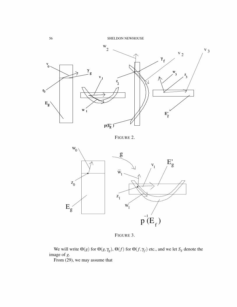
Figures 2 and 3 show some of these objects.

56 SHELDON NEWHOUSE

γf

3z

0z

w3

z2

v 1

w 1

Eg

E’f

γg

p(E’ )g

0v

w2

v 2γ

f

3z

0z

w3

z2

v 1

w 1

Eg

E’f

γg

p(E’ )g

0v

v 3

FIGURE 2.

��

��z0

z1

w0

w1

v1w1

gE’g

Eg

p (E )f

−1

FIGURE 3.

We will write Θ(g) for Θ(g,γg), Θ( f ) for Θ( f ,γ f ) etc., and we let Sg denote theimage of g.

From (29), we may assume that


(134) curv(`−13 ) < ε0 mincurv(γ′′g) < K3

Also, assume that the C2 size of p is bounded above by K4.Consider the maps h = f ◦ p◦g and h = Az3,v3,w3 ◦h◦A−1

z0,v0,w0.

Note that the expressions (34) and (35) give upper bounds for the quantitiesΘ(h),Θ2(h) in terms of Θ( f ),Θ2( f ),Θ(g),Θ2(g), and ang. The only explicit effectof p in these expressions is in the angle term ang. The other effects of the 2-jet of pare absorbed in the constants K1 and C0.

The quantities Θ(h),Θ2(h) are obtained by taking the supremum of Φ(h) andΦ2(h) as z0,v0,w0 vary.

Accordingly, we will first estimate Φ(h),Φ2(h) in terms of Θ( f ),Θ2( f ),Θ(g),Θ2(g),and certain quantities associated with p. For this purpose, we will use various affinemaps to represent h as a composition of maps to which we can apply Lemma 6.4.Once these estimates are obtained, we obtain Theorem 2.5 taking the already indi-cated supremum.

Consider

h = Az3,v3,w3 ◦h◦A−1z0,v0,w0

= Az3,v3,w3 ◦ f ◦ p◦g◦A−1z0,v0,w0

= B1 ◦ f ◦ p◦B2 ◦ g◦B3

where

B1 = Az3,v3,w3 ◦A−1z3,v3,w3

B2 = Az1,v1,w1 ◦A−1z1,v1,w1

B3 = Az0,v0,w0 ◦A−1z0,v0,w0

f = Az3,v3,w3 ◦ f ◦A−1z2,v2,w2

p = Az2,v2,w2 ◦ p◦A−1z1,v1,w1

g = Az1,v1,w1 ◦g◦A−1z0,v0,w0

Thus,

h = F ◦G

58 SHELDON NEWHOUSE

where

F = B1 ◦ f ◦ p, G = B2 ◦ g◦B3

Let us express the various quantities γg,γ f ,γh in the new affine coordinates asfollows.

Set γg = Az0,v0,w0(γg),γh = Az0,v0,w0(γh),γG = B−13 γg = Az0,v0,w0(γg),

γ f = Az2,v2,w2(γ f ),γF = γ f p = G(γh).Note that γg,γG, and γ f are line segments.We wish to apply Lemma 6.4 to F and G.It is easy to see that DFGz0 and DGz0 are diagonal matrices, so (93) and (94) hold.

We now proceed to show that the analog of (90) also holds.First we give some estimates involving the various objects we have defined above.

Lemma 6.6. Let I denote the identity matrix. The matrices DBi satisfy

(135) | I−DB1 | ≤ 2a(v3,v3)a(v3,w3)

(136) | I−DB2 | ≤ 2a(w1,w1)a(v1,w1)

(137) | I−DB3 | ≤ 2a(w0,w0)a(v0, w0)

Proof.Let

u =(

u1u2

), v =

(v1v2

), w =

(w1w2

)be three unit vectors which are pairwise linearly independent, and let β(u,v) denotethe absolute value of the angle between u and v, so that

u = eiβ(u,v)v and set a(u,v) = | sin(β(u,v)) |.Consider the matrix

DAz,u,w ◦DA−1z,v,w.

We have

DAz,u,w =±1

a(u,w)

(w2 −w1−u2 u1

)and


DA−1z,v,w =

(v1 w1v2 w2

).

Thus, assuming β(u,v)≤ π

2 , we have

| I−DAz,u,w ◦DA−1z,v,w | = | DAz,u,w(DA−1

z,u,w−DA−1z,v,w) |

≤ | DAz,u,w || u− v |

≤ | u− v |a(u,w)

=| eiβ(u,v)−1 |

a(u,w)

=

√2(1− cos(β(u,v))

a(u,w)

≤ β(u,v)a(u,w)

≤ 2a(u,v)a(u,w)

.

Similarly,

| I−DAz,u,v ◦DA−1z,u,w | ≤ 2

a(v,w)a(u,v)

.

Now the required estimates of the lemma follow by direct substitution. QED.

Lemma 6.7. Use c ∼ d to mean the quotient cd is bounded above and below by

uniform constants. For any ε0 > 0 there is a K0 > 0 such that if

(138) RuRs ang > K0,

then

(139) a(v1,w1)∼ | p1x |

(140) a(v3, v3)∼J f

| f 21x p1x |

< ε0

(141) a(w0, w0)∼Jg

| g21x p1x |

< ε0,

60 SHELDON NEWHOUSE

and

(142) | G1x |= | g1x |.

Proof.Let

w2 =w2

| w2 |,

and write v2 = av2 +bw2.From the definitions, we have

DAz2,v2,w2(v2) = e1, DAz2,v2,w2(w2) = e2

and

Dp(z1)(v1) = v2.

So, with

e1 =(

10

),

we have (p1x(z1)p2x(z1)

)= Dp(e1)

= DAz2,v2,w2 ◦Dp◦DA−1z1,v1,w1

(e1)= DAz2,v2,w2(v2)= aDAz2,v2,w2(v2)+bDAz2,v2,w2(w2)

=(

ab

).

So, p1x(z1) = a.Since we have uniform bounds above and below for Dp, we have

(143) | p1x(z1) | ∼ ang∼ | ang(v2,w2) | ∼ | ang(v1,w1) | ∼ a(v1,w1).

giving (139).Next, since D f is a diagonal matrix, and

max(| DAz3,v3,w3 |, | DAz2,v2,w2 |)≤√

2C(α)

,


we have

ang(v3, v3) = ang(D f (v2),D f (v2))∼ | tan(ang(D f (v2),D f (v2))) |

=| f2y || f1x |

| tan(ang(v2, v2)) |

=| f2y || f1x |

1| tan(ang(v2,w2)) |

∼| f2y || f1x |

1| p1x |

=J f

| f 21x p1x |

.

Since f is (R,Kuα,Ks

α)−hyperbolic, we have

(144)| f2y || f1x |

≤ (RuRs)−1.

So, we get (140) provided that K0 is large enough.The estimate (141) follows in a similar manner replacing f by g−1 and using the

fact thatJg

| g1x |2∼ J(g)−1

| D(g)−1 |2.

Now, Dg is also diagonal, so, for some constants a,b,a1,b1, we have

DG = DB2 ◦Dg◦DB3

=(

1 a0 b

) (g1x 00 g2y

) (1 a10 b1

)which implies (142).QED.Now we go to the analog of (90) for DF and DG.

Lemma 6.8. For K0 > 1 large enough and RuRs ang ≥ K0, the partial derivativesof F at z1 = G(z0) and G at z0 satisfy

(145) | F2y | ≤ | F1x |and

62 SHELDON NEWHOUSE

(146) | G2y | ≤ (RuRs)−1ang−1| G1x | ≤ | G1x |.

Proof.We first consider the easy case of (146). Indeed, from the definitions, we have

DG = DB2 ◦Dg◦DB3

= DAz1,v1,w1 ◦Dg◦DA−1z0,v0,w0

.

This implies that

| G1x(z0) |= | Dgz0(v0) |, | G2y(z0) |= | Dgz0(w0| w0 |

) |.

Since g is (R,Kuα,Ks

α)−hyperbolic, we have

| G1x(z0) |> Ru,

and, up to a constant C = C(| Dp |, | Dp−1 |),

| Dgz0(w0| w0 |

) | =(| D(g−1)z1(

w1| w1 |

|)−1

≤ (Rs | tan(ang(v1,w1)) |−1

≤ C(Rs ang)−1

≤ C(Rs ang)−1 | G1x(z0) || G1x(z0) |

≤ C(RuRs)−1ang−1| G1x(z0) |giving (146).Next, we go to (145).We have

F = B1 ◦ f ◦ p.

Write

DB1 =(

b11 b12b21 b22

).

Then, b12 = 0 and b22 = 1. Also, D fz2 is a diagonal matrix and Dpz1 is a lowertriangular matrix.

Hence,


(147) F1x = b11 f1x p1x

and

(148) F2y = f2y p2y.

Now | p2y | is bounded, and, for K0 large, (135) gives that DB1 is close to theidentity I. Hence, for K0 large, we have | b11 |> 1

2 .Thus, for some constant K > 0 and K0 large enough, we have

| F2y || F1x |

≤ K(RuRs)−1 ang−1 ≤ KK0

≤ 1

which is (145). QEDThe next lemma gives an estimate for the curvature of the curve γ f p (or its

reparametrization γ f p) in terms of Θ(g).Note that γ f p = g(γh) which is a part of the curve g(γg).

Lemma 6.9. There is a constant C(α) > 0 such that

(149) curv(γ f p)≤C(α)Θ(g)| g(γg) |

Proof.As usual, we will write C(α) for possibly different functions of α.We write γg as the graph of a function y = ρ(x) = y0 for x ∈ [α0,β0]. Then,

Dρ(x) = D2ρ(x) = 0 for all x. By the graph transform formula, we have g(γg) is thegraph of the function Γ(g,ρ) defined by

(150) Γ(g,ρ) = g2 ◦ (1,ρ)◦ ([g1 ◦ (1,ρ)]−1,

where (1,ρ) denotes the function x→ (x,ρ(x)).The curvature curv(γ f p) is proportional to | D2Γ(g,ρ) |, so it suffices to estimate

this last quantity.Let u(x) = [g1 ◦ (1,ρ)]−1(x).Then, differentiating the above formula, we get

DΓ(g,ρ) = g2x(ux,ρux)Du(x)+g2y(ux,ρux)Dρ(ux)Du(x)= g2xDu(x)+g2yDρ(ux)Du(x)

64 SHELDON NEWHOUSE

D2Γ(g,ρ) = g2xxDu(x)Du(x)+g2xyDu(x)Dρ(ux)Du(x)

+g2yxDu(x)Dρ(ux)Du(x)+g2yyDρ(ux)Dρ(ux)Du(x)Du(x)

+g2xD2u(x)+g2yD

2ρ(ux)Du(x)Du(x)

+g2yDρ(ux)D2u(x)(151)

We can compute formulas for Du,D2u in terms of g,ρ by differentiating the for-mula g1(ux,ρux) = x twice and solving for Du,D2u.

We get

(152) Du(x) =[g1x(ux,ρux)+g1y(ux,ρux)Dρ(ux)

]−1

and

D2u(x) = −Du(x)[g1xx(Du(x))2 +2g1xyDρ(ux)Du(x)Du(x)

+g1yy(Dρ(ux))2Du(x)2 +g1y(Du)2D2ρ(ux)

].

Now, we have that

| γg || g(γg) |

∼ 1| g1x |

.

Hence, computing all partial derivatives at points x ∈ [α0,β0] we have, for eachi = 1,2,

(153) max(| gixx || g1x |2

,| gixy || g1x |2

,| giyy || g1x |2

)≤C(α)Θ(g)| g(γg) |

,

(154) | Du(x) | ≤ 1| g1x |(1−α| Dρ |)

=1

| g1x |,

(155) max(| g2x || g1x |

,| giy || g1x |

)≤ α < 1,

(156) Dρ = 0, D2ρ = 0.

Combining these estimates proves Lemma 6.9. QED.Next, we have a simple estimate which we will be used in the proof of estimate

(168) below.


Lemma 6.10. Let ρ1,ρ2 : [a,b]→R be C2 functions such that ρ1(a)= ρ2(a),ρ1(b)=ρ2(b) and there are constants 0 < K1 < K2 < K3 such that, for all x ∈ [a,b],

(157) | D2ρ1(x) | ≤ K1, | D2ρ2(x) | ≤ K3,

and

(158) D2ρ2(x) <−K2.

Then, letting φ = ρ1−ρ2 and

M = maxx∈[a,b]

| φ(x) |,

we have

(159)K2−K1

8≤ M

(b−a)2 ≤K1 +K3

8.

Moreover, there is a unique c ∈ (a,b) such that Dφ(c) = 0.Let x1,x2 be in the same interval of [a,b] \ {c}, and assume there is a constant

K > 0 such that | x1− x2 | ≤ K| x1− c |.Then,

(160)| Dφ(x2) || Dφ(x1) |

≤ exp(

K(K1 +K3)K2−K1

).

Proof. Let C1 = K2−K1, C2 = K1 +K3.We have

φ(a) = φ(b) = 0,

and

(161) 0 < C1 ≤ D2φ(x)≤C2

for all x ∈ [a,b], and C1 < C2. .Also,

M = |minx∈[a,b] φ(x) |=− minx∈[a,b]

φ(x).

Then, there is a unique c ∈ (a,b) such that Dφ(c) = 0.We place the graph of φ between two parabolas to get our required estimate (159).Thus, consider the two quadratic functions

66 SHELDON NEWHOUSE

qi(x) =Ci

2(x− c)2−M

for i = 1,2.Since the functions qi,φ each have c as a unique minimum, our assumptions

(157), (158) together with (161 imply that

(162) q1(x)≤ φ(x)≤ q2(x)

for all x ∈ [a,b].Letting ci > c be the unique point such that qi(ci) = 0 we have

ci− c =√

2MCi

.

Also, since the distance between the zeroes of qi is 2(ci− c), (162) implies that

2(c2− c)≤ b−a≤ 2(c1− c),or, √

2MC2

≤ b−a2

≤√

2MC1

.

This is equivalent to (159).Next, we obtain some estimates on the ratio of angles between the vectors (1,Dρ1(x))

and (1,Dρ2(x)) at certain different points x1,x2.For two vectors v1,v2 let ang(v1,v2) denote the angle between the vectors v1,v2

as defined in (9). Letting e1 =(

10

), set αi = αi(x) = ang((1,Dρi(x)),e1).

Then, Dφ(x) = tan(α1(x))− tan(α2(x)).Assume that | tan(α1(x)) | ≤ α < 1, | tan(α2(x)) | ≤ 1.Using

tan(α1−α2) =tan(α1)− tan(α2)

1+ tan(α1) tan(α2),

we get

Dφ(x) = (1+ tan(α1) tan(α2))(tan(α1−α2)).This gives

(163) 1−α≤ | Dφ(x) || tan(α1−α2) |

≤ 1+α.


Next, we proceed to prove (160). We have to estimate the quotient

| Dφ(x2) || Dφ(x1) |

where | x1− x2 |< | x1− c |.We have 0 <C1 ≤D2φ(x)≤C2, c is the unique minimum of φ in [a,b], and Dφ(x)

is strictly increasing for c < x < b.We have that x1 and x2 must lie on the same side of c. Assume first that c < x1 <

x2 < b.Then,

logDφ(x2)Dφ(x1)

=D2φ(τ)Dφ(τ)

(x2− x1)

≤ C2

Dφ(x1)(x2− x1).

Also,

Dφ(x1) = Dφ(x1)−Dφ(c) =Z x1

cD2

φ(s)ds

≥ C1(x1− c).

Hence,

(164) logDφ(x2)Dφ(x1)

≤ C2(x2− x1)C1(x1− c)

or, since | x2− x1 | ≤ K| x1− c |, we have

(165)| Dφ(x2) || Dφ(x1) |

≤ exp(

C2| x2− x1 |C1| x1− c |

)≤ exp

(KC2

C1

).

Using similar techniques, we can handle the remaining cases c < x2 < x1 < b, a <x1 < x2 < c, a < x2 < x1 < c. This proves Lemma 6.10. QED.

Let γh = Az0,v0,w0(γh),γF = γ f p = G(γh).

Lemma 6.11. There is a constant K > 0 such that

(166)K−1

ang≤| γ f p || γ f |

≤ Kang

,

and, for any point τ ∈ γ f p, we have

68 SHELDON NEWHOUSE

(167)| p1x(τ) || p1x(z1) |

≤ exp

(KΘ(g)| γ f |

2

ang5 +K| γ f |ang2

)as well as

(168) K−1ang≤ | p1x(τ) | ≤ K ang

Proof.Using

| γ f |ang2 =

(| γ f |

2

ang5

) 12

ang12 and | γ f | ∼ | γ f |,

we see that (27) implies that the right side of (167) is bounded. This, togetherwith (143) and (167), implies (168).

Hence, we need only concern ourselves with (166) and (167).Consider the curve p(g(γg))) and the left and right boundary curves of E f . For

ease of notation, let us denote these by

γ1 = ∂le f t(E f ), γ2 = ∂right(E f ), γ3 = p(g(γg))).

For i = 0,1,2,3, let zi = (xi, yi) be such that

γ1

\γ3 = {z0, z3}, γ2

\γ3 = {z1, z2}.

We assume that y3 < y2 < y1 < y0.From Lemma 6.10, we may think of the curves ∂le f t(E f ),∂right(E f ) as lines, and

the curve γ3 as a quadratic curve of curvature greater than the parabolic curvatureof the map p.

Let `0 denote the tangent line to γ1 at z0 and let θ denote the angle between thisline and the vertical direction.

Let zc be the point on γ3 whose distance to the line `0 is a maximum.Choosing rotated coordinates ζ(x,y) = (ξ(x,y),η(x,y)) with

ξ = x cos(θ)− y sin(θ)η = x sin(θ)+ y cos(θ),

we have that ξ = 0 corresponds to the direction of `0.Letting (ξi,ηi) = ζ(zi) we have η3 < η2 < η1 < η0 and there are C2 functions

ξ = ρi(η), η3 ≤ η≤ η0 such that


γi = {(ρi(η),η), 0≤ i≤ 3, η3 ≤ η≤ η0}.Further,

(169) ρ1(η0) = ρ3(η0), ρ1(η3) = ρ3(η3), Dρ1(η0) = 0.

Let

K1 = maxη| D2ρ1(η) |, K2 = max

η| D2ρ2(η) |, K3 = min

η| D2ρ3(η) |.

The curvature, curvγ(z), of a C2 curve γ : ξ = ρ(η) at the point z = (ρ(η),η)satisfies

(170) curvγ(z) =| D2ρ(η) |

(1+Dρ(η)2)32.

Letting K4 be an upper bound for | η0−η3 |, since Dρ1(η0) = 0, we have

(171) | Dρ1(η) | ≤ K1| η0−η3 | ≤ K1K4

Now, (29) gives that, for i = 1,2,

(172) curv(γi) < ε0 mincurv(γ3).

We claim that if

(173) ε0(1+K21 K2

4 )32 <

12,

then

(174) K1 = maxη| D2ρ1(η) | ≤ 1

2min

η| D2ρ3(η) |= 1

2K3.

Indeed, for η, η ∈ [η3,η0], we have

curvγ1(ρ1(η),η)≤ ε0 curvγ3

(ρ3(η), η).

Thus, (171) and (173) give

70 SHELDON NEWHOUSE

| D2ρ1(η) | =| D2ρ1(η) |(1+Dρ1(η)2)

32

(1+Dρ1(η)2)32

≤ ε0| D2ρ3(η) |(1+Dρ1(η)2)

32

(1+Dρ3(η)2)32

≤ ε0 | D2ρ3(η) |(1+K21 K2

4 )32

≤ 12| D2ρ3(η) |.

Since η, η ∈ [η3,η0] are arbitrary, we get (174).Consider the curve γ f p.Since Dp is bounded above and below, so is Dp. Hence,

(175) | γ f p | ∼ | p(γ f p) |.

The curve p(γ f p) has the parametrization

p(γ f p) = {(ρ3(η),η) : η1 ≤ η≤ η0}.Since z0, z1 are the boundary points of p(γ f p) and the slopes of the tangent vectors

to p(γ f p) are greater than one, we have

| p(γ f p) | ∼ | η1−η0 |.By the Mean Value Theorem there is a η5 ∈ (η1,η0) such that

| ξ0−ξ1 |= | Dρ3(η5) || η0−η1 |.Let ` f denote the horizontal line through z1 (in the (ξ,η)−coordinates), and let

z4 denote its intersection with ∂le f t(E f ). Let z4 = (ξ4,η1).There is a point η6 ∈ (η1,η0) such that

| ξ0−ξ4 |= | Dρ1(η6) || η0−η1 |,Let c ∈ (η3,η0) be the unique real number such that Dρ3(c) = 0.Using (29), we choose ε0 small enough so that

K1(1+height(Q)) <12

K3.

Then


| ξ0−ξ4 | = | Dρ1(η6) || η0−η1 |= | Dρ1(η5)+Dρ1(η6)−Dρ1(η5) || η0−η1 |≤ K1| η0−η1 |+K1| η0−η1 |2

≤ K1(1+height(Q))| η0−η1 |

≤ 12

K3| η0−η1 |

≤ 12| Dρ3(η5) || η0−η1 |

=12| ξ0−ξ1 |

Then, using

(176) | ξ0−ξ1 |− | ξ0−ξ4 | ≤ | γ f | ≤ | ξ0−ξ1 |+ | ξ0−ξ4 |,we get

(177)12≤

| γ f || ξ1−ξ0 |

≤ 32.

Since | γ f p | ∼ | η0−η1 |, this gives

| γ f p || γ f |

∼ 1| Dρ3(η5) |

,

so, for (166), it suffices to show

(178) | Dρ3(η5) | ∼ ang = a(v2,w2).

Using (26) and (29) and a appropriately small ε0, we can find a constant K5 > 0such that

| η0−η1 | ≤ K5| η1− c |.Then, (178) follows from Lemma 6.10.We proceed to prove (167).Using (143) and

1− | p1x(τ)− p1x(z1) || p1x(z1) |

≤ | p1x(τ) || p1x(z1) |

≤ 1+| p1x(τ)− p1x(z1) |

| p1x(z1) |,

it suffices to prove that

72 SHELDON NEWHOUSE

(179) | p1x(τ)− p1x(z1) | ≤ K

(Θ(g)| γ f |

2

ang4 +| γ f |ang

)for any point τ ∈ γ f p.We have

p = Az2,v2,w2 ◦ p◦A−1z1,v1,w1

,

and

p(z1) = p(z1) = z2.

Since Ax2,v2,w2, D2 p, and A−1z1,v1,w1

are bounded, we get

(180) |(

p1x(τ)p2x(τ)

)−(

p1x(z1)p2x(z1)

)| ≤ K| τ− z1 |.

Now, τ is in the Az1,v1,w1−image of the curve γ f p. Note that | γ f p |= | γ f p | sincethese are arclengths of curves which differ only by reparametrization and a rotationof coordinates.

If we show that there is a constant K1 > 0 such that for every unit tangent vectorv to γ f p,

(181) | DAz1,v1,w1(v) | ≤ K1

(Θ(g)| g(γg) |

| γ f p |ang

+1

),

then, it will follow that

(182) | τ− z1 | ≤ K1| γ f p |

(Θ(g)| g(γg) |

| γ f p |ang

+1

).

Using (166) and the fact that | g(γg) | ∼ ang,we get

(183) | τ− z1 | ≤ K1

(Θ(g)| γ f |

2

ang4 +| γ f |ang

).

This will imply (179), completing the proof of Lemma 6.11.So, let v be a unit tangent vector to the curve γ f p at some point. By Lemma 6.9

the curvature of γ f p is bounded by C(α) Θ(g)| g(γg) |

.


Hence, we have that

| v− v1 | ∼ | tan(ang(v,v1)) | ≤C(α)Θ(g)| γ f p || g(γg) |

,

and, from (78), we have

| DAz1,v1,w1 | ≤K

ang.

This gives, with e1 =(

10

),

| DAz1,v1,w1(v) | = | DAz1,v1,w1(v− v1)+DAz1,v1,w1(v1) |= | DAz1,v1,w1(v− v1)+ e1 |

≤ K| v− v1 |ang

+1

≤KC(α)Θ(g)| γ f p || g(γg) |ang

+1

and we simply take

K1 = max(KC(α),1).

Let us return to the verification of (34) and (35).We can now apply Lemma 6.4.By (106) and (107) we have

(184) Φ(h)≤Φ(F)exp(

Ψ2(G)| γh || γG |

)+Φ(G)

| γh || γG |

and

Φ2(h) ≤ Φ2(F)ε22(G)exp(

Ψ2(G)| γh || γG |

)+Φ2(G)

| γh || γG |

= Φ2(F)JG

| G1x |2exp(

Ψ2(G)| γh || γG |

)+Φ2(G)

| γh || γG |

(185)

From our previous results and definitions, we have

F = B1 ◦ f ◦ p,

74 SHELDON NEWHOUSE

(186) | F1x |= | b11 || f1x p1x |,

(187) | G1x |= | g1x |,

(188) | h1x |= | b11 || f1x p1xg1x |.Since, a(v3, v3) is small, we have

Φ(F) ≤ | DB1 |Φ( f p)

≤ 1+K1a(v3, v3)1−K1a(v3, v3)

Φ( f p)

≤ (1+3K1a(v3, v3))Φ( f p)(189)≤ (1+Ka(v3, v3))Φ( f p)(190)

(191)

and

(192) Φ2(F)≤ KΦ2( f p).

Letting Sg = g(γg), we have

(193) | g1x || γg | ∼ | Sg |,and

(194) | γh | ∼| γ f |

| g1x p1x |,

so,

(195)| γh || γg |

∼| γh || γG |

≤ K5| γ f |

| p1x || Sg |

Let us estimate Φ( f p) and Φ2( f p).We know that p1y(z2) = p1y = 0, and

| p2x |, | p2y |< KUsing (96)–(98) with h = f p and ε22( f )≤ 1, we get


Φ11( f p) ≤ Φ11( f )| p1x || γ f p || γ f |

+2KΦ12( f )| γ f p || γ f |

+KΦ22( f )| γ f p |

| p1x || γ f |

+2maxi

| pixx || p1x |

| γ f p |

Φ12( f p)≤Φ12( f )K| γ f p || γ f |

+Φ22( f )K| γ f p |

| p1x || γ f |+ 2max

i

| pixy || p1x |

| γ f p |

Φ22( f p)≤Φ22( f )K

| p1x || γ f p || γ f |

+2maxi

| piyy || p1x |

| γ f p |

Using Lemma 6.11, we have

1| p2

1x |∼ 1| p1x(τ1) || p1x(τ) |

∼ 1ang2 ,

so,

(196) Φ( f p)≤Φ( f )exp

(K

Θ(g)| γ f |2

ang5 +K| γ f |ang2

)+K

Φ2( f )ang2 +

K| γ f |ang2

and

(197) Φ2( f p)≤ KΦ2( f )ang2 +

K| γ f |ang2

Now,

| D2 p | ≤ K

and

a(v3, v3)≤ K| f2y || f1x p1x |

∼ J f| f 2

1x p1x |Since | J f | ∼ | J f |, | f1x | ∼ | f1x |, | γ f | ∼ | γ f |, | p1x | ∼ a(v2,w2), we have

a(v3,v3)≤ KJ?( f ,γ f )

ang,

or

76 SHELDON NEWHOUSE

(198) 1+a(v3,v3)≤ exp(

KJ?( f ,γ f )

ang

).

This gives

Φ(F) ≤ Φ( f )exp

(K

J?( f ,γ f )ang

+KΘ(g)| γ f |

2

ang5 +K| γ f |)ang2

)

+ KΦ2( f )ang2 +K

| γ f |ang2(199)

and

(200) Φ2(F)≤ KΦ2( f )ang2 +K

| γ f |ang2

Now, G = B2 ◦ g◦B3, B3 is bounded, and

| B2 | ∼1

ang.

Hence, we get

Φ(G) ≤(

1+Ka(w1, w1)a(v1,w1)

)Φ(g)

(1+K

a(w0,w0)a(v0,w0)

)2

≤ Kang

Φ(g),

and

JG ≤ KJg

ang.

Now,

DB3 =(

1 a0 b

) (xy

)where | b | ≤ K, and

| a | ≤ Ka(w0, w0)≤ K min(Jg

| g21x p1x |

,C(α)).

By (30), this last quantity is less than 1.Since γG = B−1

3 γg, we have


| γG | ∼ | γg |.

Further, if z0 = (x0,y0), and we set G = g◦B3, we get

G = g◦B3(x,y) = (g1(x0 + x+ay,y0 +by), g2(x0 + x+ay,y0 +by))

and

| G1x | = | g1x || Gixx | = | gixx || Giyx | ≤ (| gixx |a+ | gixy |b)

| Giyy | ≤ (| gixx |a2 +2| gixy |ab+ | giyy |b2).

| D2G | ≤ | DB2 || D2G | ≤ K| p1x |

| D2G |.

Setting

J1 = J1(g) =Jg

| g21x p1x |

we have

(201) Ψ2(G)≤ K| p1x |

Ψ2(g)∼ Kang

Ψ2(g)

and

Φ2(G) ≤ KΦ(g)| p1x |

max(| a |, | a |2)+KΦ2(g)| p1x |

≤ KΦ(g)J1

| p1x |+

KΦ2(g)| p1x |

.(202)

Since g = Az1,v1,w1 ◦g◦A−1z0,v0,w0

and the matrices DAz1,v1,w1,DA−1z0,v0,w0

are bounded,we get

(203) Ψ2(g)≤ KΨ2(g) and Jg ≤ KJg.

Applying (106) gives

78 SHELDON NEWHOUSE

Φ(h) ≤ Φ(F)exp(

Ψ2(G)| γh || γG |

)+Φ(G)

| γh || γG |

≤ Φ(F)exp

(K2

Ψ2(g)| p1x |

| γh || γg |

)+K2

Φ(g)| p1x |

| γh || γg |

Since, | p1x | ∼ a(v2,w2) = ang, taking the supremum over all z0,v0,w0 gives(34).

To estimate Θ2(h), we use (107) and the above to get

Φ2(h) ≤ Φ2(F)| JG || G1x |2

exp(Ψ2(G)| γh || γG |

)+Φ2(G)| γh || γG |

≤ K

(Φ2( f )

| p1x |2+

| γ f || p1x |2

)| Jg |

| p1x || g1x |2exp(

Ψ2(G)| γh || γG |

)+ K

Φ(g)J1

| p1x || γh || γg |

+ KΦ2(g)| p1x |

| γh || γg |

≤ K

(Φ2( f )

| p1x |2+

| γ f || p1x |2

)J1 exp

(K

Ψ2(g)| p1x |

| γh || γg |

)

+ KΦ(g)J1

| p1x || γh || γg |

+ KΦ2(g)| p1x |

| γh || γg |

Using | p1x | ∼ ang, and taking the supremum over z0,v0,w0, we get (35).This completes the proof of Theorem 2.5. QED


7. PROOFS OF THEOREMS 2.6, 2.7, AND 2.8

7.1. Proof of Theorem 2.6. Let h = f ◦ p◦g be the map in question.Note that (36) implies that

(204) J1( f ,γ f ) =J f

ang| f1x |2<| γ f |ang2 .

Now, using (31), (34), (204), and setting

(205) ν0 =Θ2( f )ang2 +

Θ(g)| γ f |2

ang5 +2| γ f |ang2 +

Θ(g)ang

| γh || γg |

,

we have

(206) Θ(h)≤Θ( f )exp(K1ν0)+K1ν0.

From (37) we have

ang < 1 and| γ f |ang2 < K2| Sg |−δ2 | γh |

| γg |< 1.

Hence, we have

| γ f |2

ang4 <| γ f |ang2 ,

and

Θ(g)ang5 | γ f |

2 <Θ(g)ang

| γ f |ang2 ≤

Θ(g)ang

K2| Sg |−δ2 | γh || γg |

.

Also, by (38) and (39), we have

Θ(g)ang

≤ K22 | Sg |1−δ1−1−δ2 = K2

2 | Sg |−δ1−δ2 > 1.

Putting these estimates together with (205) and (40), we get

ν0 ≤ Θ2( f )ang2 +4

(K3

2 | Sg |−δ1−2δ2)( | γh |

| γg |

)

≤ ν3 =Θ2( f )ang2 +

(| γh || γg |

)1−δ3

80 SHELDON NEWHOUSE

as required in (41). QED.

7.2. Proof of Theorem 2.7. From (35), we have the following estimate for Θ2(h).

Θ2(h) ≤ K1

(Θ2( f )ang2 +

| γ f |ang2

)J1(g,γh)exp

(Θ(g)ang

| γh || γg |

)

+K1Θ(g)J1(g,γh)

ang| γh || γg |

+K1Θ2(g)ang

| γh || γg |

.

Using

Θ(g)≤ L1, exp

(Θ(g)ang

| γh || γg |

)≤ L2,

we get

Θ2(h) ≤ K1

(Θ2( f )ang2 +

| γ f |ang2

)J1(g,γh)L2

+K1L1J1(g,γh)

ang| γh || γg |

+K1Θ2(g)ang

| γh || γg |

.(207)

As we noted above, from (37) we have

(208)| γ f |ang2 < K2| Sg |−δ2 | γh |

| γg |.

Using (37), (39), (45),(46), and (48) we get


Θ2(h) ≤ K1L2Θ2( f )ang2 J1(g,γh)+K1L2K2| Sg |−δ2 | γh |

| γg |J1(g,γh)

+K1L1J1(g,γh)

ang| γh || γg |

+K1Θ2(g)ang

| γh || γg |

≤ K1L2Θ2( f )ang2 J1(g,γh)+2K3

3J1(g,γh)

ang| γh || γg |

+K1Θ2(g)ang

| γh || γg |

≤ K1L2Θ2( f )ang2 J1(g,γh)+

(12

+K1Θ2(g)ang

)| γh || γg |

≤ K1L2J1(g,γh)

ang2 Θ2( f )+

12

+K1| γg |

1−δ3

ang

| γh || γg |

≤ K1L2J1(g,γh)

ang2 Θ2( f )+34

(| γh || γg |

)1−δ3

≤ K1L2Jg

ang3| g1x |2Θ2( f )+

34

(| γh || γg |

)1−δ3

and, hence,

(209) Θ2(h)≤ K3Jg

ang3| g1x |2Θ2( f )+

34

(| γh || γg |

)1−δ3

.

Case 1: h = f ◦ p◦g is a bcc map.Then, by (39), (44), (47) and the fact that ang < 1, we have (for δ2,δ3 appropri-

ately small)

82 SHELDON NEWHOUSE

Θ2( f ) < | γ f |1−δ3

<

(| γ f |

ang2−2δ2

)1−δ3

=( | γ f |

ang2

)1−δ3

ang2δ2(1−δ3)

≤ K1−δ32 | Sg |−δ2(1−δ3)ang2δ2(1−δ3)

(| γh || γg |

)(1−δ3)

≤ K1−δ32 | Sg |−δ2(1−δ3)(K2| Sg |)2δ2(1−δ3)

(| γh || γg |

)(1−δ3)

= K(1−δ3)(1+2δ2)2 | Sg |δ2(1−δ3)

(| γh || γg |

)(1−δ3)

<

(| γh || γg |

)(1−δ3)

So, using (44), (45), and (209), we get (55).Case 2: h = f ◦ p◦g = f1 ◦ p◦g1 ◦ p◦g where f1 and f = f1 ◦ p◦g1 are cc maps

of rank less than that of h, and g def= g1 ◦ p◦g is a bcc map.Using induction, we may assume that

(210) Θ2( f )≤

(| γ f || γg1

|

)1−δ3

.

Let ang denote the angle of the map g.We first assert that

(211) inequality (209) holds with f replaced by f .

To see this we observe that

(1) (209) was obtained using the estimates (37), (39), (45), (46), and (48) forthe maps f , p, and g,


(2) using (54) to replace the right hand side of (37) we see that all of theseconditions are unchanged in replacing f by f .

Continuing with our proof, we use (54) and the left side of (39) to get

(212) K2| Sg |−δ2 | γh || γg |

>| γ f |ang2 =

| γ f || γg1

|| γg1

|ang2

and

(213) | Sg |−δ2 < Kδ22 ang−δ2.

So,

| γ f || γg1

|< K2| Sg |−δ2 | γh |

| γg |ang2

| γg1|

< K1+δ22

| γh || γg |

ang2−δ2

| γg1|

≤ K1+δ23

| γh || γg |

ang2−δ2

| γg1|

.

From Case 1, we have that

(214) Θ2(g)≤

(| γg || γg |

)1−δ3

,

Using (209) with f replaced by f , and appropriately defining small numbersδ4,δ5, we have

84 SHELDON NEWHOUSE

Θ2(h) ≤ K3Jg

ang3| g1x |2Θ2( f )+

34

(| γh || γg |

)1−δ3

≤ K3Jg

ang3| g1x |2

(| γ f || γg1

|

)1−δ3

+34

(| γh || γg |

)1−δ3

≤ K3Jg

ang3| g1x |2

| γh || γg |

K1+δ23 ang2−δ2

| γg1|

1−δ3

+34

(| γh || γg |

)1−δ3

≤K2+δ4

3 ang2−δ5Jg

ang3| g1x |2

(| γh || γg |

1| γg1

|

)1−δ3

+34

(| γh || γg |

)1−δ3

≤K3

3 Jg

ang2| g1x |2

(| γh || γg |

1| γg1

|

)1−δ3

+34

(| γh || γg |

)1−δ3

≤

(| γh || γg |

)1−δ3

where we have used (49) for the bcc map g1 ◦ p◦g.This completes the proof of (55).Now, assume that h is an ecc map.From (35), (37), (42), (43), and (45) we can write (207) as

Θ2(h) ≤ K3Θ2( f )ang2 J1(g,γh)+K2

3 | Sg |−δ2 | γh || γg |

J1(g,γh)

+K3J1(g,γh)

ang| γh || γg |

+K3Θ2(g)ang

| γh || γg |

(215)

The upper bound Θ(g)≤ L1 gives us that

exp(−L1)≤| g1x(z) || g1x(w) |

≤ exp(L1)

for any z,w ∈ γg, so

exp(−L1)| Sg | ≤ | g1x || γg | ≤ | Sg |exp(L1).Also, repeating (213), we have


| Sg |−δ2 < Kδ22 ang−δ2

and, setting K3 = max(K2+δ22 exp(L1),3), we have

1| g1x |

| γ f |ang

=| γ f |ang2

ang| g1x |

≤ K2| Sg |−δ2 ang| g1x |

| γh || γg |

≤ K2| Sg |−δ2 angSg

exp(L1)| γh |

≤ K3ang−δ2| γh |.So, we may assume

(216) | γ f | ≤ K3| g1x || γh |ang1−δ2,

(217) ang≤ K3| g1x || γg |,

(218) Θ2( f ) < | γ f |1−δ3,

and

(219) Θ2(g) < | γg |1−δ3.

From (50), (51), and (52),we have

(220)Jg

ang2+δ4| g1x |1+δ3<

13K3

,

(221)Jg| γh |

δ3

ang3| g1x |<

13K3

,

and

(222)1

ang

(| γh || γg |

)δ3

<1

3K3.

86 SHELDON NEWHOUSE

From (37) and (39), we have

ang < K2| Sg |

and

| Sg |< 1,

so, in particular,

(223) ang < K2| Sg |δ2.

Using (215)–(223), writing a � b to mean a ≤ K3b, and setting δ4 = δ2 + δ3−δ2δ3, we get

Θ2(h) �| γ f |

1−δ3J1(g,γh)ang2 +

J1(g,γh)ang

| γh || γg |

+| γg |

1−δ3

ang| γh || γg |

�(| g1x || γh |ang1−δ2)1−δ3J1(g,γg)

ang2 +J1(g,γh)

ang| γh || γg |

+1

ang

(| γh || γg |

)δ3

| γh |1−δ3

� (| g1x || γh |)1−δ3Jg

ang2+δ4| g1x |2+

Jg

ang2| g1x |2| γh || γg |

+1

ang

(| γh || γg |

)δ3

| γh |1−δ3

� (| γh |)1−δ3Jg

ang2+δ4| g1x |1+δ3+

Jgang3| g1x |

| γh |

+1

ang

(| γh || γg |

)δ3

| γh |1−δ3

≤ | γh |1−δ3

This completes the proof of Theorem 2.7. QED.


7.3. Proof of Theorem 2.8. We apply the exponential increment Lemma 5.1 andthe estimates of Theorems 2.6 and 2.7.

Let a0 = K4 exp(K4), b0 = b1 = c0 = c1 = K4, ai = Θ(hi) for i≥ 1, and bi = ci =K4ξi for i≥ 2.

Then,

a0 ≤ b0exp(b0),and, by (58) and Theorem 2.6 we have

a1 ≤ Θ(h0)exp

K1Θ2(h0)ang2

1+K1

| γh1|

| γg1|

1−δ3

+K1Θ2(h0)ang2

1+K1

| γh1|

| γg1|

1−δ3

≤ a0exp(K4)+K4

= a0exp(b1)+b1

Further, from (57), we have Θ(g0)≤ b0 ≤ b0 exp(b0) = a0.Then, by Theorem 2.6, Theorem 2.7, and (59), for i≥ 2, we have

ai ≤ ai−1exp(K1ν3)+K1ν3

≤ ai−1exp

K1Θ2(hi−1)

ang2i

+K1

(| γhi

|| γgi

|

)1−δ3

+K1Θ2(hi−1)

ang2i

+K1

(| γhi

|| γgi

|

)1−δ3

≤ ai−1exp

K1

ang2i

(| γhi−1

|| γgi−1

|

)1−δ3

+K1

(| γhi

|| γgi

|

)1−δ3

+K1

ang2i

(| γhi−1

|| γgi−1

|

)1−δ3

+K1

(| γhi

|| γgi

|

)1−δ3

≤ ai−1exp(bi)+bi.

So, Lemma 5.1 applies to give (60) as required. QED.

REFERENCES

[1] M. Benedicks and L. Carleson. The dynamics of the Henon map. Annals of Math., 133:73–169,1991.

88 SHELDON NEWHOUSE

[2] W. de Melo and S. van Strien. One-Dimensional Dynamics, volume 25 of Ergebnisse der Math-ematik. Springer-Verlag, New York, 1991.

[3] M. Hirsch and C. Pugh. Stable manifolds and hyperbolic sets. Proc. AMS Symp. Pure Math.,14, 1970.

[4] M. V. Jakobson. Absolutely continuous invariant measures for one-parameter families of one-dimensional maps. Comm. Math. Phys., 81:39–88, 1981.

[5] M. V. Jakobson and S. E. Newhouse. A two dimensional version of the folklore theorem. Amer-ican Math. Soc. Translations, Series 2, 171:89–105, 1996.

[6] M. V. Jakobson and S. E. Newhouse. Asymptotic measures for hyperbolic piecewise smoothmappings of a rectangle. Asterisque, 261:103–159, 2000.

[7] M. Misiurewicz. Absolutely continuous invariant measures for certain maps of the interval.Publ. Math. IHES, 53:17–51, 1981.

[8] L. Mora and M. Viana. Abundance of strange attractors. Acta Mathematica, 171:1–71, 1993.[9] S. Newhouse. Cone-fields, domination, and hyperbolicity. In Michael Brin, Boris Hasselblatt,

and Yakov Pesin, editors, Modern Dynamical Systems and Applications, pages 419–432. Cam-bridge Press, 2004.

[10] J. Palis and J-C. Yoccoz. Implicit formalism for affine-like maps and parabolic composition.In H W Broer, B Krauskopf, and G Vegter, editors, Global Analysis of Dynamical Systems:Festschrift dedicated to Floris Takens for his 60th birthday, pages 67–88, Bristol and Philadel-phia, 2001. Institute of Physics Publishing.

[11] J. Jr. Palis and J.-C. Yoccoz. Non-Uniformly Hyperbolic Horseshoes Arising from Bifurcationsof Poincare Heteroclinic Cycles. ArXiv Mathematics e-prints, April 2006.

[12] Ja. G. Sinai. Gibbs measures in ergodic theory. Russian Math. Surveys, 27:21–69, 1972.[13] Ya.G. Sinai. Topics in Ergodic Theory. Number 44 in Princeton Mathematical Series. Princeton

University Press, 1994.[14] D. Wang and L.S. Young. Strange attractors with one direction of instability. Comm. Math.

Phys., 218:1–97, 2001.


8. GLOSSARY

INDEX OF SPECIAL SYMBOLS AND NOTATIONS

Numbers on right indicate the page where the term is defined

Notation Definition Page

Jγ f (z) 6Az,v,w 11`v(w) 15γ(t) 6fz,v,w 12curv(γ) maximum curvature along γ 6f � p� g 14lw(E) 15mC 9f � g g Markov precedes f 7compatible parametrized rectangles 6full-height subrectangle 6full-width subrectangle 6full-width(height) curve 6parametrized rectangle 6rectangle curvlinear rectangle 6standard rectangle linear rectangle 6v2 normal vector to w2 at z2 55v3 D f (v2) normalized 55w0 Dg−1(w1) normalized 55w1 normal vector to v1 at z1 55γ[z0,z1] polygonal approximation of [z0,z1] 50a(v,w) | sin(ang(v,w)) | 52v0 unit vector in Ku

α(z0) 55v1,v2,v3 successive images of v0 55w0,w1,w2 successive pre-images of w3 55w3 unit vector in Ks

α(z3) 55w f (z0,z1) min length of some horizontal line segments 51z0,z1 z0 ∈ γh,z1 = g(z0) 55z2,z3 z2 = p(z1),z3 = f (z2) 55

Ksα 8

Kuα 8

(R,α)−hyperbolic 10

90 SHELDON NEWHOUSE


(R,α,z)−hyperbolic 11<,> Euclidean inner product 5DB1 derivative of Az3,v3,w3 ◦A−1

z3,v3,w358

DB2 derivative of Az1,v1,w1 ◦A−1z1,v1,w1

58DB3 derivative of Az0,v0,w0 ◦A−1

z0,v0,w058

H0�H1 concatenation 23J?(g,γ) 17J1(g,γ) 17J f 17K− parabolically 13, 14Rs 10Ru 10Rmin 10Sg 20Z1,Z2 14Zi 14Ψ( f ,γ) 7Ψ1(z, f ,γ),Ψ2(z, f ,γ) 7Θ( f ,E) 1 dim distortion of f and E 5Θ( f ,γ) Θ-distortion 12Θ2( f ,γ) Θ2-distortion 12γ′g g(γg) 55γ′′g p(g(γg)) 55| γ | arclength of γ 6| γ |C1 C1−size of γ 14| γ |C2 C2−size of γ 14p 57a∼ b a/b bounded above and below 16admissible 13ang 16ang(v,w) 9, 55bcc map 22cc map 23cdist 17d1(γ0,γ1) C1−distance from γ0 to γ1 14d2(γ0,γ1) C2−distance from γ0 to γ1 14drt( f ,E) dilation ratio of f and E 4



ecc map 23image admissible 13mincurv(γ) minimum curvature along γ 16vcd(z,γ) 15vcurv 16w f (z,γ) 16ε0 size info remark on size of ε0 53C u−curve 9cone field pair 9critical point method 3induced map method 3triple sequence, T (zk,hk) 23volume dilation ratios 2volume ratio 2

Date post:	03-Feb-2022
Category:	Documents
Upload:	others
View:	8 times
Download:	0 times

DISTORTION ESTIMATES FOR PLANAR DIFFEOMORPHISMS

Documents