DISTORTION MINIMIZATION WITH ADAPTIVE FILTER FEEDBACK … · 2017-11-10 · Distortion Minimization...

http://www.iaeme.com/IJECET/index.asp 13 [email protected]

International Journal of Electronics and Communication Engineering and Technology

(IJECET)

Volume 8, Issue 6, November-December 2017, pp. 13–27, Article ID: IJECET_08_06_002

Available online at

http://www.iaeme.com/IJECET/issues.asp?JType=IJECET&VType=8&IType=6

ISSN Print: 0976-6464 and ISSN Online: 0976-6472

© IAEME Publication

DISTORTION MINIMIZATION WITH

ADAPTIVE FILTER FEEDBACK IN VISIBLE

LIGHT COMMUNICATION

Dasari Subba Rao

Research Scholar, Department of ECE,

Rayalaseema University, Kurnool, A.P., India

Dr. N.S. Murti Sarma

Professor of ECE, Sreenidhi Institute of Science & Technology,

Hyderabad, India

ABSTRACT

This paper presents a comparison of the signal estimation with the existing

threshold approach and Adaptive feedback filter based approach. The adaptive

feedback filter is a best estimation of optical signal even in the presence of noise. In

optical communication system as the link length increases signal gets more and more

distorted. So, it becomes difficult to estimate the signal. Adaptive feedback filter is a

recursive filter, which provides an estimate with minimum mean square. Optical

communication system modeling is done with state-space equation. The variances of

the noise introduced at various stages (photo detector, amplifier) of the optical

communication system are considered. Measurements of the bit error rate at various

signal to noise ratios and also at different number of samples in a bit are observed,

which represents that an increase in signal to noise ratio or the number of samples in

a bit causes the bit error rate to decrease. Estimation of optical signal using adaptive

feedback filter reduces the BER effectively.

Key words: OFC, BER, SNR, threshold based estimation, Adaptive feedback filtering

Cite this Article: Dasari Subba Rao and Dr. N.S. Murti Sarma, Distortion

Minimization with Adaptive Filter Feedback in Visible Light Communication.

International Journal of Electronics and Communication Engineering and

Technology, 8(6), 2017, pp. 13–27.

http://www.iaeme.com/IJECET/issues.asp?JType=IJECET&VType=8&IType=6

1. INTRODUCTION

Fiber optics has gained prominence in the past decade in telephony, metropolitan

communications, submarine trunks, railway signaling and control, cable television, computer

networks, communication and control in hazardous environments (chemical, nuclear, etc.) and

data transmission and distribution. [1]These major applications have been possible in these

Distortion Minimization with Adaptive Filter Feedback in Visible Light Communication


areas due to its primary advantages like large bandwidth, lower attenuation, immunity to

interference, small size and weight, compatible with modern microelectronic technology and

high security. The problem of estimating the fundamental frequency for a given signal is a

classical problem in signal processing, various solutions have been suggested to solve this

problem. the problem is encountered for various applications such as coding of speech and

audio, automatic music transcription, determination of rotating targets in radar etc. Though

various solutions are proposed for the estimation of signal the correlator approach is found to

be more precisely used in various communication system. Considering to optical fiber

communication system the existing communication model uses the same concept of

correlation and thresholding for the estimation of signal. This approach found suitable under

high SNR system, but with the decrease in SNR making noise effect more effective than

signal strength it is observed that the estimation level fall down. The enhancement to the

estimation method using Adaptive feedback filter is found to be suitable solution to this

problem. There are four distinct generations of fiber-optic transmission systems each new

generation overcame a limitation of its predecessor. The first generation, deployed in the

1970‟s, uses multimode fibers at short wavelengths near 850 nm. First-generation systems

suffer from three severe limitations: attenuation, chromatic dispersion, and modal dispersion.

The attenuation of optical fiber, which limits the distance between transmitter and receiver, is

about 2 dB/km for wavelengths near 850nm. The dispersion of fiber, which limits the speed at

which data can be transmitted, causes short rectangular pulses to spread temporally into long

smooth pulses as they propagate. Chromatic dispersion occurs because light at different

frequencies travels through the fiber at different speeds. Second-generation systems,

introduced in the 1980„s, avoid chromatic dispersion by operating at 1300 nm, the wavelength

of minimum chromatic dispersion in fiber. A secondary advantage of 1300 nm is its lower

attenuation, only 0.5dB/km.Again, this generation uses multimode fiber, and thus still suffers

from modal dispersion. Third-generation systems came of age in the mid-1980‟s, again

operating at 1300 nm, but this time through single mode fibers; the core radius of a single-

mode fiber is chosen small so that only a single mode can propagate. Hence, third generation

systems avoid modal dispersion as well, but still suffer from a transmission loss of about 0.5

dB/km. The minimum attenuation of optical fiber, about 0.2 dB/km, occurs for wavelengths

between 1450 and 1650 nm. To exploit this immense low-loss bandwidth of over 25,000GHZ,

fourth generation systems shifted operation up to 1500 nm.

2. PROPAGATION MODEL

Optical communication systems, using both free space and fiber optic propagation have been

the subject of intense research for many years due primarily to the greatly increased

bandwidths available. In addition, free space optical communication systems benefit from the

high directionality of the transmitter sources so that frequency allocations are unnecessary and

for secure channels, the probability of intercept is very low. Improvement of data rate and bit-

error performance has been given high priority, in order to recognize the full potential of the

medium. In the design of communication system receivers, a common approach is to model

the noise present in the received signal as additive noise due to the channel characteristics and

receiver electronics. Typically, the noise variance will be the same for the various signal

levels, leading to a matched-filter type of detector algorithm with a threshold that is constant

or proportional to average received power. If different signal levels have different noise

variances, then the matched filter is no longer optimal and detector decision algorithms can be

derived which result in order of magnitude improvements in the system bit error rate. In fiber

systems, optic beams generated by light sources carry the information. The normally empty

conduction band of the semiconductor is populated by electrons injected into it by the forward

current through the junction, and light is generated when these electrons recombine with holes

Dasari Subba Rao and Dr. N.S. Murti Sarma


in the valence band to emit a photon. This is the mechanism by which light is emitted from an

LED, but stimulated emission is not encouraged, as it is in the injection laser, by the addition

of aa optical cavity and mirror facets to provide feedback of photons. Laser diodes and light-

emitting diodes are the most common sources. Their small size is compatible with the small

diameters of fibers and their solid structure and low power requirements are compatible with

modern solid state electronics. A light emitting diode is a pn junction semiconductor that

emits light when forward biased. The LED can operate at lower current densities than the

injection laser, but the emitted photons have random phases and the device is an incoherent

optical source. Also, the energy of the emitted photons is only roughly equal to the band gap

energy of the semiconductor material, which gives a much wider spectral linewidth (possibly

by a factor of 100) than the injection laser. The linewidth for an LED corresponds to a range

of photon energy between 1 and 3.5 KT , where K is the boltzmann‟s constant and T is the

absolute temperature. This gives line widths of 30 to 40 nm for GaAs-based devices operating

at room temperature. Thus the LED supports many optical modes within its structure and is

therefore often used as a multimode source, although more recently the coupling of LEDs to

single-mode fibers has been pursued with success, particularly when advanced structures have

been employed. Lower optical power coupled into the fiber, lower modulation bandwidth and

harmonic distortion are the several drawbacks of LED‟s in comparison with injection lasers.

However, although these problems may initially appear to make the LED a less attractive

optical source than the injection laser, the device has a number of distinct advantages which

has given it a prominent place in optical fiber communications. As there are no mirror facets

and striped geometry they are simple to fabricate. The simpler construction of the LED leads

to much reduced cost which is always likely to be maintained. The LED does not exhibit

catastrophic degradation and has proved far less sensitive to gradual degradation than the

injection laser. It is also immune to self pulsation and modal noise problems. So, it is very

reliable. The light output against current characteristic is less affected by temperature than the

corresponding characteristic for the injection laser. Furthermore, the LED is not a threshold

device and therefore raising the temperature does not increase the threshold current above the

operating point and hence halt operation. So, it is generally less temperature dependent. Due

to its lower drive currents and reduced temperature dependence, temperature compensation

circuits are unnecessary. So, the driver circuitry is so simple. Ideally, the LED has a linear

light output against current characteristic, unlike the injection laser. This can prove

advantageous where analog modulation is concerned. These advantages combined with the

development of high radiance, relatively high bandwidth devices have ensured that the LED

remains an extensively used source for optical fiber communications. Structures fabricated

using the GaAs/AlGaAs material system are well tried for operation in the shorter wavelength

region. In addition, more recently there have been substantial advances in devices based on

the material structure for use in the longer wavelength region especially around 1.3m. LEDs

therefore remain the primary optical source for non telecommunication applications while

injection lasers find major use as single-mode devices within single-mode fiber systems for

long-haul, wideband applications. In addition, LEDs have been shown to launch acceptable

levels of optical power into single-mode fiber and therefore may well find use in short-haul

single-mode fiber telecommunication systems in the future.

3. INTERFERENCE MINIMIZATION

Noise is the term generally used to refer to any spurious or undesired disturbances that mask

the received signal in a communication system. In optical fiber communication systems we

are generally concerned with noise due to spontaneous fluctuations rather than erratic

disturbances. The ultimate performance of communication system is usually set by noise

fluctuations present at the input to the receiver. Noise degrades the signal and impairs the



system performance. In an optical receiver, the essential sources of noise are associated with

the detection and amplification processes. The following figure depicts the various sources of

noise associated with the detection and amplification processes in an optical receiver

employing direct detection. Detection of the weakest possible optical signals requires that the

photo detector and its following amplification circuitry be optimized so that a given signal-to-

noise ratio is maintained. The power signal-to-noise ratio /S N at the output of an optical

receiver is defined by,

signal power from photocurrent

photodetector noisepower + amplifier noise power

S

N

(1)

The noise sources in the receiver arise from the photo detector noises resulting from the

statistical nature of the photon-to-electron conversion process and the thermal noises

associated with the amplifier circuitry. To achieve a high signal-to-noise ratio, the photo

detector must have a high quantum efficiency to generate a large signal power and the photo

detector and amplifier noises should be kept as low as possible. The principal noises

associated with photo detectors are quantum noise, dark-current noise generated in the bulk

material of the photodiode and surface leakage current noise. The quantum or shot noise

arises from the statistical nature of the production and collection of photoelectrons when an

optical signal is incident on a photo detector. The quantum theory suggests that atoms exist

only in certain discrete energy states such that absorption and emission of light causes them to

make a transition from one discrete energy state to another. The frequency of the absorbed or

emitted radiation is related to the difference in energy E between the higher energy state 2E

and the lower energy state 1E by the expression:

2 1E E E hv (2)

Where h is the plank‟s constant. These discrete energy states for the atom may be

considered to correspond to electrons occurring in particular energy levels. This quantum

nature of light must be taken into account at optical frequencies. These quantum fluctuations

dominate the thermal fluctuations. The detection of light by a photodiode is a discrete process

since the creation of an electron-hole pair results from the absorption of a photon, and the

signal emerging from the detector is dictated by the statistics of photon arrivals. Hence, the

statistics for monochromatic radiation arriving at a detector follows a discrete probability

distribution which is independent of the number of photons previously detected. The mean

square shot-noise

2 2i eI fNS

(3)

Where e is the magnitude of the charge of an electron, I is the average detector current

and f is the receiver‟s bandwidth. From the above equation shot noise increases with

current. Thus, shot noise increases with an increase in the incident optic power. This differs

from thermal noise, which is independent of the optic power level. The current I in equation

(2.23) includes both the average current generated by the incident optic wave and the dark

current ID

. Then,

2 2 ( )i e i I fNS s D

(4)



Where is

is the photocurrent . The photodiode dark current is the current that continues to

flow through the bias circuit of the device when no light is incident on the photodiode. This is

a combination of bulk and surface currents. The bulk dark current iDB

arises from electrons

and/or holes which are thermally generated in the pn junction of the photodiode. The surface

dark current is also referred to as a surface leakage current or simply the leakage current. It is

dependent on surface defects, cleanliness, bias voltage and surface area. Thermal noise, also

called Johnson noise originates within the photo detector‟s load resistor RL

. Electrons within

any resistor never remain stationary. Because of their thermal energy, they continually move,

even with no voltage applied. The electron motion is random, so the net flow of charge could

be toward one electrode or the other at any instant. Thus, a randomly varying current exists in

the resistor. This is the thermal noise current iNT

. The average noise power generated within

the resistor is 2R i

L NT, where

2iNT

is the mean-square value of the thermal noise current. The

noise current adds to the signal current generated by the photo detector. The mean-square

value of the thermal noise current is

42 kT fiNT R

L

(5)

Where k is the Boltzmann‟s constant, T is the absolute temperature ( )K and f is the

receiver‟s electrical bandwidth. The thermal noise power delivered to the load is

4P kT fNT

(6)

Amplifier normally follows the photo detector to boost the receiver signal to a useful

level. In an ideal situation, both signal and noise powers would be multiplied by the

amplifier‟s power gainG . Then, the signal-to-noise ratio at the amplifier output would equal

that at the input. Unfortunately, real amplifiers not only multiply the input noise but also

produce noise of their own. This reduces the signal-to-noise ratio. Let the added noise is

represented by Pout

watts. If this power has to be included in signal-to-noise ratio

calculations, then it can be done by assuming an ideal amplifier and adding a thermal-noise

source at its input that produces noise power P P Gin out watts. Now the amplifier-noise

temperature Ta

is defined in such a way to produce this power. That is, using equation (6),

4PoutP kT f

in AG

(7)

Combining this with the load resistor‟s thermal noise yields the equivalent input thermal-

noise power

4 ( ) 4P k T T f kT fN A e

(8)

where T is the temperature of the resistor and

T T Te A

(9)



is the equivalent system-noise temperature. The actual thermal noise appears to come from a

resistor operating at temperatureTe

. Signal-to-noise ratios are computed by simply replacing

the actual system temperature T with the effective system-noise temperature Te

. Considering

the noise figure F rather than the noise temperatureTA

, F is the property defined by

1T

AFTs

(10)

where Ts

is some reference temperature. The equivalent system-noise temperature is

( 1)T T T T F Te A s (11)

where we eliminated TA

by using equation (2.30). If reference temperature equal to the

system temperature,

(T Ts ). Then,T FT

e , and the total output noise power becomes

4P GP G kT fo N e

4G kFT f (12)

solving for the noise figure yields

4

P Po oF

G kT f GPNT

(13)

where the load resistor‟s thermal noise power PNT

is identified by the equation (13). This

permits to define the noise figure as the thermal-noise power at the output divided by the

product of the power gain and the input thermal noise. To use this definition, F must be

measured at the temperature of the load resistor. For an ideal amplifier, P GPo NT and the

noise figure is unity.

4. NOISE ESTIMATION

For a shot-noise-limited system, the photo detection processor counts the number of electrons

produced during each bit interval and compares this number with a threshold. If the count

exceeds the threshold, then the receiver assumes a 1 was transmitted. If the count is less than

the threshold, then a 0 is assumed. Errors occur when receiving 0‟s because the dark current

occasionally contains enough electrons during a single bit interval to exceed the threshold.

The dark currents found in detector manufacturer‟s literature are the average values. The

instantaneous dark current varies randomly about this number. It can reach relatively large

values for short periods of time. When receiving 1‟s, errors occur if the number of electrons

produced by the combination of the signal-plus-noise currents does not exceed the threshold.

This happens if the noise current is large enough and if it adds out of phase with the signal

current during most of a single bit interval. In this way the total current occasionally falls

below that needed to reach the threshold count. This type of error can even occur when there

is no dark current.



Figure 1 signal plus shot noise current

The signal-generated shot noise alone may decrease the total electron count. We can

illustrate this last statement by referring to Fig.1, showing the received current when the

incident power is constant. (We can imagine this is the current when a series of 1‟s is received

in a NRZ system.) On the average a constant current flows through the detector circuit.

However, the instantaneous current deviates randomly about the average value, owing to the

random generation and recombination of charge carriers (this is the signal‟s shot noise). There

is a finite probability that the number of electrons generated will be less than the threshold

during any one bit interval. Interval E in the figure is an example in which an error occurs

because of the small current during one bit interval. The error probability depends on the

average number of photoelectrons ns

generated by the signal during the bit interval when a

1 is received. In terms of incident optic power, ns

is given by

iP sns hf e

(14)

Where is the quantum efficiency, hf is the photon energy, and is

is the signal current.

The error rate also depends on the average number of electrons nn

produced by the dark

current ID

. This is

iDn

n e

(15)

When 1‟s and 0‟s are equally likely, the threshold that minimizes Pe

is

ln(1 )

nsk

T n ns n

(16)

The actual threshold count kD

is an integer that set equal to kT

if kT

is itself an integer.

Otherwise kD

is set equal to the closest integer that is greater than kT

. If there is almost no

dark current ( 0nn ), then equation 3 yields a threshold just barely above zero. We set the

actual threshold count to one electron ( 1kD

). Since there is virtually no dark current, the

detected count will always be zero, and there will be no errors when the system transmits 0‟s.

Arrival of a 1 is assumed by the detection of one or more electrons. The only reason that



errors occur at all in this situation is that the incoming photon stream may not generate any

photoelectrons during a particular bit interval. When the incident power is constant, we can

determine the average number of photons per bit. However, the actual number arriving during

any one bit interval varies randomly about this value. When the average is low (say, just a few

photons/bit), it is entirely possible that no photons will actually strike the detector during

some bit intervals. Additionally, the detector quantum efficiency is only an average value. For

example, if 0.80 , then photons generate electrons only 80% of the time. From another

point of view, a photon has an 80% probability of generating a free electron. It is possible that

several incoming photons, on occasion, will not free any electrons at all during the bit

interval. Of course, the larger the (average) number of incident photons, the less the likelihood

of producing no electrons when transmitting 1‟s and the lower the error rate. As noted

previously, the random excitation of charge carriers is the source of shot-noise current.

Explanations of errors based directly on this probabilistic behavior or on the resulting random

currents are equivalent. Suppose that the dark current produces an average of 20nn

electrons per bit and there are an average of 10ns photoelectrons for each bit. The

threshold, from equation (3) is 24.7kT ,so we set the threshold count at 25k

D . Always

the threshold must be set above the average noise count. Errors can occur when the system

transmits 1‟s or 0‟s. As explained earlier in this section, there is a finite probability that many

more than the average number of dark current electrons will be generated. If 25 or more are

electrons produced when a 0 is being received, then an error results. When a 1 is received, on

the average there will be 30n ns n electrons per bit. This count will drop below 25 on

occasion, causing errors. Raising the threshold closer to 30 makes it more likely that incident

1‟s will not produce enough electrons to equal, or exceed the threshold. More 1 errors result,

and 0‟s are less likely to reach the new threshold. In general, increasing the threshold

increases the 1 errors and reduces the 0 errors. Decreasing the threshold will decrease the 1

errors at the expense of the 0 errors. In any case, the optimum threshold provides for

minimum errors. A disadvantage of shot-noise-limited system is that the optic power and the

noise must be known in order to set the threshold optimally. Since the error rate increases

rapidly as the threshold moves away from the optimum, precise determination of the optimum

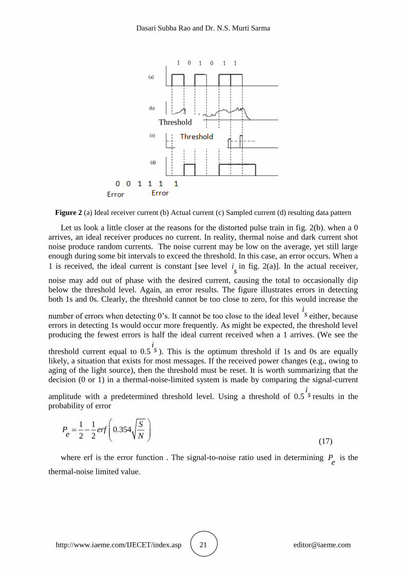
threshold is critical. Figure 2 illustrates how thermal noise produces detection errors. The

ideal (noise less) received current is shown in fig. 2 (a). It is followed by the actual current

[fig. 2(b)], showing the effects of added noise and filtering. This current is sampled near the

end of each bit interval (where the pulses are most likely to reach their maximum amplitudes)

with the result appearing in fig. 2 (c). At this point, the amplitude of each sample is compared

with a reference (or threshold) value. The threshold current is set somewhere between zero

and the ideal current expected when a 1 arrives ( is

in the figure). If the sample exceeds the

threshold, then it is further processed as a1. If the sample is lower than the threshold, it is

treated as 0. Fig. 2 (d) shows the resulting data pattern.



Figure 2 (a) Ideal receiver current (b) Actual current (c) Sampled current (d) resulting data pattern

Let us look a little closer at the reasons for the distorted pulse train in fig. 2(b). when a 0

arrives, an ideal receiver produces no current. In reality, thermal noise and dark current shot

noise produce random currents. The noise current may be low on the average, yet still large

enough during some bit intervals to exceed the threshold. In this case, an error occurs. When a

1 is received, the ideal current is constant [see level is

in fig. 2(a)]. In the actual receiver,

noise may add out of phase with the desired current, causing the total to occasionally dip

below the threshold level. Again, an error results. The figure illustrates errors in detecting

both 1s and 0s. Clearly, the threshold cannot be too close to zero, for this would increase the

number of errors when detecting 0‟s. It cannot be too close to the ideal level is either, because

errors in detecting 1s would occur more frequently. As might be expected, the threshold level

producing the fewest errors is half the ideal current received when a 1 arrives. (We see the

threshold current equal to 0.5is ). This is the optimum threshold if 1s and 0s are equally

likely, a situation that exists for most messages. If the received power changes (e.g., owing to

aging of the light source), then the threshold must be reset. It is worth summarizing that the

decision (0 or 1) in a thermal-noise-limited system is made by comparing the signal-current

amplitude with a predetermined threshold level. Using a threshold of 0.5is results in the

probability of error

1 10.354

2 2

SP erfe N

(17)

where erf is the error function . The signal-to-noise ratio used in determining Pe

is the

thermal-noise limited value.

Threshold



5. SIMULATION RESULT

Results with and without adaptive filter are shown in figs. 3- 15. Four types of plots based on

the observations are plotted. For every simulation one of the parameters, signal-to noise ratio

or the number of samples are varied and the resultant plots are observed.

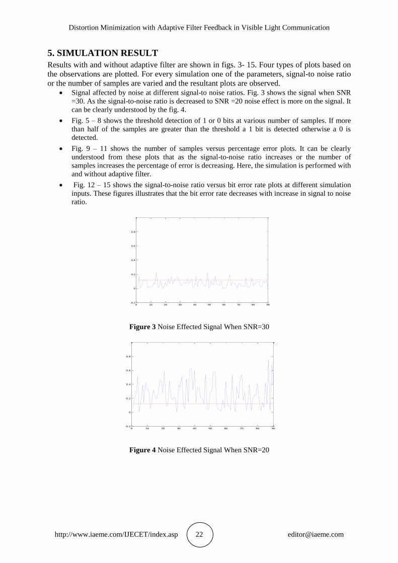
Signal affected by noise at different signal-to noise ratios. Fig. 3 shows the signal when SNR

=30. As the signal-to-noise ratio is decreased to SNR =20 noise effect is more on the signal. It

can be clearly understood by the fig. 4.

Fig. 5 – 8 shows the threshold detection of 1 or 0 bits at various number of samples. If more

than half of the samples are greater than the threshold a 1 bit is detected otherwise a 0 is

detected.

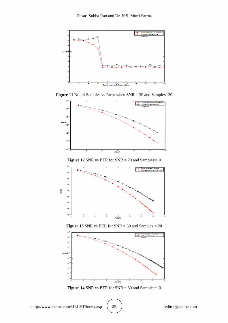
Fig. 9 – 11 shows the number of samples versus percentage error plots. It can be clearly

understood from these plots that as the signal-to-noise ratio increases or the number of

samples increases the percentage of error is decreasing. Here, the simulation is performed with

and without adaptive filter.

Fig. 12 – 15 shows the signal-to-noise ratio versus bit error rate plots at different simulation

inputs. These figures illustrates that the bit error rate decreases with increase in signal to noise

ratio.

Figure 3 Noise Effected Signal When SNR=30

Figure 4 Noise Effected Signal When SNR=20

0 10 20 30 40 50 60 70 80 90-0.2

0

0.2

0.4

0.6

0.8

0 10 20 30 40 50 60 70 80 90-0.2

0

0.2

0.4

0.6

0.8



Figure 5 Detection of bit 0 when No. of Samples = 5

Figure 6 Detection of bit 1 when No. of Samples =8


1 1.5 2 2.5 3 3.5 4 4.5 50

0.02

0.04

0.06

0.08

0.1

0.12

0.14

1 2 3 4 5 6 7 80

0.02

0.04

0.06

0.08

0.1

0.12

0.14

0.16

1 2 3 4 5 6 7 80

0.02

0.04

0.06

0.08

0.1

0.12




Figure 9 No. of Samples vs Error when SNR = 30 and Samples=10

Figure 10 No. of samples vs Error when SNR = 20 and Samples =10



Figure 11 No. of Samples vs Error when SNR = 30 and Samples=20

Figure 12 SNR vs BER for SNR = 20 and Samples=10

Figure 13 SNR vs BER for SNR = 30 and Samples = 20

Figure 14 SNR vs BER for SNR = 30 and Samples=10



6. CONCLUSIONS

This paper develop the approach of estimating signal based on Adaptive estimation is found

to be more accurate as compared to the thresholding method. From the observation it is found

that the % error fall down with the increase in samples considered for prediction using

Adaptive filtering. The Bit error rate Factor is also observed to be decreasing with the

increase in SNR and seen to be more accurate with Adaptive filtering than the thresholding

method. From all the above observations it could be concluded that Using Adaptive filter

optimum detection scheme we can reduce the probability of error (i.e., the bit error rate) and

by increasing the number of samples the percentage of error can also be decreased for a

optical fiber communication system.

REFERENCES

[1] Gerd Keiser, “Optical Fiber Communication”, McGraw-Hill International Editions.

[2] H.R.Burris, A.E.Reed, N.M.Namazi, M.J.Vilcheck, M.Ferraro, “Use of adaptive feedback

filtering in data detection in optical communication systems with multiplicative noise”,

Proceedings of IEEE , April 2001.

[3] John M. Senior, “Optical Fiber Communications Principles and Practice”, Second edition ,

Prentice Hall Publications.

[4] J.R.Barry and E.A.Lee, “Performance of coherent optical receivers”, Proceedings of

IEEE, Vol. 78, No. 8, August 1990.

[5] Joseph C. Palais, “Fiber Optic Communications”, Fourth edition, Pearson Education

Series, 2004.

[6] Nosu. K, “Advanced Coherent Lightwave Technologies”, IEEE Communications

Magazine, Vol.26, No.2 ,Feb. 1988.

[7] Datta D., “ Gangopadhyay R., Simulation studies on nonlinear bit synchronizers in APD-

based optical receivers”, IEEE Trans. On Communication, Vol.35, No.9, Sept. 1987, pp.

909-917.

[8] Stanley I.W., “ A tutorial review of techniques for coherent fiber transmission system”,

IEEE Communications Magazine, Vol.23, No.8, Aug. 1985.

[9] Dougherty, “Random processes for image and signal processing”.

[10] Estil V.Hoversten, Donald L.Snyder, Robert O.Harger, Koji Kurimoto, “Direct detection

optical communication receivers”, IEEE Trans. on Communications, Vol. com. 22, No.1,

Jan. 1974.

[11] P.T.Kalaivaani and A.Rajeswari , The Routing Algorithms For Wireless Sensor Networks

Through Correlation Based Medium Access Control For Better Energy Efficiency.

International Journal of Electronics and Communication Engineering and Technology

(IJECET), 3 (2) 2012,pp. 294–300.

[12] Renuka Bariker and Nagarathna K., Design and Development of Adaptive Routing

Algorithm to Reduce Distortion during Video Transmission, International Journal of

Electronics and Communication Engineering & Technology , 7(4), 2016, pp. 01–12.



AUTHOR’S PROFILE

Dasari Subba Rao is a research Scholar from Rayalaseema University and

working as Associate Professor Professor of ECE in Siddartha Institute of

Engineering and Technology. He has done his Graduation in Engineering

(ECE) in 2003 from JNTU, Hyderabad and Post Graduation in 2007 with

specialization in Embedded Systems from SRM University, Chennai. He

published 26 papers in International Journal, He is the life time member of

ISTE. His area of interest is Wireless Communications.

Dr.N.S.Murti Sarma belongs to K. Pedapudi , East Godavary district of

Andhra Pradesh state, India2. He received his Model Diploma for

Technicians(MDT), offered with collaboration of United Sates of Soviet

Russia (USSR), with specialization in production of radio apparatus (RA)

from Government Polytechnic of Masabtank, Hyderabad, his B.Tech from

Jawharlal Nehru Technological University (JNTU) College of Engineering,

Hyderabad in 1990, his M.E with specialization in Microwaves and Radar

Engineering(MRE) from Osmania University in 1996 and his Ph.D in E.C.E

from O.U, Hyderabad in 2002. As a Part of his diploma curriculum, He was at

nuclear instruments division of instruments group in Electronics corporation

of India limited (ECIL), Hyderabad as technician apprentice in 1984.

From 1991 to 1996 he was a lecturer to U.G courses in electronics,

physics in faculty of science and various subjects of electronics and

communications engineering for diploma holders (FDH) program of JNTU

Engineering College at Hyderabad, and from 1996 to 2001 he was with R&T

Unit for navigational electronics (NERTU). During his association with

NERTU, he executed projects sponsored by RCA, VSSC, DLRL and DST.

His research interests include electromagnetic modeling, atmospheric studies,

optical fiber communication, low power VLSI, signal processing. Several

international and national publications are under his credit.

He continued his teaching from 2001 and currently at Sreenidhi

Institute of Science and Technology as a professor of ECE . As one of the

earlier assignments now he was Principal of SV Insititute of Technology and

Engineering (SVIET) and professor of electroncs and communications

Engineering of SV group of institutions. He teaching interests for

undergraduate courses includes Electromagnetic theory, antennas and

propagation and microwave engineering, post graduate courses in

communication systems and microwave radar engineering. Dr. N.S.Murthy

Sarma is life member of Institute of Science and Technology education

(ISTE) since 2002 and fellow of institute of electronics and

telecommunication engineers (IETE) since 2003, fellow of Institution of

Engineers IE(I) and Member of Institute of Electrical and Electronics

Engineers (IEEE) since 2010. He usually reviewers papers for international

journals viz. international journal of computer science and Engineering

systems and international journal of International Journal of Emerging

Technologies and Applications in Engineering Technology and Sciences ,

besides a regular conference reviewer of conferences(since 2010) of IEEE

with immediate recent assignment of ADVCIT'2014. . He is one of the

recognized Ph.D Supervisors of engineering faculty, Around Eight research

scholars are working with him under Ph.D. programme of

JNTUH/JNTUK/KLU in the area of Communications, Low power VLSI,

GPS/GLONASS, since 2008.

Date post:	30-May-2020
Category:	Documents
Upload:	others
View:	24 times
Download:	0 times

DISTORTION MINIMIZATION WITH ADAPTIVE FILTER FEEDBACK … · 2017-11-10 · Distortion Minimization...

Documents