Biometrika (2008), 95, 1, pp. 17–33 doi: 10.1093/biomet/asm092 Advance Access publication 4 February 2008 C 2008 Biometrika Trust Printed in Great Britain Distortion of effects caused by indirect confounding BY NANNY WERMUTH Department of Mathematical Statistics, Chalmers/G ¨ oteborgs Universitet, Gothenburg, Sweden [email protected]AND D. R. COX Nuffield College, Oxford OX1 1NF, U.K. david.cox@nuffield.ox.ac.uk SUMMARY Undetected confounding may severely distort the effect of an explanatory variable on a response variable, as defined by a stepwise data-generating process. The best known type of distortion, which we call direct confounding, arises from an unobserved explanatory variable common to a response and its main explanatory variable of interest. It is relevant mainly for observational studies, since it is avoided by successful randomization. By contrast, indirect confounding, which we identify in this paper, is an issue also for intervention studies. For general stepwise-generating processes, we provide matrix and graphical criteria to decide which types of distortion may be present, when they are absent and how they are avoided. We then turn to linear systems without other types of distortion, but with indirect confounding. For such systems, the magnitude of distortion in a least-squares regression coefficient is derived and shown to be estimable, so that it becomes possible to recover the effect of the generating process from the distorted coefficient. Some key words: Graphical Markov model; Identification; Independence graph; Linear least-squares regression; Parameter equivalence; Recursive regression graph; Structural equation model; Triangular system. 1. INTRODUCTION In the study of multivariate dependences as representations of a potential data-generating pro- cess, important dependences may appear distorted if common explanatory variables are omitted from the analysis, either inadvertently or because the variables are unobserved. This is an instance of the rather general term confounding. There are, however, several distinct sources of distortion when a dependence is investigated within a reduced set of variables. The different ways in which such distortions arise need clari- fication. We do this by first giving examples using small recursive linear systems for which the generating process has a largely self-explanatory graphical representation. Later, these ideas are put in a general setting. 2. SOME INTRODUCTORY EXAMPLES 2·1. Direct confounding The most common case of confounding arises when an omitted background variable is both explanatory to a response of primary interest and also to one of its directly explanatory variables.
Undetected confounding may severely distort the effect of an explanatory variable on a responsevariable, as defined by a stepwise data-generating process. The best known type of distortion,which we call direct confounding, arises from an unobserved explanatory variable common toa response and its main explanatory variable of interest. It is relevant mainly for observationalstudies, since it is avoided by successful randomization. By contrast, indirect confounding, whichwe identify in this paper, is an issue also for intervention studies. For general stepwise-generatingprocesses, we provide matrix and graphical criteria to decide which types of distortion may bepresent, when they are absent and how they are avoided. We then turn to linear systems withoutother types of distortion, but with indirect confounding. For such systems, the magnitude ofdistortion in a least-squares regression coefficient is derived and shown to be estimable, so that itbecomes possible to recover the effect of the generating process from the distorted coefficient.
In the study of multivariate dependences as representations of a potential data-generating pro-cess, important dependences may appear distorted if common explanatory variables are omittedfrom the analysis, either inadvertently or because the variables are unobserved. This is an instanceof the rather general term confounding.
There are, however, several distinct sources of distortion when a dependence is investigatedwithin a reduced set of variables. The different ways in which such distortions arise need clari-fication. We do this by first giving examples using small recursive linear systems for which thegenerating process has a largely self-explanatory graphical representation. Later, these ideas areput in a general setting.
2. SOME INTRODUCTORY EXAMPLES
2·1. Direct confounding
The most common case of confounding arises when an omitted background variable is bothexplanatory to a response of primary interest and also to one of its directly explanatory variables.
18 NANNY WERMUTH AND D. R. COX
Fig. 1. Simple example of direct confounding. (a) Y1 de-pendent on both Y2 and U ; Y2 dependent on U and U to beomitted. In a linear system for standardized variables, theoverall dependence of Y1 on Y2 is α + δγ , with confound-ing effect δγ due to the unobserved path from Y1 to Y2 viaU . (b) Graph derived from Fig. 1(a) after omitting U . Adashed line added to 1≺ 2 for the induced association.
Generating dependence α preserved, but not estimable.
In Fig. 1(a), which shows this simplest instance, the directions of the edges indicate that U is tobe regarded as explanatory to both the response Y1 and to Y2; Y2 is, in addition, explanatory toY1. We suppose here for simplicity that the random variables have marginally zero means andunit variances.
The generating process is given by three linear equations,
Y1 = αY2 + δU + ε1, Y2 = γU + ε2, U = ε3, (1)
where each residual, εi , has mean zero and is uncorrelated with the explanatory variables on theright-hand side of an equation.
If, as is indicated by the crossed out node in Fig. 1(a), U is marginalized over, the conditionaldependence of Y1 on only Y2 is obtained, which consists of the generating dependence α andan effect of the indirect dependence of Y1 on Y2 via U . This may be seen by direct calculation,assuming that the residuals εi have a Gaussian distribution, from
E (Y1 | Y2, U ) = αY2 + δU, E (Y2 | U ) = γU, E (U ) = 0,
leading to
E (Y1 | Y2) = αY2 + δ E (U | Y2) = {α + δγ var(U )/var(Y2)} Y2 = (α + δγ )Y2· (2)
Thus, the generating dependence α is distorted in the conditional dependence of Y1 on Y2 alone,unless δ = 0 or γ = 0. However, this would have been represented by a simpler generatingprocess, in which a missing arrow for (1, U ) indicates δ = 0 and a missing arrow for (2, U )shows γ = 0. Marginal independence of Y2 and U (γ = 0) can be achieved by study design. It issatisfied if Y2 represents a treatment variable and randomization is used successfully to allocateindividuals to treatments. In that case, all direct dependences affecting the treatment variable Y2
are removed from the generating process, including those of unobserved variables. Effects of thelack of an association between Y2 and U are explored for more general relationships by Cox &Wermuth (2003) and by Ma et al. (2006). In general, the dependence of Y1 on U, given Y2, mayvary with the levels y2 of Y2.
Conditions under which a generating coefficient α remains unchanged follow also from therecursive relation of linear least-squares regression coefficients (Cochran, 1938), namely
β1 | 2 = β1 | 2·3 + β1 | 3·2β3 | 2, (3)
where we use a slight modification of Yule’s notation for partial regression coefficients. Forexample, β1 | 2·3 is the coefficient of Y2 in linear least-squares regression of Y1 on both Y2 and Y3,
Distortion of effects 19
and we note for Fig. 1 that α = β1 | 2·3 and δ = β1 | 3·2. Cochran’s result (3) uses implicitly linearexpectations to obtain β3 | 2. As we shall explain later, these linear expectations are well definedfor recursive linear least-squares equations, such as (1), which have uncorrelated residuals, butwhich do not necessarily have Gaussian distributions.
For the later general discussion, we also need a graphical representation of the structureremaining among the observed variables, here of Y1 and Y2, as given in Fig. 1(b). The commondependence on U induces an undirected association between the two observed variables, shownby a dashed line. A dashed line represents an association that could have been generated by asingle common unobserved explanatory variable. From the generating equations (1), we obtainlinear equations with correlated residuals,
Y1 = αY2 + η1, Y2 = η2, (4)where
η1 = δU + ε1, η2 = γU + ε2.
This shows directly that α cannot be estimated from the three elements of the covariance matrixof (Y1, Y2), since the three non-vanishing elements of the residual covariance matrix and α
give four parameters for the equations (4). As a consequence, the generating dependence,α, also cannot be recovered from the conditional dependence of Y1 on Y2 alone, given byβ1 | 2 = α + δγ .
When the dependence represented by generating coefficient α is not estimable as in the inducedequations (4), the equations are said to be under-identified. In systems larger than the one inFig. 1(b), it may be possible to recover the generating dependence from the observed variables,provided there are so-called instrumental variables; for the extensive econometric literature,which builds on early work by Sargan (1958), see Hausmann (1983) or Angrist & Krueger(2001).
As we shall see, direct confounding of a generating dependence of variable pair Yi , Y j , say, isabsent, in general, if there is no double edge, i≺ j , induced in the derived graph.
2·2. Two avoidable types of distortion
We describe next two further types of distortion that can typically be avoided if the generatingprocess is known and the distortions involve observed variables. One is under-conditioning. Itarises by omitting from an analysis those variables that are intermediate between the explanatoryvariable and an outcome of primary interest. The other is over-conditioning. It arises by using asan explanatory variable to the outcome of primary interest, a variable which is, in fact, itself aresponse of this outcome.
We give two simple examples in Fig. 2, again for standardized variables that are linearly related.The boxed-in node, �◦ , indicates conditioning on given levels of a variable, and a crossed outnode, � �◦, means, as before, marginalizing.
In Fig. 2(a), with Y3 representing a treatment variable, interest could often be in what is calledthe total effect of Y3 on Y1. Then, marginalizing over the intermediate variable Y2 is appropriateand β1 | 3 = δ + αγ is estimated. Suppose, however, that the generating dependence of responseY1 on Y3 , given Y2 is of main interest; then the direct effect δ in the data-generating process isto be estimated, and a decomposition of the total effect β1 | 3 becomes essential, into the directeffect, δ, and the indirect effect, αγ , via the intermediate variable Y2. In this case, omission of Y2
would be an instance of under-conditioning, leading to a mistaken interpretation; for example,see Wermuth & Cox (1998b).
20 NANNY WERMUTH AND D. R. COX
Fig. 2. Distortions due to under- and over-conditioning. (a)Generating dependence β1 | 3·2 = δ distorted with β1 | 3, i.e. af-ter removing Y2 from conditioning set of Y1 ; (b) Generatingdependence β2 | 3 = γ distorted with β2 | 3·1, i.e. after including
Y1 into the conditioning set of Y2.
For Fig. 2(b), the following form of the recursive relation of least-squares regression coefficientsβ2 | 3·1 = β2 | 3 − β2 | 1·3β1 | 3 gives, together with β2 | 1·3 = β1 | 2·3σ22 | 3/σ11 | 3,
β2 | 3·1 = γ − {(1 − γ 2)/
(1 − ρ2
13
)}αρ13, with ρ13 = δ + αγ .
The generating dependence could not be recovered if no information were available for Y2 inFig. 2(a) or for Y1 in Fig. 2(b).
More complex forms of over-conditioning result by both marginalizing and conditioning. Thesimplest more general form is the presence of the following path:
i ��◦ ≺ � �◦ ��◦ ≺ j .
With any type of over-conditioning, the roles given by the generating process are interchanged forsome variables, since a response to an outcome variable becomes included in the conditioning setof this outcome. Presence of strong distortions due to over-conditioning typically leads directlyto a mistaken interpretation.
As we have seen, consequences of under- and over-conditioning can be quite different. However,after a set of variables is omitted from the generating process, both over- and under-conditioningfor a response are avoided by the same strategy: by considering the conditional dependence onall and only those of the observed variables that are explanatory for response, either directly orindirectly via intermediate variables.
In the following two examples of indirect confounding, there is no direct confounding andthere is no distortion due to over- or to under-conditioning.
2·3. Indirect confounding in an intervention study
A simple system without direct confounding, but with distortions of the generating dependenceof Y on Tp, is shown in Fig. 3.
It concerns an intervention study and is adapted from Robins & Wasserman (1997), whoshowed that the generating dependence of the main outcome variable, Y , on past treatment, Tp,given both the more recent treatment, Tr, and the unobserved health status, U , of a patient, cannotbe estimated consistently by any least-squares regression coefficient in the observed variables, inspite of the use of randomization when administering the two treatments sequentially.
A past treatment Tp is decoupled from U due to full randomized allocation of treatments toindividuals, and there is an intermediate binary outcome, A. The recent treatment, Tr, is decoupledfrom both Tp and U , but not from A, since randomized allocation of treatments to individuals isat this stage, assumed to be conditional on the level of the intermediate outcome variable A.
For some detailed discussion of the structure represented by the graph in Fig. 3, we turn nowto a linear system of standardized variables in which observed variables (1, 2, 3, 4) correspond to
Distortion of effects 21
Fig. 3. Generating process in five variables, missing edge for (Tp, U ) dueto full randomized allocation of individuals to treatments, and missingedges for (Tr, U ) and (Tr, Tp) due to randomization conditionally, givenA. With U unobserved, no direct confounding results, but the generatingdependence of Y on Tp (but not of Y on Tr) becomes indirectly confounded.
(Y, Tr, A, Tp) and obtain the equations with uncorrelated residuals, defined implicitly by Fig. 4(a),as
From Fig. 4(a), the graph for the remaining four observed variables in Fig. 4(b) is derived byreplacing the path 1≺ U �3 by a dashed line for (1,3).
Fig. 4. (a) The graph of Fig. 3 for a linear system in standardized variables and (b) the derived graphwith an induced association for (1,3), shown as a dashed line; no direct confounding of α, the generatingdependence of 1 on 4, but the confounding path, 1 3≺ 4, turns β1 | 4·23 into a distorted measure of
α = β1 | 4·3U .
The correlation matrix of the observed variables is, by direct computation or by tracing paths,i.e. by repeated use of recursive relations for least-squares coefficients,
corr(Y1, Y2, Y3, Y4) =
⎛⎜⎜⎝
1 λ + αθν + δγ ν λν + αθ + δγ α + λνθ
· 1 ν νθ
· · 1 θ
· · · 1
⎞⎟⎟⎠ ,
where the dots indicate entries in a symmetric matrix, left out as redundant.Furthermore, each of the four possible least-squares coefficients of Y1, regressed on Y4 and on
some or none of Y2 and Y3, is a distorted measure of the generating dependence α, since
β1 | 4 = α + λνθ, β1 | 4·2 = α − ν2θδγ /(1 − ν2θ2), β1 | 4·23 = β1 | 4·3 = α − θδγ /(1 − θ2)·This verifies the result of Robins & Wasserman (1997) for a purely linear system and explainshow effect reversal can occur, depending on the signs and relative magnitudes of the two termsin these last formulae. The distortion of α in β1 | 4·23, which is due to what we call indirect
22 NANNY WERMUTH AND D. R. COX
confounding, results by the combination of conditioning on Y3, which is indirectly explanatoryfor the response Y1, and of marginalizing over U , which is a common explanatory variable forboth Y1 and Y3.
The explicit expressions for the least-squares coefficients show, in addition, that the generatingcoefficient α may, in this case, be recovered from the observed variables, for instance, withβ2 | 4 = νθ and β1 | 2·34 = λ; the same holds for least-squares estimates, so that the generatingcoefficient α is identifiable for the given process, see § 6·2.
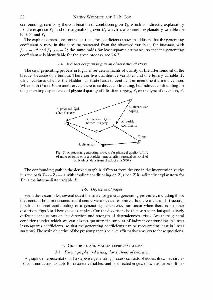
2·4. Indirect confounding in an observational study
The data-generating process in Fig. 5 is for determinants of quality of life after removal of thebladder because of a tumour. There are five quantitative variables and one binary variable A,
which captures whether the bladder substitute leads to continent or incontinent urine diversion.When both U and V are unobserved, there is no direct confounding, but indirect confounding forthe generating dependence of physical quality of life after surgery, Y , on the type of diversion, A.
Fig. 5. A potential generating process for physical quality of lifeof male patients with a bladder tumour, after surgical removal of
the bladder; data from Hardt et al. (2004).
The confounding path in the derived graph is different from the one in the intervention study:it is the path Y Z A with implicit conditioning on Z , since Z is indirectly explanatory forY via the intermediate variable X .
2·5. Objective of paper
From these examples, several questions arise for general generating processes, including thosethat contain both continuous and discrete variables as responses. Is there a class of structuresin which indirect confounding of a generating dependence can occur when there is no otherdistortion, Figs 3 to 5 being just examples? Can the distortions be then so severe that qualitativelydifferent conclusions on the direction and strength of dependencies arise? Are there generalconditions under which we can always quantify the amount of indirect confounding in linearleast-squares coefficients, so that the generating coefficients can be recovered at least in linearsystems? The main objective of the present paper is to give affirmative answers to these questions.
3. GRAPHICAL AND MATRIX REPRESENTATIONS
3·1. Parent graphs and triangular systems of densities
A graphical representation of a stepwise generating process consists of nodes, drawn as circlesfor continuous and as dots for discrete variables, and of directed edges, drawn as arrows. It has
Distortion of effects 23
an ordered node set V = (1, 2, . . . , d), such that a component variable Yi of a vector variable YV
corresponds to node i and, for i < j , the relationship between variables Yi and Y j is interpretedwith Y j being potentially explanatory to response Yi .
For each node i , there is a subset par(i) of r (i) = (i + 1, . . . , d), called the parent set of i , withthe corresponding variables said to be directly explanatory for Yi . An i j-arrow starts at node jand points to node i, if and only if node j is a parent of node i ; the graph, denoted by GV
par, isnamed the parent graph.
A joint density fV , written compactly in terms of nodes and of the form
fV =d∏
i=1
fi | par (i), (6)
is then generated over the given parent graph by starting with the last background variable, Yd ,continuing with Yd−1, up to Y1, the response of primary interest. In that way, the independencestructure is fully described by the parent graph: if the i j-arrow, i.e. the edge for node pair (i, j),is missing, then Yi is independent of Y j , given Ypar (i), written in terms of nodes as i ⊥⊥ j | par (i).If the i j-arrow is present, then Yi is dependent on Y j , given Ypar (i)\ j .
For the later results, some further definitions for graphs are useful. An i j-path is a sequence ofedges which join the path endpoint nodes i and j via distinct nodes. Nodes along a path, called itsinner nodes, exclude the path endpoints. An edge is regarded as a path without inner nodes. Foran i j-path which starts with an arrow-end at node j , meets an arrow-end at each inner node andends with an arrow-head at i , node j is called an ancestor of i and the set of ancestors is denotedby anc(i). Variables attached to such inner nodes are intermediate between Yi and Y j . A node j ,which is an ancestor but not a parent of i , indicates that Y j is only indirectly explanatory for Yi .
3·2. Linear triangular systems
Instead of a joint density, a linear triangular system of equations may be generated over a givenparent graph. Then, for mean-centred variables, the linear conditional expectation of Yi on Yr (i),where as before r (i) = (i + 1, . . . d), is
E lin(Yi | Yr (i)) = �i | par(i)Ypar(i), (7)
if the residuals, denoted by εi , are uncorrelated with Y j for all j in r (i) (Cramer, 1946, p. 302)and if there is a direct contribution to linear prediction of Yi only for j, a parent node of i . Thus,E lin is to be interpreted as forming a linear least-squares regression and �i | par(i) denotes a rowvector of nonzero linear least-squares regression coefficients.
A missing i j-arrow means, in this case, that Yi is linearly independent of Y j , given Ypar(i), andthis is reflected in βi | j ·par(i) = 0. The linear equations, corresponding to (7), are in matrix form
AY = ε, (8)
where A is an upper-triangular matrix with unit diagonal elements, and ε is a vector of zero-mean, uncorrelated random variables, called residuals. The diagonal form of the positive definiteresidual covariance matrix, cov(ε) = , defines linear least-squares regression equations, suchthat the nonzero off-diagonal elements Ai j of A are
The concentration matrix implied by (8) is �−1 = AT −1 A. The matrix pair (A, −1) is alsocalled a triangular decomposition of �−1. It is unique for the fixed order given by V . For a given�−1 of dimension d, there are d! possible triangular decompositions, so that linear least-squares
24 NANNY WERMUTH AND D. R. COX
coefficients βi | j ·C are defined for any subset C of V without nodes i and j . Thus, for the examplesset out in § 2, Gaussian distributions of the residuals are not needed; the same results are achievedfor linear triangular systems (8) which have uncorrelated residuals.
3·3. Edge matrices and structural zeros
The binary matrix representation of the parent graph of a linear triangular system isA = In[A],where the indicator operator In replaces every nonzero element in a matrix by a one. It is calledan edge matrix, since off-diagonal ones represent edges present in the graph. The edge matrix ofGV
par of a joint density (6) is the d × d upper triangular binary matrix with elementsAi j defined by
Ai j ={
1 if and only if i ≺ j in GVpar or i = j,
0 otherwise.(10)
It is the transpose of the usual adjacency matrix representation of the graph with additional onesalong the diagonal to simplify transformations, such as marginalizing.
New edge matrices are induced after changing conditioning sets of dependencies, as given bythe parent graph. For each i j-one in an induced-edge matrix, at least one i j-path can be identifiedin the given parent graph that leads in the family of linear systems generated over the parent graphto a nonvanishing parameter for pair (Yi , Y j ); see, for example, § 3 of Wermuth & Cox (1998a).Whenever no such path exists, an i j-zero is retained in the induced-edge matrix. It indicates forthe linear system that the corresponding parameter is structurally zero, i.e. that it remains zeroas a consequence of the generating process. Therefore, we denote edge matrices by calligraphicletters that correspond to the latin letters of the associated parameter matrices in linear systems.
4. SOME PRELIMINARY RESULTS
4·1. Some early results on triangular systems
Linear triangular systems (7) have been introduced as path analyses in genetics (Wright, 1923,1934) and as linear recursive equations with uncorrelated residuals in econometrics (Wold, 1954).Early studies of their properties include Tukey (1954), Wermuth (1980) and Kiiveri et al. (1984).They form a subclass of linear structural equations (Goldberger, 1991, Ch. 33, p. 362)
Linear triangular systems (7) and triangular systems of densities (6) are both well suited todescribe development without and with interventions. Both form a subclass of graphical Markovmodels (Cox & Wermuth, 1993, 1996; Wermuth, 2005). For graphical models based on a specialtype of distributional assumption, namely the conditional Gaussian distribution, see Edwards(2000), Lauritzen (1996) and Lauritzen & Wermuth (1989).
4·2. Omitting variables from a triangular system
For a split of YV into any two component variables YM and YN with N = V \ M , the densityfV in (6) can be factorized in the form
fV = fM | N fN .
One may integrate over YM to obtain the structure in the joint marginal density fN of YN , impliedby the generating process.
Essential aspects of this structure are captured by the changes resulting for the parent graph. Wedenote by V = (M, N ) the correspondingly ordered node set and by G N
rec, the graph of recursivedependencies derived for the reduced node set N , where the order of nodes within N is preservedfrom V . The objective is to deduce the independence structure of G N
rec from that of the parentgraph and to define different types of association introduced by marginalizing over YM .
Distortion of effects 25
4·3. Two matrix operators
To set out changes in edge matrices, we start with a general type of edge matrix F , such asfor A, �−1 and �, denote the associated linear parameter matrix by F , and apply two matrixoperators, called partial closure and partial inversion.
Let F be a square matrix of dimension d with principal submatrices that are all invertible andlet a be any subset of V . Let, further, b = V \ a and let an associated binary edge matrix F bepartitioned according to (a, b). We also partition F and B accordingly and denote by Bab thesubmatrix of B with rows pertaining to node components a and columns to components b. Thenthe operator, called partial inversion, transforms F into inva F and the operator, called partialclosure, transforms F into the associated edge matrix zeraF . They are defined as follows.
DEFINITION 1 (Partial inversion and partial closure; Wermuth et al., 2006b). The operators ofpartial inversion and partial closure are
inva F =(
F−1aa −F−1
aa Fab
Fba F−1aa Fbb − Fba F−1
aa Fab
), zeraF = In
[( F−aa F−
aaFab
FbaF−aa Fbb + FbaF−
aaFab,
)],
where
F−aa = In[(k Iaa − Faa)−1], (11)
with k − 1 denoting the dimension of Faa and I an identity matrix.
Adding a sufficiently large constant along the diagonal in (11) ensures that an invertible matrixis obtained, that the inverted matrix has nonnegative elements and that this inverse has a zeroentry, if and only if there is a structural zero in F−1. If Faa = Aaa is upper-triangular, then ani j-one is generated in A−
aa , if and only if j is an ancestor of i in the graph with edge matrix Aaa .If instead Faa is symmetric, an i j-one is generated in F−
aa if and only if there is an i j-path in thegraph with edge matrix Faa .
Both operators can be applied to a sequence of distinct subsets of a in any order to give inva Fand zeraF . Closing paths repeatedly has no effect, but partial inversion is undone by applying itrepeatedly, i.e. inva(inva F) = F . Another important property of partial inversion is that
F(
ya
yb
)=
(za
zb
)implies inva F
(za
yb
)=
(ya
zb
)· (12)
Repeated application of these two operators will be used here to identify relevant propertiesof triangular systems. In essence, partial inversion isolates the random variable of interest aftermarginalization and partial closure specifies the implied graphical structure.
4·4. The induced recursive regression graph
For a linear triangular system, AY = ε in (7), with diagonal covariance matrix of the residualsε and a parent graph with edge matrix A, let M denote any subset of V to be marginalized over, letN = V \ M and let A, A be the matrices A,A arranged and partitioned according to V = (M, N )and preserving within subsets the same order as in V . Then we define
B = invM A, B = zerMA, (13)
to obtain the induced equations in terms of and B, and the graph in terms of B. After applyingproperty (12) to AY = ε, we have that
invM A(
εM
YN
)=
(YM
εN
)·
26 NANNY WERMUTH AND D. R. COX
The bottom row of this equation gives the observed variables YN that remain after marginalizingover YM as a function of components of ε and B. We summarize this in Lemma 1.
LEMMA 1 (The induced recursive regression graph. Wermuth & Cox, 2004; Corollary 1 andTheorem 3). The recursive equations in YN obtained from a linear triangular system (7), whichare orthogonal to the equations in YM corrected for linear least-squares regression on YN , haveequation parameters defined by BN N and residual covariances defined by KN N = cov(ηN ). Theinduced recursive regressions equations are
BN N YN = ηN , ηN = εN − BN MεM , KN N = N N + BN M M M BTN M . (14)
The edge matrix components of the recursive regression graph G Nrec , induced by triangular
systems (6) or (7) after marginalizing over YM , are
KN N , KN N = In[IN N + BN MBT
N M
]. (15)
The key issue here is that the edge matrix components of G Nrec derive exclusively from special
types of path in G Npar, represented by A, and, since probabilistic independence statements defined
by a parent graph combine in the same way as linear independencies specified by the same graph,the edge matrix induced by the linear system holds for all densities generated over the same GV
par;see Marchetti and Wermuth (2008).
In general, edge matrices indicate both edges present in a graph, by i j-ones, and structurallyzero parameters in a linear system, by i j-zeros. The types of induced edge are specified by usingthe following convention.
DEFINITION 2 (Types of edge represented by a matrix). An i j-one in F , an edge matrix derivedfrom A for an induced linear parameter matrix F, represents
(i) an arrow, i ≺ j , if F is an equation parameter matrix,(ii) an i j-dashed line, i j , if F is a residual covariance matrix.
Thus, for instance, i j-arrows result with BN N and i j-dashed lines with KN N . The type ofinduced edge relates more generally to the defining matrix products.
DEFINITION 3 (Types of edge resulting by edge matrix products). Let an edge matrix productdefine an association-inducing path for a family of linear systems. Then the generated edgeinherits the edge ends of the left-hand and of the right-hand matrix in the product.
Thus, AN MA−M MAM N results in arrows and BN MBT
N M leads to dashed lines as a condensednotation for generating paths which have arrow-heads at both path endpoints.
4·5. Linear parameter matrices and induced-edge matrices
For the change, for instance, from parameter matrices BN N , KN N in the linear systems (14)to induced-edge matrix components BN N ,KN N in (15), one wants to ensure that every matrixproduct and every sum of matrix products has nonnegative elements, so that no additional zerois created and possibly, all zeros are retained. This is summarized as follows.
LEMMA 2 (Transforming parameter matrices in linear systems into edge matrices). Letinduced parameter matrices be defined by parameter components of a linear system FY = ζ ,with correlated residuals, such that the matrix products hide no self-cancellation of an operation,such as a matrix multiplied by its inverse. Let, further, the structural zeros of F be given by F .Then the induced-edge matrix components are obtained by replacing, in the defining equations,
(i) every inverse matrix, F−1aa say, by the binary matrix of its structural zeros F−
aa,(ii) every diagonal matrix by an identity matrix of the same dimension,
Distortion of effects 27
(iii) every other submatrix, −Fab or Fab say, by the binary submatrix of structural zeros, Fab,(iv) and then applying the indicator function.
Thus, for instance, BN N = In[AN N + AN MA−M MAM N ] may be obtained in this way from
BN N = AN N − AN M A−1M M AM N .
The more detailed results that follow are obtained by starting with equations (14) for theobserved vector variable YN , applying the two matrix operators, the above stated types of trans-formation and by orthogonalizing correlated residuals. The last task is achieved for an arbitrarysubset a of V and b = V \ a, after transforming ηb into residuals corrected for marginalizationover Ya , i.e. by taking ηb−a = ηb − Cbaηa , and then by conditioning ηa on ηb−a , i.e. by obtain-ing ηa | b−a = ηa − cov(ηa, ηb−a){cov(ηb−a)}−1ηb−a . For this, one uses the appropriate residualcovariance matrix partially inverted with respect to b.
4·6. Consequences of the induced recursive regression graph
In Lemma 1, we have specified the structure for YN , obtained after marginalizing over YM . Tostudy YN in more detail, let a be any subset of N and b = N \ a. Let, further, �a | b be the matrixof regression coefficients obtained by linear least-squares regression of Ya on Yb. An element�a | b for i of a and j of b is the least-squares regression coefficient βi | j ·b\ j . The edge matrixcorresponding to �a | b is denoted by Pa | b , with element Pi | j ·b\ j .
Suppose now that the parameter matrices of linear recursive equations (14) and correspondingedge matrices (15) are arranged and partitioned according to N = (a, b) and that, within subsets,the order of nodes remains as in N . Then we define
CN N = inva BN N , CN N = zera BN N , (16)
and, with WN N = cov(ηa, ηb − Cbaηa) and WN N the corresponding induced-edge matrix,
QN N = invb WN N , QN N = zerb WN N , (17)
to obtain with Pa | b the independence statements induced by G Nrec for Ya , given Yb.
LEMMA 3 (The induced-edge matrix of conditional dependence of Ya on Yb; Wermuth &Cox, 2004, Theorem 1). The linear least-squares regression coefficient matrix �a | b induced bya system of linear recursive regression (14) in G N
rec is
�a | b = Cab + Caa QabCbb, (18)
and the edge matrix Pa | b induced by a recursive regression graph G Nrec is
Pa | b = In[Cab + CaaQabCbb]. (19)
The independence interpretation of recursive regression graphs results from Lemma 3, if a issplit further into any two nonempty subsets α and d and b into two nonempty subsets β and c. Forthe dependence of Yα on Yβ , given Yc, i.e. for a conditional dependence in the marginal densityfαβC , one obtains the induced-edge matrix Pα | β·c as a submatrix of Pa | b:
Pa | b =(Pα | β·c Pα | c·βPd | β·c Pd | c·β
).
COROLLARY 1 (Independence induced by a recursive regression graph). The following state-ments are equivalent consequences of the induced recursive regression graph G N
rec :(i) Pα | β·c = 0;
(ii) α ⊥⊥ β | c is implied for all triangular systems of densities generated over a parent graph;(iii) In[Cαβ + CαaQabCbβ] = 0.
28 NANNY WERMUTH AND D. R. COX
It follows further from (19) that the conditional dependence of Yi on Y j , given Yb\ j coincideswith the generating dependence corresponding toAi j = 1, if CiaQabCbj = 0 andAimA−
mmAmj =0, where m = M ∪ a. The first condition means absence of an i j-path in G N
rec via inducedassociations captured by Qab. The second condition means that, in GV
par, node j is not an ancestorof i, such that all inner nodes of the path are in m. With appropriate choices of i and b, thedistortions described in the examples of § 2 are obtainable by using (18).
However, to correct for the distortions, one needs to know when the parameters induced forG N
rec are estimable. From the discussion in § 2·2, this is not possible, in general. We therefore turnnext to systems without over- and under-conditioning concerning components of YN .
5. DISTORTION IN THE ABSENCE OF OVER- AND UNDER-CONDITIONING
For any conditional dependence of Yi on Yb, we let b coincide with the observed ancestors ofnode i , i.e. we take b = anc(i) ∩ N and node i in a = N \ b. The corresponding modification ofLemma 3 results after observing that, in this case, there is no path from d = a \ i to node i, sothat (invd BN N )S,S = BSS with S = N \ d and that, in addition, Cba = Bba = 0.
PROPOSITION 1 (The conditional dependence of Yi on Yb in the absence of over- and under-conditioning). The graph G N
rec, obtained after marginalizing over variables YM induces thefollowing edge vector for the conditional dependence of Yi on Yb:
Pi | b = In[Bib + (KibK−bb)Bbb]. (20)
In addition, the linear system to G Nrec induces the following vector of least-squares regression
coefficients:
�i | b = Bb + (Kib K −1bb )Bbb· (21)
The conditional dependence of Yi on Y j , given Yb\ j , measures the generating dependence corre-sponding to Ai j = 1 without distortions
(i) due to unobserved intermediate variables if Ai MA−M MAM j = 0, and
(ii) due to direct confounding if Ki j = 0, and(iii) due to indirect confounding if (KibK−
bb)Bbj = 0.
Distortions of type (i) are avoided if the observed node set N consists of the first dN nodesof V = (1, . . . , d). Then no path can lead from a node in N to an omitted node in M, so thatAN M = 0 and hence BN N = AN N , BN N = AN N .
COROLLARY 1 (Paths of indirect confounding in the absence of over- and under-conditioning).In a graph G N
rec, only the following two types of path may introduce distortions due to indirectconfounding:
(i) (KabK−bb)i j � 0,
(ii) (KibK−bb)Bbj � 0.
When three dots indicate that there may be more edges of the same type, coupling more distinctnodes, then typical paths of type (i) and (ii) are, respectively,
i �◦ . . . �◦ �◦ j, i �◦ . . . �◦ �◦ ≺ j,
where each node �◦ along the path is conditioned on and represents a node which is a forefatherof node i , i.e. an ancestor but not a parent of i . In Fig. 4(b), the confounding path 1 3≺ 4 isof type (ii). In Fig. 6(b) below, the confounding path is of type (i).
Distortion of effects 29
6. INDIRECT CONFOUNDING IN LINEAR GENERATING PROCESSES
6·1. Distortions and constraints
Confounding i j-paths in G Nrec, as specified in Corollary 2 for Ai j = 1, have as inner nodes
exclusively forefather nodes of i and induce in families of linear generating processes associationsfor pair Yi , Y j , in addition to the generating dependence. However, as we shall see in § 6·2, agenerating coefficient can be recovered from a least-squares regression coefficient in the observedvariables, provided there is no other source of distortion.
COROLLARY 3 (Indirect confounding in a linear least-squares regression coefficient when othersources of distortion are absent). Suppose, first, that the recursive regression graph G N
rec is withouta double edge, ≺ , secondly, that only background variables YM with M = (dN + 1, . . . , d) are
omitted from (8), and, thirdly, that conditioning of Yi is on Yanc(i)∩N . Then, if there is a confoundingi j-path in G N
rec, a nonzero element in Pi | b contains(i) a distortion due to indirect confounding for Ai j = 1;
(ii) a merely induced dependence for Ai j = 0;(iii) the generating coefficient is recovered from βi | j ·b\ j with
− Ai j = βi | j ·b\ j − (Kib K −1
bb
)Abj · (22)
A different way of expressing case (ii) is to say that the induced conditional dependencecorresponds to a constrained least-squares regression coefficient.
6·2. Parameter equivalent equations
To show that the corrections in (22) are estimable, we turn to the slightly more general situationin which the only absent distortion is direct confounding, i.e. G N
rec is without a double edge, andobtain parameter equivalence between two types of linear equation, since the parameters of thefirst set can be obtained in terms of those in the second set and vice versa.
For G Nrec without a double edge, if �bb and the parameters of equation (23) are given, then so is
(BG, D−1) and hence also the possibly constrained regression equation (24). Conversely, if �1 | b
and �bb are given, we define Lbb = K −1bb Bbb, call c the observed parents of node 1 and partition
�1 | b either with c and d, where each element of K1d is nonzero, or with c, d and e, if there is avector with K1e = 0. Next, we observe that both equations
can be solved for H1c and K1d and that K11 results from K = B�BT. This one-to-one corre-spondence is extended by starting with the equation for YdN −1 and successively proceeding to theequation for Y1.
PROPOSITION 2 . For a recursive regression graph G Nrec without a double edge, the i th equation
is parameter equivalent to the possibly constrained least-squares regression equation obtainedfrom the triangular decomposition of �−1
SS with S = (i, . . . , N ).
Thus, given independent observations on a linear system for G Nrec without a double edge,
all parameters can be estimated. One may apply general software for structural equations, orestimation may be carried out within the statistical environment R (Marchetti, 2006), which usesthe EM algorithm as adapted by Kiiveri (1987).
The result about parameter equivalence strengthens identification criteria, since it gives theprecise relationships between two sets of parameters. Previously, different graphical criteria foridentification in linear triangular systems with some unobserved variables have been derived byBrito & Pearl (2002) and by Stanghellini & Wermuth (2005).
Propositions 1 and 2 imply, in particular, that, in the absence of direct confounding and of over-and of under-conditioning, a generating dependence αi j of a linear system (8) may actually berecovered from special types of distorted least-squares regression coefficients computed from thereduced set YN of observed variables. However, this can be done only if the presence of indirectconfounding has been detected and both Yi and Y j are observed.
7. THE INTRODUCTORY EXAMPLES CONTINUED
7·1. Indirect confounding in an intervention study
We now continue, first, the example of § 2·3 that illustrates indirect confounding in an interven-tion study. For node 1 in G N
rec, shown in Fig. 4(b), the conditioning set b = (2, 3, 4) avoids over-and under-conditioning. The omitted variable in G N
rec shown in Fig. 4(a) is the last backgroundvariable, and it induces after marginalizing the confounding path 1 3≺ 4, of type (ii) inCorollary 1, but no double edge in G N
rec.Thus, equation (22) applies and −A14 = β1 | 4·23 − (K13/K33)A34 gives, with α = β1 | 4·23 +
δγ θ/(1 − θ2), the correction needed to recover α from β1 | 4·23. Since Fig. 4(b) does not containa confounding path for 1≺ 2, the coefficient β1 | 2·34 is an unconfounded measure of λ.
7·2. Indirect confounding in an observational study
For the example of indirect confounding in Fig. 5 in § 2.3, the graph in Fig. 6(a) gives thesame type of parent graph as the one in Fig. 5, but for standardized variables related linearly, andFig. 6(b) shows the induced graph G N
rec.The linear equations for the parent graph in Fig. 6(a) contain four observed variables and two
The equation parameter α is a linear least-squares regression coefficient, α = β1 | 3·2U = β1 | 3·24U ,since Y2, Y3 and U are the directly explanatory variables of the response Y1 and there is no directcontribution of variable Y4. The induced equations implicitly defined by the graph of Fig. 6(b)are obtained from the generating equations (25), if we use
The two nonzero residual covariances K14 and K34 generate the following two nonzero elementsin K1b K −1
bb ; for explicit results with longer covariance chains, see Wermuth et al. (2006a). In fact,
K1b K −1bb = [
0, −K14K34/(
K33K44 − K 234
), K14K33
/(K33K44 − K 2
34
)].
From (22), we obtain the required correction of β1 | 3·24 to recover α = −A13 as
α = β1 | 3·24 + K14K34/(
K33K44 − K 234
)·Since there is no confounding path for 1≺ 2, the coefficient β1 | 2·34 is an unconfounded measureof λ = β1 | 2·3U V .
The following numerical example of the generating process in Fig. 6(a) shows a case of strongeffect reversal. The negative values of the linear least-squares coefficients in the generatingsystem are elements of A. The matrix pair (A, −1) is the triangular decomposition of �−1, sothat �−1 = AT −1 A . The nonzero off-diagonal elements of A and the diagonal elements of
Nothing peculiar can be detected in the correlation matrix of the observed variables: there isno very high individual correlation and there is no strong multi-collinearity. The two nonzeroelements K14 and K34 correspond to the two dashed lines in Fig. 6(b).
32 NANNY WERMUTH AND D. R. COX
The generating coefficient of dependence of Y1 on Y3, given Y2 and U , is −A13 = β1 | 3·2U =0·36. The least-squares regression coefficient of Y3, when Y1 is regressed on only the observedvariables, is β1 | 3·24 = −0·3654. This coefficient is of similar strength to that of the generatingdependence β1 | 3·2U , but reversed in sign. This illustrates how severe the effect of indirect con-founding can be if it remains undetected: one may come to a qualitatively wrong conclusion.
ACKNOWLEDGEMENT
We thank Giovanni Marchetti, Ayesha Ali, Professor D. M. Titterington and referees forinsightful and constructive comments. We are grateful for the support of our cooperation by theSwedish Research Society, directly and via the Chalmers Stochastic Center, and by the SwedishStrategic Fund via the Gothenburg Mathematical Modelling Center.
REFERENCES
ANGRIST, J. D. & KRUEGER, A. B. (2001). Instrumental variables and the search for identification: From supply anddemand to natural experiments. J. Econ. Perspect. 15, 65–89.
BRITO, C. & PEARL, J. (2002). A new identification condition for recursive models with correlated errors. Struct. Equ.Model. 9, 459–74.
COCHRAN, W. G. (1938). The omission or addition of an independent variate in multiple linear regression. J. R. Statist.Soc. Suppl. 5, 171–6.
COX, D. R. & WERMUTH, N. (1993). Linear dependencies represented by chain graphs (with Discussion). Statist. Sci.8, 204–18; 247–77.
COX, D. R. & WERMUTH, N. (1996). Multivariate Dependencies: Models, Analysis, and Interpretation. London:Chapman and Hall.
COX, D. R. & WERMUTH, N. (2003). A general condition for avoiding effect reversal after marginalization. J. R. Statist.Soc. B 56, 934–40.
CRAMER, H. (1946). Mathematical Methods of Statistics. Princeton, NJ: Princeton University Press.EDWARDS, D. (2000). Introduction to Graphical Modeling, 2nd ed. New York: Springer.GOLDBERGER, A. S. (1991). A Course in Econometrics. Cambridge, MA: Harvard University Press.HARDT, J., PETRAK, F., FILIPAS, D. & EGLE, U. T. (2004). Adaption to life after surgical removal of the bladder – An
application of graphical Markov models for analysing longitudinal data. Statist. Med. 23, 649–66.HAUSMAN, J. A. (1983). Instrumental variable estimation. In Encyclopedia of Statistical Sciences 4, Ed. S. Kotz,
N. L. Johnson and C. B. Read, pp. 150–3. New York: Wiley.KIIVERI, H. T. (1987). An incomplete data approach to the analysis of covariance structures. Psychometrika 52,
539–54.KIIVERI, H. T., SPEED, T. P. & CARLIN, J. B. (1984). Recursive causal models. J. Aust. Math. Soc. A 36, 30–52.LAURITZEN, S. L. (1996). Graphical Models. Oxford: Oxford University Press.LAURITZEN, S. L. & WERMUTH, N. (1989). Graphical models for associations between variables, some of which are
qualitative and some quantitative. Ann. Statist. 17, 31–54.MA, Z., XIE, X. & GENG, Z. (2006). Collapsibility of distribution dependence. J. R. Statist. Soc. B 68, 127–33.MARCHETTI, G. M. (2006). Independencies induced from a graphical Markov model after marginalization and condi-
tioning: The R package ggm. J. Statist. Software 15, issue 6.MARCHETTI, G. M. & WERMUTH N. (2008). Matrix representations and independencies in directed acyclic graphs.
Annals of Statistics 36, to appear.ROBINS, J. & WASSERMAN, L. (1997). Estimation of effects of sequential treatments by reparametrizing directed acyclic
graphs. In Proc. 13th Annual Conf. Uncertainty Artificial Intelligence, Ed. D. Geiger and O. Shenoy, pp. 409–20.San Francisco, CA: Morgan and Kaufmann.
SARGAN, J. D. (1958). The estimation of economic relationships using instrumental variables. Econometrica 26,393–415.
STANGHELLINI, E. & WERMUTH, N. (2005). On the identification of path analysis models with one hidden variable.Biometrika 92, 337–50.
TUKEY, J. W. (1954). Causation, regression, and path analysis. In Statistics and Mathematics in Biology, Ed.O. Kempthorne, T. A. Bancroft, J. W. Gowen and J. L. Lush, pp. 35–66. Ames: The Iowa State College Press.
WERMUTH, N. (1980). Linear recursive equations, covariance selection, and path analysis. J. Am. Statist. Assoc. 75,963–97.
Distortion of effects 33
WERMUTH, N. (2005). Graphical chain models. In Encyclopedia of Behavioral Statistics, II, Ed. B. Everitt and DavidC. Howell, pp. 755–7. Chichester: Wiley.
WERMUTH, N. & COX, D. R. (1998a). On association models defined over independence graphs. Bernoulli 4, 477–95.
WERMUTH, N. & COX, D. R. (1998b). Statistical dependence and independence. In Encyclopedia of Biostatistics, Ed.P. Armitage and T. Colton, pp. 4260–7. New York: Wiley.
WERMUTH, N. & COX, D. R. (2004). Joint response graphs and separation induced by triangular systems. J. R. Statist.Soc. B 66, 687–717.
WERMUTH, N., COX, D. R. & MARCHETTI, G. (2006a). Covariance chains. Bernoulli 12, 841–62.WERMUTH, N., WIEDENBECK, M. & COX, D. R. (2006b). Partial inversion for linear systems and partial closure of
independence graphs. BIT, Numer. Math. 46, 883–901.WOLD, H. O. (1954). Causality and econometrics. Econometrica 22, 162–77.WRIGHT, S. (1923). The theory of path coefficients: A reply to Niles’ criticism. Genetics 8, 239–55.WRIGHT, S. (1934). The method of path coefficients. Ann. Math. Statist. 5, 161–215.