AD-778 316 THE COMPUTATION OF SATURATION VAPOR PRESSURE Paul R. Lowe, et al Environmental Prediction Research Facility (Navy) Monterey, California March 1974 DISTRIBUTED BY: Nation2 Technical Information Service U. S. DFPARTMENT OF COMMERCE 5285 Port Royal Road, Springfield Va. 22151
Transcript
AD-778 316
THE COMPUTATION OF SATURATION VAPORPRESSURE
Paul R. Lowe, et al
Environmental Prediction Research Facility (Navy)Monterey, California
March 1974
DISTRIBUTED BY:
Nation2 Technical Information ServiceU. S. DFPARTMENT OF COMMERCE5285 Port Royal Road, Springfield Va. 22151
UNCLASSIFHED 7
SECURIT Y CLASSIFICATION 0Of THIS PACE MOMi DOM Eaeu* fi) ;7REPOR DOCU14ENTATION PAGE _____________________
*4. TITLE (w.4 SubItle0) U.TYPE OF REPORT & PERIOD COVERED
The Computation of Saturation VaporPressure 4. PERFORMING 04s. RaPORT "UMBER
7. AUTHOR(*) S. ONTRAET 614 INANT IfUJI194)
Paul R. Lowe and Jules N. Ficke
9.PRZMN IIATIOWN.01 I AV* ADORS 56 MSEENPPOET TAS
EvJronN Predition-Research Facil it r.OCUNTN~SR
Naval Postgraduate SchoolMonterey, California 93940
11. CDNTROLLINJI OFFICE NAME AND ADDRESS 12. REPORT DATE
Commander, Naval Air Systems Command March 1974Department of the NavyISNUBROPAE-Washington, D.C. 20361 214. MONITORING AGENCY NAME & ADDRESSII 41110011111011 COR&WihW OI) IS. SECURITY CL AS$. (of MA vmpoW)
UNCLASSIFIEDI~a ~CAMIC ATION/ DOWN GRADING
H MILE
16. DISTRIBUTION STATEMIENT (ofi 11. Hpea)
Approved for public release; Distribution unlim'ited.
17. DISTRISUTION STATEMEN#T (.1 he okmt ee I. Blek I.111OWIk~besem Rtefw)
IS. SUPPLEMENTARY NOTES
I; It. KEY WORDS (Centw nu ' evftee 0000e itnmeeemy d9 Idn- l by.91 Weelk Mm&.v)
Saturation vapor pressureComputation polynomial approximationThermodynamics of moist airModelling
20. APSTRACT fCmnthwo an r.vw.. ee ds Itaceemand twet 6p99 bWeek umbee)
The physical rationale of the concept of saturation vaporpressure is briefly discussed. Several procedures for thecomiputation of saturation vapor pressuire and its derivativeswith respect to temperature are examined and evaluated withIreference to accuracy relative to currently accepted standardsand with reference to computational speed, it is demonstratedthat it is possible to devise a 'set af 6th ai-der polynomial
DO 1 473 EDITION 00 1 OV 66IS OSbOLEtt UNCLASSIFIED ____
.. TV CLjTT C.AWFSCATION OF THI PA"GWU. DNSe AM_ _
20. (continued)
approximations with better than satisfactory accuracy and,further, that these formulas requir. considerably less computa-tion time than other currently used procedures. Polynomialsare derived for variuus temperature ranges for both ice andwater references.
UNC LASSIrI FL
CONTENTS
LIST OF TABLES ........................... 3
DEFINITION OF SYMBOLS". .... . ................ 4
1. INFRODUCTION ......................... . 5
2. SATURATION VAPOR PRESSURE - BACKGROUND . . 5
3. THE STANDARD OR GOFF-GRATCH FORMULATIONS 6.....6
(6th revision). Washington, D.C., The Smithsonian Institution,pp. 527.
-6-
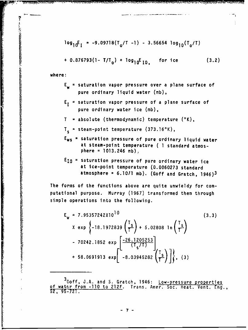
log 1 E = -9.09718(T /T -1) - 3.56654 loglO(To/T)
+ 0.876793(1- T/T0 ) + log 0E1io, for ice (3.2)
where:
Ew = saturation vapor pressure over a plane surface of
pure ordinary liquid water (mb),
EI = saturation vapor pressure of a plane surface of
pure ordinary water ice (mb),
T = absolute (thermodynamic) temperature (OK),
Ts = steam-point temperature (373.16 0K),
Ews = saturation pressure of pure ordinary liquid waterat steam-point temperature ( 1 standard atmos-phere = 1013.246 mb),
EJo= saturation pressure of pure ordinary water ice
at ice-point temperature (0.0060273 standardatmosphere = 6.1011 mb). (Goff and Gratch, 1946)3
The forms of the functions above are quite unwieldy for com-
putational purpose. Murray (1967) transformed them through
simple operations into the following.
Ew = 7.95357242X0 1 TO (3.3)
X exp 1-8.1972839 (is 5.02808 lnT
- 70242.1852 exp "(6T s/T ]
+ 58.0691913 exp [ 8.03945282 (T-)Js (3)
3Goff, J.A. and S. Gratch, 1946: Low-pressure propertiesof wate.r from -110 to 212F. Trans. Amer. Soc. Heat. Vent. Eng.,52,' 95'-721.
-7-
and
Ei 5.75185606X10 1 0 exp -20.947031 (0~-(5_o) 2.01889049 (4)
3.56654 in- (T0/T) 2
Goff and Gratch (1946) claimed a 2XO " percent
uncertainty for the water reference formulation, Eq. (3.1),
(above 0 0C) and 3Xl0 "2 percent for the ice reference formula-
tion, Eq. (3.2). The uncertainty value for water reference
does not apply to values below OOC where no experimental data
were available. Values in the range of 0 to -500C were
derived by direct extrapolation.
Murray's reformulations, Eqs. (3.3) and (3.4), of the
Goff-Gratch formulas differed from the original Goff-Gratch
Eqs. (3.1) and (3.2) by a maximum of 6X10 5 percent (at -250C)
and 3X10 5 percent (at -200C) for water and ice references
respectively.
4. TETENS' FORMULAS
Murray's transformations of the original Goff-Gratch
equations are still rather unwieldy from the standpoint of ease
of computation. In this respect, the transforms, Eqs. (3.3)
and (3.4), gain little over the original. A simpler formulation
for determining these values is highly desirable. The formula-
tion most used in the field of meteorology has been and is that
of Magnus. Tet~ns (1930) 4 gave this as
logoE5 tu + w (4.1)l~glo~s t+v
4Tetdns, 0., 1930: Uber einige meteorologische Begriffe.Z. Geophys., 6, 297-309.
-8-
where t is the temperature (0C), w = 0.7858 for vapor pressurein mb, and
u = 9.5 for ice; and u =7.5 over water.
v = 265.5 v = 237.3
A later statement of this formula can be fodnd in Haurwitz
(1945) 5 and is given as
(ut)E = 6.1078 X 10 ( +- (4.2)
where u, v and t have the values and meanings given above.
Murray (1967), for the purpose of achieving greater ease
and speed of computation, reformulated Eq. (4.2) to
Es = 6.1078 exp (4.3)" (T-bi
where T is temperature (OK), and
a = 21.8745584 a = 17.2693882for ice; for water.
b = 7.66 b = 35.86
Murray (1967) showed that the maximum difference between the
Goff-Gratch and Tet~ns formulation, for both ice and water,was well within the degree of uncertainty demonstrated by
Goff and Gratch (1946). The amount of error (or difference)
arisi:ig from the use of Tetgns formulation, Eq. (4.3), can beseen in Table 1 for water and Table 2 for ice. The maximum
er-or (difference) for water is 4.4 percent at -500C, and,
for ice is 3.0 percent at -50C.
6Haurwitz, B., 1945, Dynamic Meteorology, New York, N. Y.,McGraw-Hill, pp.
5. TABLE LOOK-UP PROCEDURE
In addition to the procedures discussed in the preceding
sections, there is another method for computing saturation
vapor pressure which is quite popular. This is the method of
"table look-up." It is particularly attractive when consider-
able computer memory is ave 4lable to a programmer. The "table
look-up" procedure requires the storage of tabular values of
saturation vapor pressure over a desired range of temperature.
This stored table becomes a permanent and integral part of the
program.
For a given temperature, limits of saturation vapor
pressure are chosen from the table. This is accomplished by
determining the algebraically largest tabular value of tempera-
ture less than the temperature in question. The saturation
vapor pressures for this and the next higher tabular entries
are chosen for limits (e.g., in a table of vapor pressure
values for each whole degree temperature, for a temperature of
6.55°C, the limits will be the vapor pressure values f: 60C
and 7C). The required value of vapor pressure is thei deter-
mined by linear (or higher order) interpolation within these
limits. Linear interpolation is normally sufficient because
values of vapor pressure between those for integer values of
temperature are closely approximated by a straight line.
The accuracy attained by this procedure is very acceptable
(see Table 1) with the largest error occurring at the middle
of a tabular interval (i.e., at (T + 0.5)°C for a table of
values at 10C tabular intervals). The "table look-up" method
is more accurate than the Tet6ns' formulations for temperatures
less than -5°C and usually less accurate for those above -51C
(using Goff-Gratch as the standard). It is slightly more
accurate than the polynomial procedures (see section 6) from
-50 to -25°C but less accurate above -250C.
-10-
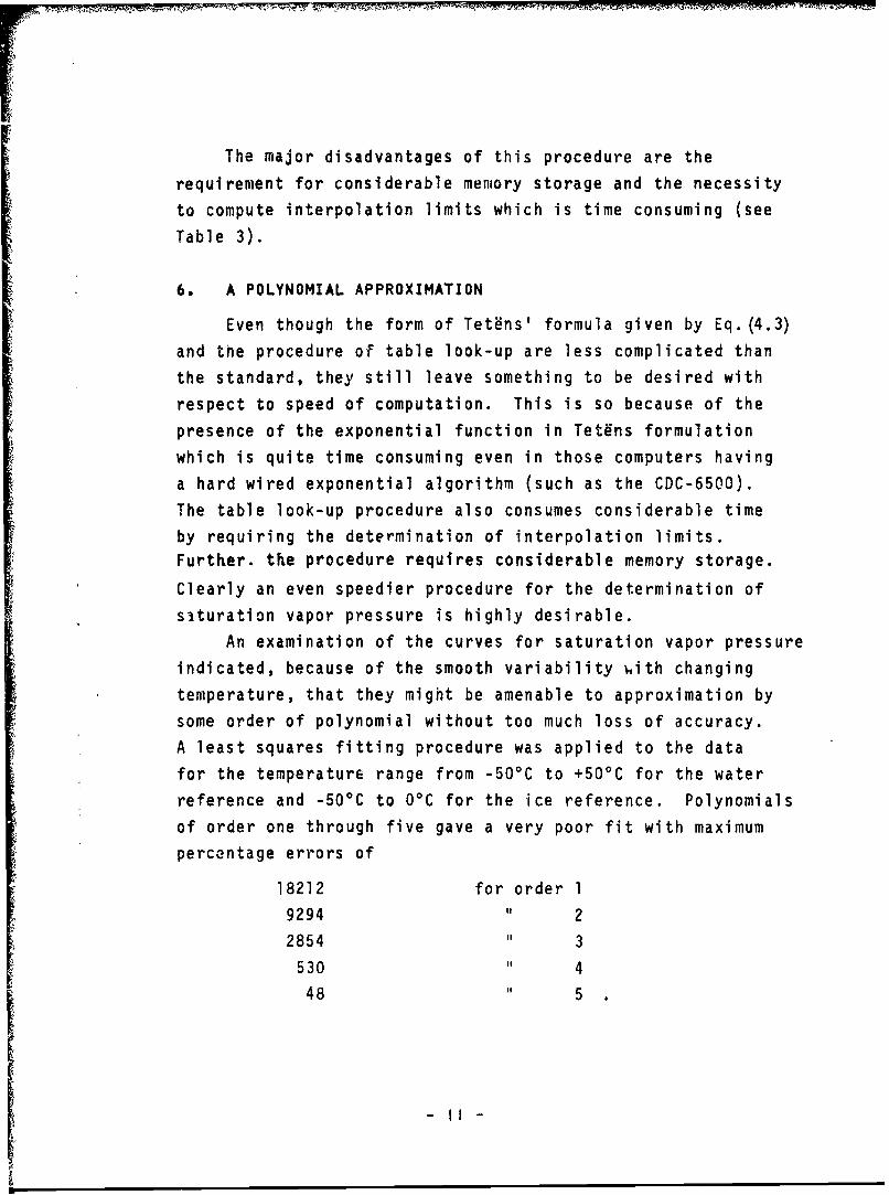
The major disadvantages of this procedure are the
requirement for considerable memory storage and the necessityto compute interpolation limits which is time consuming (see
Table 3).
6. A POLYNOMIAL APPROXIMATION
Even though the form of Tetdns' formula given by Eq.(4.3)
and the procedure of table look-up are less complicated than
the standard, they still leave something to be desired with
respect to speed of computation. This is so because of the
presence of the exponential function in Tetgns formulation
which is quite time consuming even in those computers having
a hard wired exponential algorithm (such as the CDC-6500).The table look-up procedure also consumes considerable time
by requiring the determination of interpolation limits.
Further. the procedure requires considerable memory storage.
Clearly an even speedier procedure for the determination of
situration vapor pressure is highly desirable.
An examination of the curves for saturation vapor pressure
indicated, because of the smooth variability ith changing
temperature, that they might be amenable to approximation by
some order of polynomial without too much loss of accuracy.
A least squares fitting procedure was applied to the data
for the temperature range from -500C to +50°C for the water
reference and -500C to O°C for the ice reference. Polynomials
of order one through five gave a very poor fit with maximum
percentage errors of
18212 for order 19294 2
2854 3
530 i" 4
48 5
- I I -
All of these percentage errors occurred at -500C (for the
water reference). The maximum percentage errors for the icereference for polynomials of order one through five are
1540 for order 1
601 2149 326 42.6 5
The sixth order polynomials for both the ice dnd liquid
water reference gave errors of less than one percent forthe entire meteorological range of Interest. The polynomialformulation for saturation vapor pressure is
Es = ao + t (a1+t(a2+t(a3+t(a4+t(a5+a6t))))), (6.1)
where t is temperature in degrees centigrade* and the constantshave the following values
for water for ice
ao = 6.107799961 ao = 6.109177956
a1 = 4.436518521X10 a, = 5.034698970X10"2- .294851 2 -2
a2 1.428945805X10 a2 = 1.886013408X10"
a3 2 2.650648471X10 - 4 a3 = 4.176223716X10 4
a4 = 3.031240396X10 6 a = 5.824720280X10 6
a5 = 2.034080948X10 8 a4 4.838803174X10 8
a6 = 6.136820929X101 a 5 1.838826904X0 10
66 = l88294l 1
(Range of validity: -500C to +500 C for water, -5CC + O°Cfor ice)
The coefficients can be readily re-evaluated for usewith temperatures in degrees Kelvin.
-12 -
7. ACCURACY RELATIVE TO THE ACCEPTED STANDARD
Table 1 gives valiues of saturation vapor pressure (over
water) as calculated by the Goff-Gratch formulation (EG),
Eq. (3.1); by Tetgns' formula (ET), Eq. (4.3); by table look-up
(ETL); and by the polynomial (EL) , Eq. (6.1). Also shown in
Table 1 are values of percentage departure (error) of the
Tetgns formula and polynomial results from the Goff-Gratch
standard. These percentages are indicated by the values in
parentheses. Table 2 gives analogous information for satura-
tion vapor pressure with respect to a plane ice surface. A
quick examination of these tables indicates that, with only
one exception (OWC, for ice, Table 2), the percentage departure
due to the polynomial procedure is everywhere many times less
than that due to the Tet~ns formulation. Therefore, as Murray
(1967) has shown, saturation vapor pressure values determined
by Tetgns formula, Eq. (4.3), depart from the standard by amounts
less than the degree of uncertainty embodied in the standard.
The polynomial values which have smaller departures must be
even further within the zone of uncertainty.
Having shown that the polynomial yields values of satura-
tion vapor pressure which are at least as accurate as the
Tetgns formulations, it is next necessary to inquire into the
relative speeds of computation of the methods discussed above.
Each of the procedures was used to compute a set of 10,000
saturation vapor pressures. Evaluations were made on two
computer systems -- the CDC 3100 and the CDC 7600. The results
of these evaluations are shown in Table 3.
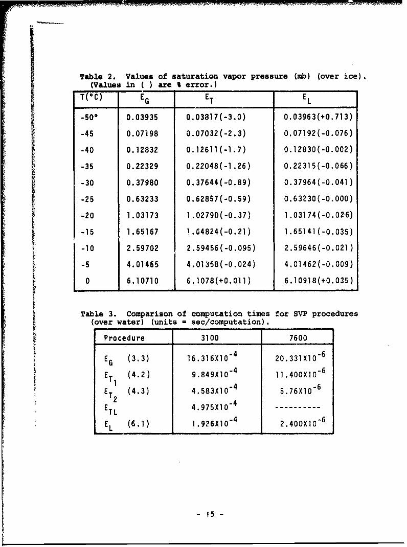
From Table 3, it can be seen that the polynomial formula-
tion is approximately 2.5 times faster than the best Tetgns
formulation. It would seem, then, that the demonstrated
accuracy and speed would justify the use of the polynomial for
the determination of saturation vapor pressure in numerical
models.
- 13 -
ITable 1. Values of saturation vapor pressure (in ub) (overwater). (values in 0) are 4 error.)
*Temperature for this column are offset upwards by 1/2 degree, i.e., the 03Centry is really the value for +0.50C.
-14 -
Table 2. Values of saturation vapor pressure (mb) (over ice).(Values in ( ) are % error.)
T(C) EG ET EL
-50@ 0.03935 0.03817(-3.0) 0.03963(+0.713)
-45 0.07198 0.07032(-2.3) 0,07192(-0.076)
-40 0.12832 0.12611(-1.7) 0.12830(-0.002)
-35 0.22329 0.22048(-1.26) 0.22315(-0.066)
-30 0.37980 0.37644(-0.89) 0.37964(-0.041)
-25 0.63233 0.62857(-0.59) 0.63230(-0.000)
-20 1.03173 1.02790(-0.37) 1.03174(-0.026)
-15 1.65167 1A.4824(-0.21 ) 1.65141 (-0.035)
-10 2.59702 2.59456(-0.095) 2.59646(-0.021)
-5 4.01465 4.01358(-0.024) 4.01462(-0.009)
0 6.10710 6.1078(+0.011) 6.10918(+0.035)
Table 3. Comparison of computation times for SVP procedures(over water) (units = sec/computation).
Procedure 3100 7600
EG (3.3) 16.316X10 4 20.331X10 6
ET (4.2) 9.849X10 4 11.400X10 6
1ET (4.3) 4.583X10 5.76X10 6
~2
E TL 4.975X10 "4
EL (6.1) 1.926X10 4 2.400XI0 6
-15-
8. COMPUTATION OF THE DERIVATIVE WITH RESPECT TO TEMPERATURE
Many thermodynamic computations necessary for atmospheric
simulation require determination of values of the derivative
of saturation vapor pressure with respect to temperature.
Differentiation of the Goff-Gratch equations as reformulated
by Murray (see Eqs. 3.3 and 3.4) yields
[E = 5.02808 18.1973 + 446.844 exp 8.039 (8.1)
Ts T 1834762 26.1205 ] Ew
(Tr)) (T_) 1834762 exp (/
for liquid
dE r T 2.01891] E,r 20.947(T-) + 3.56654 - (T/T) JT- for ice (8.2)
(Murray & Hollinden, 1966)6
It can be seen that these expressions are much more complicated
than even the original Goff-Gratch equations. Besides the
complication of form, it is also required to calculate the
saturation vapor pressure itself, if it is not already known --
which is not likely.
Logarithmic differentiation of Tetgns' formula, Eq. (4.3),
gives
dES A'E5 (8.3)
T- 2 where A' = 5807.71 over ice and 4098.03
over water
B = 35.86 over water and 7.66 over
ice.
6Murray, F.W. and A.B. Hollinden, 1966: The evaluation
of cumulus clouds: A numerical simulation and its comearison
against observations. Douglas Aircraft Co. Rep. #SM-49372.
-16-
This expression would lead to a very rapid calculation of the
derivative if Es is known. If it is not, then the calculation
will be s1ihtly more lengthy, than Tetfns' calculation for
saturation vapor pressure,An attempt was made to fit a polynomial to values of the
Iderivative over the range of temperatures of meteorologicalinterest. The data used was obtained by evaluations of Eqs.(8.1) and (&2). Polynomials of order 5, 6 and 7 all showed
acceptable error patterns (i.e., errors less than those arising
I from the Tet~ns formulation, Eq. (8.3))for water. For iceI reference, orders 5 and 6 were acceptable, but strangely enoughhigher orders were not. An evaluation of mean, maximum androot-mean-square errors indicated that the sixth order polyno-
Imial was again the optimum choice. The polynomials take thesame form as Eq. (6.1) but with coefficients as shown below:
for water for ice (8.4)
ao a 4.438099984XlO " ao = 5.030306237XI0 "
aI a 2.857002636X10² a1 - 3.773255020X10 2
a2 n 7.938054040Xi0-4 a2 = 1.267995369X10 3
a 3 - 1.215215065XI0 "5 a 3 = 2.477563108X10"5
a4 = 1.036561403X10 7 a4 = 3.005693132X10 7
a5 = 3.532421810X10 10 a, = 2.158542548X10 9
a6 --7.090244804X10 13 a6 = 7.131097725X10 12
(range of validity: -500C to +500C for water;
-50'C toO°IC for ice)
-'7-
dEs
Table 4 shows the values of a as computed using the Goff-
Gratch (DG) derivatives, Tetgns' derivative (DT), and those
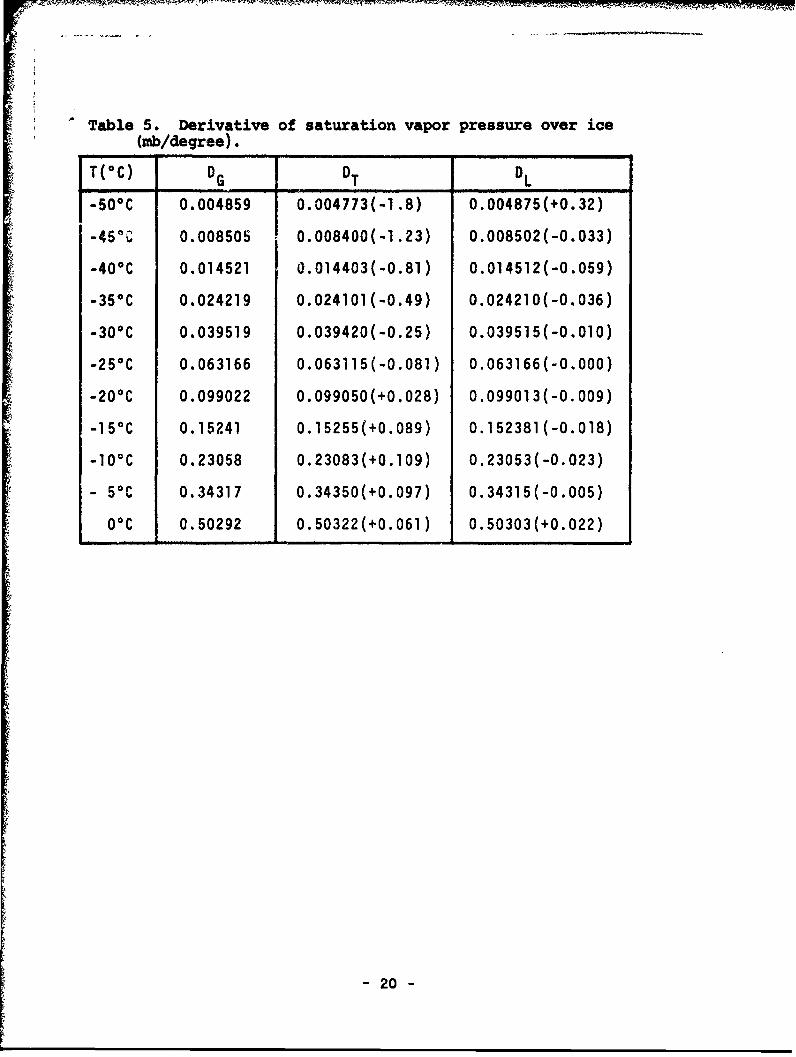
determined from the polynomial (D1) just discussed. Table 5
shows similar information for dEs/dT for the ice reference
case. As with the primary functions, the polynomial expres-
sions, coefficient set (8.4), for the derivatives (with
reference to both ice and water) show departures (errors)
from the Goff-Gratch standard which are considerably less than
those determined by the use of Tetgns' formulation, Eq. (8.3).
Derivative computation times are comparable (as would be
expected) to those for the primary expressions for saturation
vapor pressure (see Table 3).
9. SUMMARY
It has been shown that it is possible to formulate a
polynomial approximation for both saturation vapor pressure
and its derivative with respect to temperature that is at
least and 's generally much more accurate than currently used
procedures (Tetgns' formula). Accuracy was measured in terms
of departure from values derived from the Goff-Gratch formulas
which are the internationally accepted standards. The poly-
nomial errors are well within the degree of uncertainty
connected with the Goff-Gratch procedures. The polynomial
procedures have been demcnstrated to consume significantly
less computer time that methods currently in use. The employ-
ment of this procedure will result In significant savings in
the consumption of computer resources and money. These same
polynomials may be used to evaluate actual vapor pressure by
using the dew point temperature in lieu of air temperature.
- 18 -
Table 4. Derivative of saturation vapor pressure over water(mb/degree).
T(0C) D G D T D L
-500C 0.007286 0.007100(-2.6) 0.007188(-1.35)
-450C 0.012113 0.011897(-1.8) 0.012234(+1 .001)
-400C 0.019624 0.019394(-1.17) 0.019644(+0.099)
-350C 0.031042 0.030824(-0.70) 0.030940(-0.329)
-300C 0.048021 0.047849(-0.36) 0.047887(-0.279)
-250C 0.072756 0.072673(-0.11) 0.072678(-0.107)
-200C 0.10811 0.10816(+0.045) 0.10812(+0.013)
-15 0C 0.15773 0.15795(+0.136) 0.15782(+0.059)
-100C 0.22622 0.22662(+0.176) 0.22634(+.052)
-5oC 0.31927 0.31983(+0.1 79) 0.31935(+.025)
00C 0.44381 0.44449(+.154) 0.44381(0.00)
50C 0.60817 0.60886(0.114) 0.60809(-0.013)
100C 0.82225 0.82279(0.065) 0.82211(-0.016)
150C 1.0976 1.0978(0.016) 1.0975(-0.010)
200C 1.4477 1.4473(-0.028) 1.4476(-0.005)
240C 1.8878 1 .8867(-0.063) 1 .8878(+0.002)
300C 2.4354 2.4334(-0.083) 2.4355(+0.003)
350C 3.1100 3. 1072(-0.087) 3. 1100(-0.0002)
400C 3.9331 3.9303(-0.072) 3.9331(-.0009)
45%C 4.9287 4.92691-0.036) 4.9286(-0.001)
500C 6.1228 6.1241(+.022) 6.1230(+.003)
-19-
Table 5. Derivative of saturation vapor pressure over ice(mb/degree).
T(OC) j D T D L-500C 0.004859 0.004773(-1.8) 0.004875(+0.32)-450C 0.008505 0.008400(-1.23) 0.008502(-0.033)