DISTRIBUTED BY: National Technical Information … · TOTAL NO OF P.GEv Tb NO 1)F pEPr$ ... or...

AD-A007 269

MONOPOLE ANTENNA WITH A FINITE GROUNDPLANE IN THE PRESENCE OF AN INFINITEGROUND

Sang-Bin Rhee

Michigan University

Prepared for:

Army Electronics Command

November 1967

DISTRIBUTED BY:

National Technical Information ServiceU. S. DEPARTMENT OF COMMERCE

NOTICES

Disclaimers

The findings in this report are not to be construed as anofficial Department of the Army position, unless so desig-nated by other authorized documents.

The citation of trade names and names of manufacturers inthis report is not to be construed as offic. al Governmentindorsement or approval of commertial products or servicesreferenced herein.

Disposition

Destroy this report when it is no longer needed. Do notreturn it;to the originator.

--- --- --

, 2;e ..

lto1I t * €

LIIa

Security Classification 19 ~2DOCUMENT CONTROL DATA- R&D '

(Security clteifltcti-v, of title. body of abstract end indes annofalton mut be entered wAen he overall #.;Pot Jsl leashed)

I ORIGINATING ACTIVIvY (Conporate author) 24 REPORT SECURlTY C LAMII^CA TIONCooley Electronics Laboratory UnclassifiedThe University of Michigan Zb GROUPAnn Arbor, MichiganI

I REPORT TITLEMonopole Antenna With a Finite Ground Plane in the Presence of An InfiniteGround

4 DESCRIPTIVE NOTES (Type of report end inclusive date*)Supplemental Technical Report May 1966 to July 1967

S AUTHOR(S) (Last nSeM. first nm, Initill)

Rhee, Sang-Bin

6 REPOPY DATE 7. TOTAL NO OF P.GEv Tb NO 1)F pEPr$

November 1967 - /, 18$a CONTRACT OR0 GRANT NO 90 ORIGINATOWS REPORT NUMBER(S)

DA 28-043-AMC-02246(E)b PROJECT NO 8107-5-T

5A6-79191-D902-02-24c S b O~ ~ ~~ ~~th Ei Iq P O A T N O (S) (A ty o th o r m u a :e $ thlny b e l ~ l e

ECOM-02246-5 j

10 AVAILADUTY /L miTON NOTICES copies ol ths repor may e ine m eto , N * na d riL ncj0 . pa 207 e n: Ec

I I SUPPL"EETARY NoTEs AMSEL-WL-S ':2 SPONSORING .,airARY ACTIVITYU. S. Army Electronics Command

Fort Mc;amouth, N. J. 07703Attn: AMSEL-WL-S

13 ABSTRACT An experimental and theoretical study was made of a monopole antennamounted on a finite ground plane located above an infinite ground. Circular flatdiscs and hemispheres were used for the finite ground planes. Experiments wereconducted over a 6 to 1 frequency range, with the length of monopoie antennafixed at a quartei wavelength at the upper end of the frequency band. The radiiof finite ground planes used for experiments were generally le:ss than a quarterwavelength.

Input i pedances were measured as a function of frequency at the baseof the antenna, using as variables the radius and the locations of the ground planewith respect to an infinite ground below

A theoretical analysis is also made of a monopole with a hemisphericalground plane on an in, ite ground. Far zone electromagnetic fields were calcu-lated as a function of both the ground plane radius and the frequency. Radiationresistances were also calculated.

The results of the study indicate that the radiation resistance of anelectrically short antenna may be increased significantly by locating it on aground. This conclusion opens the way for a more efficient utilization of receiv..ing and transmiting antennas on ground-based vehicles. The impedance charac-teristics of the antenna system are such as to facilitate its operation over a broadfrequency range.

FOIDD , ANR1,1473 R-,dcdb

NATIONAL TECHNICAL Security ClassificatonINFORMATION Qyljwl:

Security Classification _______

114 KYWRSLINK A LINK B IN

______________________________ ROLE W___ j fOLC wr ROLE WFinite Ground Plane imHemispherical GroundBroad BandingRadiation ResistanceCurrent DistributionInput ImpedanceVehicular Mounted AnteponaEquivalent CircuitElectrically Short Antenna

INSTRUCTIONS

1. ORIGINATING ACTI'VITY: Enter the name and address Imposed by security classification, using standard statement;Iof the contractor, subcontractor, grantee, Department of De- such as-

tense activity or other organization (corporate author) issuingt (1 "Qa fe requesters may obtain copies of thisthe rport.report from DDC "

2a. REPORT SECUITY CLASSIFICATION: Enter the over- (2) " Foreign announcement and disseminat:.,.i of thisall security classification of the report. Indicate whetherreotb Disntahrzd."Restricted Date" is included. Marking is to be in accord-rpotbDD isntahrid"

itance with appropriate security regulations. (3) "U. S. Government agencies m.y obtain copies ofthis report directly from DDC. Other qualified DDC2b. GROUP: Automatic downgrading is specified in DoD Di. users shall request through

rective 5200. 10 and Armed Forces Industrial Manual. Enterthe group numbe - Also, when applicable, show that ptional _______________________

markings have oeen used for Group 3 and Group 1 as author- 4) "U. S. mi irary agencies nay obtain copies of thisized report directly from DDC Other qualified users

3. REPORT TITLE: Enter ine complete report title in all %hall request throughcapital letters. Titles in all case-s should be unclassified.IU a meaningful title cannot be selected without cl&isifice-tion, show title classification in all LapitaliS in par -nthesis (5), "All distribution of this report is controlled. Qual-immediately following the title. ited A.iDC users shall requ~est through4. DESCRIPTIVE NOTES: If approp'.a'e. v .,er the type of ~_________report, e.g., interim, progress. summary., aiinuail, or f, -al. If the -eporz'n os Leer furrusho'd to the Office of TechnicalGive t1'e inclusive dates when a specific reporting period is Services. Departmrent of Conimerce, for sale to the public, indi-covered. c-ate this fact and entuer the price, if known.5. AUTHOR(S). Enter the nne~s) of alithor(s) as shown on 11. SUPPLF.MLNTAiRY NOTES Use for additional explana-or in the report. Enici last name, first name, middle initial, 'o:y notes.If -rilitary, show rank and branch of service. The -,ame ofthe principal . 'thor ih an absolute minimuim reqwrement. 12. SPONSORING MILITARY ACTIVITY: Enter the name of

6. RPOR DAE. nte th dae o th reortas ay, the departmental project office or saboratory sponsoring (put,-mnonlh, year, or month, year. If more than one dute appeara b ~ fr h eerhaddvlpet nld ir-son the report, use date of publication, 13 ABSTRACT Enter an abstract &lyingt a brief and fat tual

7.. OTA NUBEROF ACESThetotl pge oun summary of the docurnt indicative of the report, even though7e. OTA NUBER F PCESThetota pae cunt it may also appear elsev-..-e in the body of the technica! -

shauld follow normal pagination procedures, i.e., enter the port If additional sp~eis reqnird, a continuation sheet shallnumber of pages containing information. be attacheO76. NU'MBER OF REFERENCES. Unter the total number of It is highly desirable that the abstract of classified reportsreferences cited in the report. be unclassified Each paragraph of the abstract shall end with8a CONTRACT OR GRANT NUMBER. If appropriate, enter an indication of the mialitury tocurity classification of the inthe applicable number of the contract or grant under which formation in the paragrap'i represented as (rS,1 (S) (C) IU

tereport was writter. There is no li'niiatmorn on the length of the abstract Ho%%8b, 8c, & 8d. PROJECT NUMBER. Enter the appropriate ever, the suggested length Lf; irom ISO to 225 wordsmilitary department identification, such as project number,subproject number, system numbeis, task number, etc. 14s KE) WORDS. Key words are technit-ally rmeuninqfu terws

or stgr ph ro:.eii that hero( tenire a report and muN be usePd as9a. ORIGINATOR'S REPOR * NUM8BER(S. Enter the offi- index entries~ fu .ataloging the report Key worcis must becial report number by which the docimevnt will he identified sele( ted so that no sec-urity lsis;nihbo.i is required Identiand controlled by the originatin;, aivity. Thin t-umber mrust fiers, suc-h an equipmeni model ilcsignatiun trade name rithtar-,

1be unique to this report. projec f r de nanie yeog aphi( ccaimon nvs be used a% ke19b. OTHER REPORT NUM2I1-R( ), If the report has been word%, hut w-11 hi- follow2-d by 6-, in-to ,iiicn of i'r-b'ca! Lon

assigned any other repcrt nunber', (either bj, the originator tetT- sirnir olri re ndwitsi14i.IRor by, the &ponsor). also enter this number(s).

10. AVAILAEILITY/I.IMITATION NOTICES- Enter any hinT-

tations on further disseninaion of the report, other than those(

Reports Control SymbolOSD 1366

V

Technica! Report ECOM-02246-5 November 1967

MONOPOLE ANTENNA WITH A FINITE GROUND PLANE IN THEPRESENCE OF AN INFINITE GROUND

Report No. I

Supplemental Tecnnical Report

Contract No. DA 28-043 AMC-02246(E)

DA Project No. 5A6-79191-D902-02-24

Prepared by

Sang- Bin Rhee

COOLEY ELECTRONICS LABORATORYDepartment of Electrical Engineering

The University of MichiganAnn Arbor, Michigan

for

U.S. Army Electronics Command, Fort Monmouth, N.J.

DISTRIBUTION STATEMENT

h " do

0"I utli Je~r

ABSTRACT

An experimental and theoretical study was made of a mono-

pole antenna mounted on a finite ground plane located above an infinite

ground. Circular flat discs and hemispheres were used for the finite

ground planes. Experiments were conducted over a 6 to 1 frequency

range, with the length of monopole antenna fixed at a quarter wave-

length at the upper end of the frequency band. The radii of finite

ground planes used for experiments were generally less than a quarter

wavelength.

Input impedances were measured as a function of frequency

at the base of the antenna, using as variables the radius and the locations

of the ground plane with respect to an infinite ground below. Scale

models were used to obtain measurements of radiation patterns and

antenna current distributions. Results of these measurements are

presented graphically.

A theoretical analysis was also made of a monopole with a

hemispherical ground plane on an infinite giound. Far-zone electro-

magnetic fields were calculated as a function of both the ground plane

radius and the frequency. Radiation resistances were also calculated.

The results of the study indicate that the radiation resistance

of an electrically short antenna may be increased significantly by

locating it on a small ground plane above the infinite ground, rather

than directly on the infinite ground. This conclusion opens the way for

iii

a more efficient utilization of receiving and transmitting antennas on

ground- hbsed vehicles. The impedance characteristics of the antenna

system art: such as to facilitate its operation over a broad frequency

range.

iv

FOREWORD

This report was prepared by the Cooley Electronics Labora-

tory of The University of Michigan under United States Army Electronics

Command Contract No. DA 28-043-AMC-02246(E), Project No. 5A6-79191-

D902-02-24, "Improved Antenna Techniques Study."

The research under this contract consists in part of an

investigation to develop highly efficient remotely tuned impedance match-

ing coupling networks for electrically short monopoles.

The material reported herein represents a summary of a

theoretical and e4'-perimental study which was made to determine the input

impedance and radiation characteristics of an electrically short monopole

over a small ground plane located at various distances above natural

ground.

m

TABLE OF CONTENTS

Page

ABSTRACT iii

FOREWORD v

LIST OF TABLES viii

LIST OF SYMBOLS ix

LIST OF ILLUSTRATIONS xv

LIST OF APPENDICES XX

I. INTRODUCTION 1

1. 1 Statement of the Problem I1. 2 Topics of Investigation 21.3 ileview of the Literature 41. 4 1 hesis Organk-ation 5

II. INPUT IMPEDANCE MEASUREMENT 82.1 Introduction 82.2 Experimental Measurement Procedure 82.3 Scale Model Impedance Measurements 202.4 Results of Mea-urement 262. 5 Copper Losses Ptue to the Antenna and 39

the Ground Plane2. 5. 1 The Interna, Impedance of the Plane 41

inductor2. 5. 2 Internal Impedaince of a Conductor with 45

a Circular Crosz Section2. 5. 2. 1 Currel't Ln a Wire of a Circular 45

Cross Section2. 5. 2. 2 The Internal Impedance of a 49

Round Wire

III. CURRENT MEASURFMENTS 543. 1 Introduction 543.2 Theory of Current Probe 543.3 Experimental Procedures 613. 4 Measurement Results 68

vi

TABLE OF CONTENTS (Cont.)

Page

IV. RADIATION PATTERN MEASUREMENTS 864.1 Intrnduction 864.2 Measurement Problems 864. 3 Experimental Technique 884.4 Measurement Results 93

V. THEORETICAL ANALYSIS 1065. 1 Introduction 1065. 2 General Far-Zone Field Expressions 107

5. 2. 1 Classical Formulation 1075. 2. 2 Stratton-Chu Integral Formulation 117

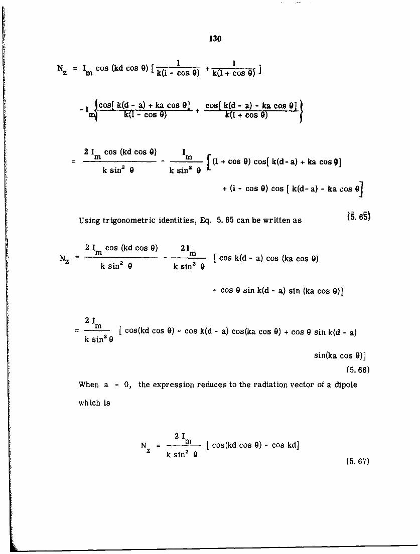
5.3 Far-Zone Field Expressions for Two Linear 1 26Antennas

5.4 Induced Current on a Spherical Surface 1325. 4. 1 Induced Current on a Conducting Sphere 132

Excited by a Monopole5. 4. 2 Induced Current Due to the Image Antenna 141

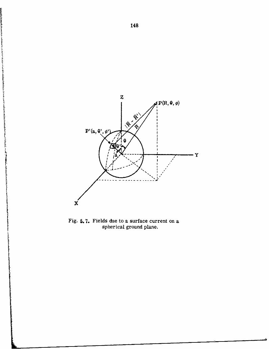
5.5 Far-Field Expressions Due to a Spherical Surface 147Current Distribution5. 5. 1 Evaluation of l 1575. 5. 2 Numer:cal Evaluation of a Radiation Pattern 162

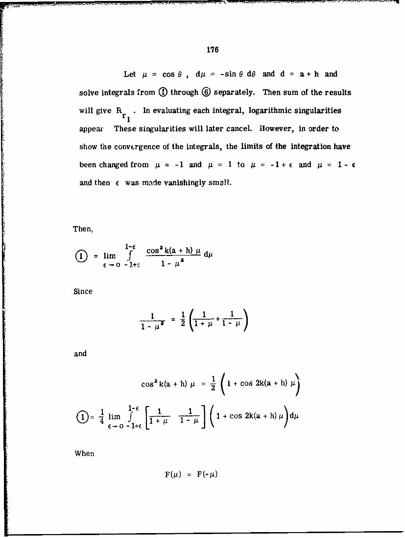
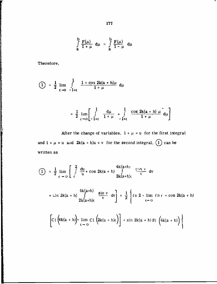
5.6 Ra' ,iti-,,n Resistance 1715. 6. 1 r,' , w.aion of R 174

5. 6. 2 Eva uation of P 183

5.6.3 Evaluation of R 184r3

VI. CONCLUSIONS AND RECOMMENDATIONS 1956. 1 Conclusions 1956.2 Recommendation for Future Work 198

REFERENCES 216

DISrRIBUTION LIST 218

vii

LIST OF TABLES

Table Page

2. 1 Scale factors 21

5. 1 Ratios of in(W)164

5.2 Coefficients B" 165n

viii

LIST OF SYMBOLS

FirstSymboi Meaning_ Appeared

5 electromagnetic waves depth of

penetration 10

Z characteristic impedance of ai: 0

transmission line 14

ZL load impedance 14

Zd impedance at a distance d from a

load 14

free space wavelength 14

d distance measured from load 14

a electric conductivity 21

a i) distance between ar, jifinite ground

plane and a finite ground plane 25

ii) radius of a semisphere

P radiation resistance 39r

I input current 39

E electric field intensity vector 39

H magnetic field intensity vector 39

H4* complex conjugate of H 39

Re Real part of .... 39

R ground terminal resistance 40

ix

LIST OF SYMBOLS (Cont.)

First

Symbol Meaning Appeared

Rt resistance cf tuning units 40

R resistance of equivalent insulation loss 40

Rw resistance of equivalent conductor loss 40

R transmission line losses 40

" surface current density 42

V gradient operator 41

partial differential opr':ator 41

t time 41

w radian frequency 41

V x curl operator 41

V divergence operator 41

p electric charge density 41

V2 Laplacian operator 41

E permittivity 41

p permeability 41

j 1-Y 41

iz component of surface current density i 48

Eo electric field intensity on the surface of a

conductor 41

x


FirstSymbol Meaning Appcared

T /jWIO" 42

f frequency 42

Jz current density per unit length 43

Z surface impedance 43s

Rs surface resistance 43

L. internal inductance of a plane conductor 43,

r radial distance in a cylindrical coordinate 45

x, y, z unit vectors 45

A constant, area of a loop 46

J Bessel function of order n 46nV

Ber(v) real part of J (--y- 47

closed line integral 48

i incident magnetic flux density vector 56

reradiated magnetic flux density vector 56

c speed of light 56

e induced voltage 57

k free space wave numbei, 57

hb effective height of a loop antenna 57

xi


FirstSymbol Meaning Appeared

Y admittance 570

d i incremental length 57

10 zero phase sequence current 57

I(1) first phase sequence current 58

he effective height of a dipole antenna 58

KE electric sensitivity 59

KB magnetic sensitivity 59

D diameter of a loop 59

cx proportional to ... 60

magnetic scalar potentials IIIm

R', 0', 0' spherical coordinates expressing

source points 113

electric radiation vector 115

magnetic radiation vector 115

spherical unit vectors 115

Nt transverse electric radiation vector 115

a scalar function 116

M t transverse magnetic radiation vector 117

vector functions of position 117

xii



S surface 1.7

fictitious magnetic current density 125m

a8 surface electric charge density 125

0 a sclar function 120

r i) distance between a source point and

an observation point 118

R, , ¢ spherical coordinates 118

J fictitious magnetic current density 118m

Pm fictitious magnet ; charge density 118

electric field intensity arising from the

actual current and charge 108

H' mag -ic field intensity arising from the

actual current and charge 108

electric field intensity arising from the

fictitious magnetic current and charge 108

H" magnetic field intensity arising from the

fictitious magnetic current and charge 108

electric vector potential 109

electric scalar potential 109

G free space Green's function 110

A magnetic vector potential 111

xiii



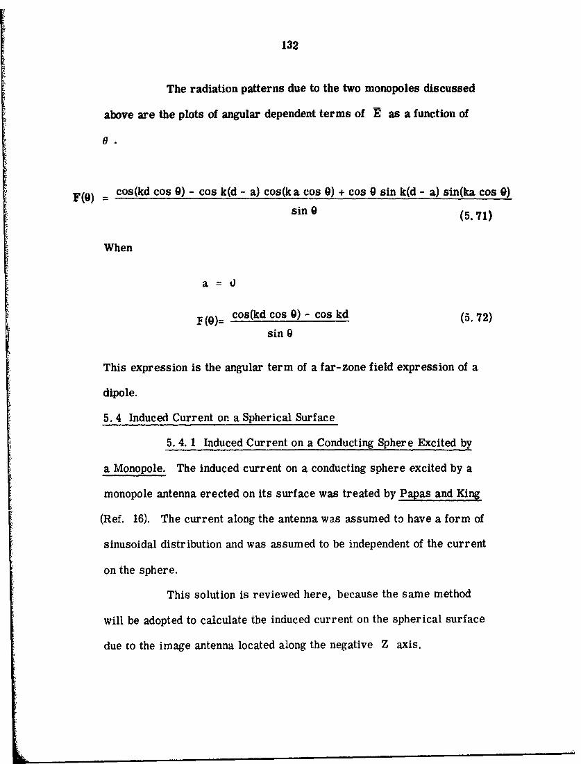
F(0) a scalar function 132

U a scalar f nction 138

Pn(COs 0) Legendre polynomials of order n 138

Pn (kR) weighted spherical Hankel function of

the second kind with order n 138

H (2)(kR) Hankel function of the second kind withnorder n 139

h(2)(kR) spherical Hankel function of the secondn

kind with order n 139

n (kR) spherical Bessel function with order n 151nn

Y n(0), 0) spherical surface harmonics of degree

n 151

factorial 151

cm, dm constant coefficients of an infinite

series 152

temporary variable 154

m(cos 9) associated Legendre functions of thePn

first kind, order n , degree m 154

6 delta function 159n

1 .. ... ... ... ..... .... .... .. .... .

LIST OF ILLUSTRATIONS

Figure Title Page

1.1 Theoretical models 3

2. 1 Antenna on the variable height ground plane 9

2.2 Block diagram showing the impedance measure- 11ment setup

2.3 Antenna test site 12

2.4 A 2. 5 meter monopole antenna on a 2. 5 meterdiameter ground plane supported by a styrofoamsheet 13

2. 5 Test equipment arrangement for the impedancemeasurement 16

2.6 Location of the impedance measurement bridgerelative to the antenna base 17

2.7 Antenna located at 5 meters above the naturalground with 2. 5 meter diameter ground plane 19

2.8 Block diagram showing an impedance measurement

set-up for a scaled model antenna system 24

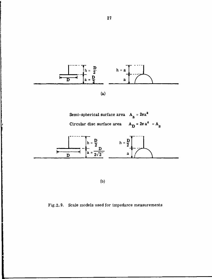
2.9 Scale models used for impedance measurements 27

2. 10(a) Input resistance as a function of frequency for aquarter wavelength monopole at 30 MHz on aninfinite ground plane 28

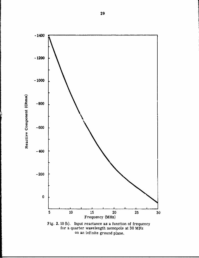
2. 10(b) Input reactance as a function of frequency for a quarterwavelength monopole at 30 MHz on an infinite groundplane 29

2.11 Input impedance versus frequency 30

2. 12 Input impedance versus frequency 31


xv

LIST OF ILLUSTRATIONS (Cont.)

Figure Title Page



2. 16 Input impedance versus frequency 35

2.17 An equivalent circuit of a monopole on a finitedisc ground plane above an infinite ground 38

3.1 Rectangular current loop 58

3.2 Circular loop probe 60

3.3 Current probe 63

3.4 Current measurement set-up 64

3. 5 Anechoic chamber 65

3.6 Block diagram for current measuremant set-up 66

3.7 Comparison of a sine curve with a current distri-bution of a monopole over a large ground plane 68

3.8 Theoretical current distribution of a monopoleon an infinite ground plane 69

3.9 Current distribution on a monopole antenna with afinite ground plane at various locations with respectto an infinite ground at 30 MHz 72

3. 10 Current distribiltion on a monopole antenna with afinite ground pktnt at various locations with respectto an infinite ground at 25 MHz 73



xv i


Figure Title Page

3.13 Current distribution on a monopole antenna witha finite ground plane at various locations withrespect to an infinite ground at 10 MHz 76

3.14 Current distribution on a monopole antenna witha finite ground plane at various locations withrespect to an infinite ground at 7.5 MHz 77

3.15 Current distribution on a monopole antenna witha ground plane of various diameters at a givenlocation with respect to an infinite ground at 30 MHz 78

3.16 Current distribution on a monopole antenna witha ground plane of various diameters at a givenlocation with respect to an infinite ground at 25 MHz 79

3.17 Current distribution on a monopole antenna witha ground plane of various diameters at a givenlocation with resuect to an infinite ground at 20 MHz 80

3.18 Current distribution on a monopole antenna witha ground plane of various diameters at a givenlocations with respect to an infinite ground at 15 MHz 81

. 19 Current distribution on a monopole antenna witha ground plane of various diameters at a givenlocation with respect to an infinite ground at 10 MHz 82

3.20 Current distribution on a monopole antenna witha ground plane of various diameters at a givenlocation with respect to an infinite ground at 7. 5 MHz 83

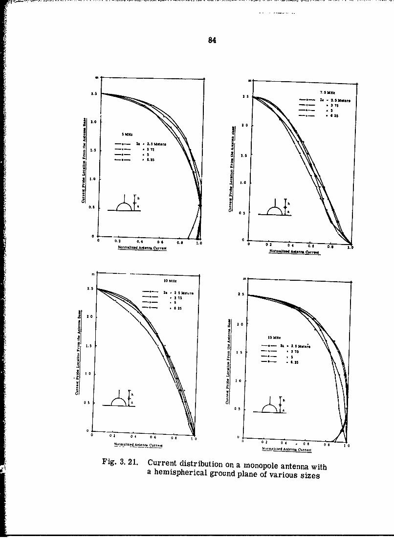
3.21 Current distribution on a monopole antenna witha hemispherical ground plane of various sizes 84

3.22 Current distribution on a monopole antenna with ahemispherical ground plane of various sizes 85

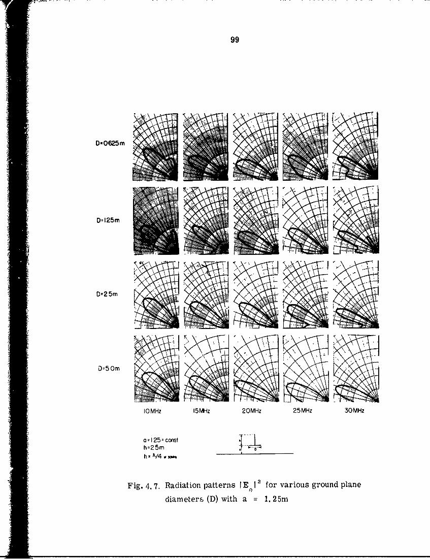
4. 1 Radiation patterns in the vertical plane 89

4. 2 Phase difference between center and edge of the 91test antenna

xvii


Figure Title

4.3 Radiation pattern measurement set-up,block diagram 96

4.4 Geometrical arrngement of an antennaand ground plane 94

4.5 Radiat gn patterns IE 0Z for a monopole with a

various 'iameters 97

4.6 Radiation patterns IE0 12 for various ground

plane diameters (D) with . = 0. 625m 98

4.7 Radiation patterns 1E 12 for various groundplane diameters (D) with a = 1. 25m 99

4.8 Radiation patterns ]E 0 12 for various ground

plane diameters (D) with a = 2. 5m 100

4.9 Radiation patterns IE0 12 for various ground

plane diameters (D) with a = 5. Om 101

4.10 Radiation patterns IE l for various ground

plane locations (a) with D = 0. 625m 102

4.11 Radiation patterns 1E 2 for various ground

plane locations (a) with D z 0. 25m 103

4.12 Radiation patterns I." 2 for various ground

plane locations (a) with D = 2. 50mn 104

4.13 Radiation patterns IE 0 1 for various ground

plane locations (2) with D = 5. Om 105

5. 1 Theoretical model of an antenna system 106

5, 2 Coordinate system used to derived far-zone 113electromagnetic fields

xviii


Figure Title Page

5. 3 Notations for Stok,'t's Lfeorem 11O

5. 4 Co-linear dipole 127

. 5 A monopole antenna above a spherical groundplane 133

5. 6 Image antenna with a cpherical ground plane 162

5.7 Fields due to a surface current on aspherical ground plane 148

5.8 Pn (cos ) versus 0 166

5.9 p (cos 0) versus 6 167n

5. 10 Theoretical radiation patterns IE 1 2 169

5. 11 Theoretical radiation resistances for variousvalues of ground plane size 188

5. 12 Theoretical radiation resistance and experimentalinput resistance for a monopole with a hemisphericalground plane 1.89

5. 13 Theoretical radiation resistance and experimentalinput resistance for a monopole with a hemisphericalground plane 190

xix

LIST OF APPENDICES

PageAPPENDIX A Reciprocity Theorem 201

APPENDIX B Proof and Derivation of Eq. 5. 56 203

APPENDIX C Proof of Eq. 5. 92 207

APPENDIX D Numerical Evaluation of B 212n

APPENDIX E Evaluation of R ir; Eq. 5. 168 214

xx

CHAPTER I

INTRODUCTION

Monopole and dipole antennas ovt:r an infinitely large con-

ducting ground plane are two of the oldest types of antennas being usea.

Their performance characteristics have been thoroughly studied in the

past. However, the exact behavior of the antenna over a conducting

ground plane of a finite size, and both antenna and finite ground plane

over infinite ground with finite r- nductivity has not been studied here-

tofore.

1. 1 Statement of the Problem

The purpose of this study is to investigate the properties

of a vertical monopole antenna and a finite ground plane locatd above

an infinite ground plane. Particular emphasis, in this investigation,

is placed upon the study of antenna systems having circular ground planes

ni which the dimensions of both the ground-plane diameters and the ground-

plan heights above infinite ground are smaller than the wavelengths

of intere.t.

The investigation of the prcpertic.s of this antenna system

provi6.'s a basis for a detailed comparison with the conventional antenna

systori of a monopole antenna over an infinite ground plane and for de-

termi',ation of the relative advantages and limitations of this system.

In o" ition, the re Its of this study will be applied to an investigation

of pos:sible performancp improvement for a monopole a~itenna mounted

2

on a ground-based vehicle, since there is reason to believe that the an-

tenna system proposed for study approximates the vehicular-mounted

antenna.

1. 2 Topics of Investigation

Since the purpose of this paper is to report a study of the

vertical monopole with a finite ground plane in the presence of an infi-

nite ground plane, the following topics are explored:

(1) The experimental measurement of the input impedance

of the antenna was carried out over the frequency range of 5 MHz to

30 MHz (a 6 to 1 band) and as a funct ion both of the ground-plane size

and of the ground-plane location, relative to an infinite ground.

(2) The experimental measurement of current distribution

on the antenna over the frequency range described above was carried

out with the ground plane size and its location as the variables.

(3) The radiation pattern was measured and its dependence

on the ground plane size and location was studied.

(4) A number of theoretical models was examined to deter-

mine a suitable approximation to the given system. Results oL.*ained from

the appropriate theoretical model was then c mpared with the experimen-

tal measurements.

One of the theoretical models which was studied is a mono-

pole placed on a semi-spherical conductor, as shovn in Fig. 1.

3

antenna

conduct'ngsemi- sphere

infinite ground

image

Fig. 1.1. Theoretical models

4

1. 3 Review of the Literature

Many studies of the properties of vertical monopole antennas

mounted both on infinite and on finite ground planes have previously been

reported in the literature.

Bardeen (Ref. 1), in 1930, studied the diffraction of a cir-

cularly symmetrical electromagnetic wave by a circular disc of infinite

conductivity. The result of his study has been usea in det ermmning the

power flow into the earth below a vertical antenna that is grounded by

a circular disc lying on the surface. In 1945, Brown and Woodward

(Ref. 2), in an experimental study, measured the resistance and reac-

tance of a cylindrical antenna operated against ground. The ground im-

mediately below the antenna had a buried metallic screen of a finite

size whose top surface was flush with the rest of the natural ground.

A particular emphasis was given to a study of impedance behavior as a

function of the antenna length to diameter ratio. Terminal conditions

such as capacitance of the base of the antenna to ground were considered.

Later, Meier and Summers (Ref. 2) (1949) performed an

experimental study of the impedance characteristics of vertical antennas

mounted on finite ground planes. Leitner and Spence (Ref. 3) (1951)

confirmed some of these experimental results through the theoretical

study of a quarter-wavelength monopole on a finite, circular-disc ground

plane. They assumed a sinusoidal current distribution to exist on the

antenna. The results of this study showed a marked dependence o the

antenna radiation resistance upon the diameter of the disc employed.

5

This dependence was particularly pronounced for small ground planes.

In 1951, Storer (Ref. 4) used a variational method to readily obtain the

expression for the dependence of the antenna impedance on the ground

plane diameter. Tang (Ref. 5), in 1962, further studied the radiation

pattern of this system by using the Babinet principle and the Wiener-Hopf

technique.

In each of the above papers, the monopole was considered to be

above a finite ground plane suspended in a free space with no direct effect

from the infinite ground plane. Solutions by Leitner and Spence (Ref. 3)

are mainly for the ground plane diameter smaller than the wavelength

of interest. On the other hand, Tang and Storer's solutions can best

be applied to the ground plane larger than ten wavelengths in diameter.

Wait and Pope (Ref. 6) in 1955, studied the input resistance

of low-frequency, monopole antennas with the radial-wire earth system.

The conducting wires were placed radially over the infinite natural ground

and the changes in the input resistance AR from the input resistance of

a monopole with an infinite conducting ground plane was calculated.

Brown (Ref. 7), in 1937, and Abbott (Ref. 8), in 1952, carried

out earlier studies of the radial wire system.

1. 4 Report Organization

(1) Chapter 2 contains the development of the experimental

procedures for the input impedance measurement of the combined antenna

and for the ground plane. The results of both actual and scale model

6

impedance measurements are included. Some discLssion of the losses

involved in the real part of the impedance is included.

(2) Chapter 3 contains a discussion of the technique for

making current measurements on the antennas. Results of the measure-

ments are shown in graphic form. Also, a comparison is made with

the sinusoidal current distribution that is ordinarily assumed for a mono-

pole antenna over an infinite conducting ground plane.

(3) Chapter 4 contains a discussion of the technique of ra-

diation-pattern measurements. The pertinent assumptions made in ob-

taining these patterns are discussed. The results of the experiment are

displayed graphically in polar plots that show the dependence of side-lobe

levels on the ground plane size and its location.

(4) Chapter 5 contains an analysis of the theoretical model

outlined in the topics of investigatiotn. The far-field electric and mag-

netic fields are calculated for a given current distribution. The radiation

resistances are also calculated for different antennas and the results are

compared with the experimental ones. The radiation patterns obtained

from this theory are also compared with the experimental results.

(5) Chapter 6 contains a summary and conclusions. Sug-

gestions for further research are presented and practical applications

usi ng the result of this study are discussed.

The measurement procedure is described in Section 2. 2

in which the steps taken to ensure accuracy in the measurement of small

input resistances are given. The results determined using this procedure

7

are reported in some detail in Section 2.3, and compared with the input

impedance of a monopole on infinite ground plane. Some additional

measurements, which are set out in Section 2. 4, were carried out with

scale models (1) of the monopole over a small ground plane and both

above the infinite ground and (2) of the monopole on a hemispherical

ground plane above an infinite ground. Experimental measurements on

the latter model were carried out and were compared with the theoretical

results in Chapter 5.

I n n n• m um n ~ n i n n nnn n nm n num uu un m nn n unu nn m m mu u u una• rn nn

CHAPTER II

INPUT IMPEDANCE MEASUREMENT

2. 1 Introduction

This chapter contains a discussion of the experimental

work carried out to measure the impedance of a monopole antenna

that was a quarter-wavelength long at 30 MHz and that was located on

a finite ground that, in turn, was located above natural ground. The

impedance was measured as a function both of ground plane size and

of ground plane location.

Theretofore, no extensive study of such a configuration has

been reported. The input impedance characteristics of an antenna

which is mounted on an infinite ground plane has been reported by

Brown and Woodward (Ref. 2) for a wide variety of antenna lengths

and diameters. Both experimental and theoretical studies have been

conducted on the input impedance of a monopole antenna mounted on a

finite ground plane, having diameters ranging down to wavelength.

These studies did not, however, consider the effect of an infinite

ground below the finite ground plane.

2. 2 Experimental Measurement Procedure

Measurements were conducted with an antenna made of

copper pipe one-quarter inch in diameter, which is a quarter-wave-

length long at 30 MHz. The antenna was mounted on a non-conducting

variable height test stand, shown in Fig. 2.1. With this stand, one

8

9

Fig. 2. 1. Antenna on the variableheight ground plane

17

can take measurements at heights of from zero to 5 meters above

ground within continuous changes, and at the ground plane diameters

of from zero to 5 meters.

In order to observe the impedance variation with size and

location of the ground plane as measured in terms of wavelength, the

size and the location of the finite ground plane was varied in four

steps ranging from one-sixteenth of a wavelength to one-half wavelength

at 30 MHz

The block diagram in Fig. 2 2 shows the test set-up. The

test equipment was placed just below the ground plane, to minimize

the reflection of electromagnetic waves from the equipment. The

entire experiment was conducted in a flat field where the nearest

building was at least 10 wavelengths away from the test set-up. (See

Fig. 2. 3).

Four sizes of ground plane were used in the experiments.

A highly conducting 5 mil thick aluminum sheet was chosen for the

ground plane material, after considering the skin depth at the frequen-

cies where the measurements were taken.

Because of the provision for variable height and diameter,

the total weight of the ground plane is an important factor in designing

the experimental set-up. The depth of penetration, 6 , for aluminum

at frequencies of 5 MHz and 30 MHz is 1. 45 mils and 0. 594 mil, re-

spectively. The thickness chosen was the smallest,but was much

thicker than the skin depth in aluminum sheet ground plane. A 5 mil

Iwmmmw m nw m ~ mm nmln mm mm B

11

Antenna

Finite Ground Plane

External Capacitor

Signal RF Bridge ReceiverGenerator

Fig. 2. 2. Block diagram showing the impedancemeasurement set-up

12

Fig. 2. 3. Antenna test s ite

13

Fig. 2. 4. A 2.5 meter monopole antenna on a 2. 5meter diameter ground plane supportedby a styrofoam sheet

14

thick roll of aluminum sheeting is chosen for this purpose.

To support the flexible ground plane, a hexagonal structure

was built and it was covered with 4 cm thick styrofoam sheet, which

has a dielectric constant nearly equal to air. (Fig. 2.4). The ground

plane was hoisted up to the proper height with ropes strung over rollers

located at the top of the six supporting posts.

Initial measurements were carried out using a length of

50-ohm coaxial line to connect the base of the antenna to the aMpedance

bridge. Readings taken with the bridge were referred to the antenna

base by means of Smith charts. However, analysis shows appreciable

inaccuracy to cxist at low frequencies, where the antenna impedance ZL is high.

This inaccuracy was due to inaccuracies in the impedance transform-

ation from the bridge terminals to the antenna base. In transmission

line theory, an impedance Zd at a point d meters away from the

load impedance ZL is

21TZL +j Z tan - i-dZd = Zo 2ir (2.1)Z0 +ZjOZL tan--T d

where Z0 is the characteristic impedance of the line and A is the

wavelength. If the load impedance is much greater thar .'ie character-

istic impedance 7.. > > Z at any frequency, then, this expressionL0

reduces to

15

Zd= -jZ cot 2d (2.2)

which is independent of the load impeaance Z Therefore, unless the

characteristic impedance Z0 is comparable in magnitude to ZL, a

small change in ZL is difficult to detect for large load impedances.

However, if d is chosen to be near zero then the changes in ZL can

be easily detected even if ZL > > Z0 .

From equation 2. 1

+2 2#

Z0 Z0 tan2 2 vA Z d =- Z0 0 0d2A Z L

(Z 0 +j Zitan-d) (2.

and therefore

A Zd A Z LZd ZL 1 Z0 ZL

cos2 +J- [-L+ -0 sin2e (2.4)

where

Z ld0 -

In general,

A Zd A ZL

16

Fig. 2. 5. Test equipment arrangement forthe impedance measurement

17

Fig. 2. 6. Location of the impedance measurementbridge relative to the antenna base

18

whenerer Z0 = ZL '

However, from the Eq. 2. 3 when 0 - 0 or when d - 0,

z d A L (2.6)Zd ZL

Equation 2. 6 indicates that whenever the load impedance

ZL is much greater than the characteristic impedance of the line

Z0) the changes in ZL can be detected much easier by choosing thenA

line length d - 2 where n is an integer.

The input impedance of a monopole above an infinite ground

plane and that resonates at a certain frequency f0 is capacitive at

frequencies smaller than f0 ' The magnitude of the capacitive react-

ance is a rapidly varying function of frequency.

Therefore, at the lower end of the frequency band, the

technique of using a line extension to translate the impedance has a

large error; and, for this reason, it was decided to modify the ground-

plane support structure to accommodate the impedance bridge directly

beneath the antenna base. This modification reduced the li length

from the antenna to bridge to about 10 cm and thereby required a

negligible impedance transformation. The set-up is shown in Figs.

2. 5 and 2. 6.

Measurements made using this set-up are hampered, how-

ever, by the limited range of the bridge. It is capable of recording

only reactances of magnitude less than 5,000 ohms divided by the

19

Fig. 2. 7. Antenna located at t meters above thenatural ground with 2. 5 meter diameterground plane

20

measurement frequency in megahertz. The antenna capacitive react-

ance at 5 MHz is greater than 1000 ohms. However, a high-Q capac-

itor of approximately 36 p jif placed in shunt with the antenna across

its base terminals reduced the overall reactance to the range covered

by the bridge, and was, therefore, used.

To obtain the input impedance of the antenna from the

data obtained with the external shunt capacitor, the capacitor was itself

carefully calibrated over the frequency range of 5 MHz to 30 MHz.

Using this equipment, the capacitor impedance, with a nominal value

of 36 p f, was measured at every 2. 5 MHz. The resistive component

and the reactive component were carefully recorded at each frequency.

These data were later used to obtain the actual input impedance of

the antenna. The resistive component of the capacitor, over the

frequency range of measurement, was always less than one-half of an

ohm. In order to remove the errors of manual calculation, a computer

program was written in which the calibration data for the external

shunt caoac.tor and the measurement data of the experiment were

fed in as raw data and the series resistive and rractive components

of the input impedance were calculated on the IBM 7090 Computer.

The calibration of the capacitor was done periodically

during the period of this experiment.

2. 3 Scale Model Impcdance Measurements

Since Maxwell's equations are linear ones, an electro-

magnetic structure that has certain properties at a given frequency

21

will have identical properties at another frequency nf, provided that

all linear dimensions of the structure are scaled by the ratio 1/n.

Therefore, an antenna design which operates over a certain range of

frequencies can be made to operate over any other range of frequencies

without additional re-design, if an exact scaling of dimensions is

accomplished.

Aside from permitting one to transfer design relationships,

it is convenient to use a practical size scale model for radiation pat-

tern studies. Scaling is a relatively simple matter for most types

of antennas. However, electromagnetic properties must also be scaled,

as well as linear dimensions. The scaling factors are shown below.

Length 1 1/n

Frequency f nf

Permittivity E same

Permeability pi same

Conductivity a no

Table 2. 1. Scale factr-s

Both the length and frequency can be scaled easily, the

conductivity cannot. However, the conductivity scaling is important

only through losses, and, since these are small for most antennas,

the inability to scale the conductivity exactly is not a serious problem.

An exact scale model would retain the exact radiation

patte.-n and input impedance of the full scale antenna. However, it is

22

not always possible to scale the model exactly, particularly since

the transmission lines and screw fastenings, etc., cannot be scaled.

Slight discreC~ncies in scaling will usually affect the impedance

properties much more than they affect the radiation properties. The

reason is that any discrepancies in scaling usually gives a rise in

near-f ield effect which are attenuated out at far-field.

The model used for the antenna and ground plane studies

here is intended, therefore, mainly for radiation pattern studies. The

scale mode' :; designed to be 1/40 of the original antenna system in

linear dimensions. This scaling factor allows the new antenna and

ground plane system to operate between 200 MHz and 1200 MHz,

replacing the original 5 MHz to 30 MHz range.

As was pointed out previously, the principal difficulty in

scaling lies with the conductivity. It is assumed here that the copper

used for the scale model ground plane and the aluminum ground plane

used for the full size antenna system both have infinitely large conduct-

ivity, so that the nu and u are both infinitely large and therefore,

that losses are negligible. Also, the large ground plane covered with

aluminum foil to simulate the natural ground at the higher frequencies

is assumed to influence the radiation pattern only to a minor extent.

Although the scale models are built mainly for radiation

pattern studies, they will give qualitative information on the impedance

as a function of frequency. The impedance measurements are, there-

fore, carried out in the laboratory on the scale model between 200

23

MHz and 1200 MHz using a HP 805A slotted line and a HP 415D

VSWR meter for frequencies above 500 MHz, and a HP 803A VHF

impedance bridge with a HP 417A VHF detector for the frequencies

below 500 MHz. A difficulty of measuring an impedance Z L of an

unknown load when Z is much greater than the characteristicL

impedance of a transmission line Z0 was pointed out in Section 2.2.

As one way to eliminate this difficult3, the line length d from the

position of the load ZL to the measuring point Zd was shortened.

However, on the scale model simulating an infinitely large natural

ground, the measurement equipment could not be mounted right at

the input terminal of the antenna, thereby -, cing d to zero.

A 50-ohm solid copper outer conductor coaxial line of

approximately 20 centimeters was used to connect the antenna to the

measuring equipment. Figure 2. 8 shows a schematic diagram of the

experimental arrangement. Each measurement was performed.

first with a short at the position of the load and then with the load

connected. This technique accounts for the length of line used between

the measurement equipment and the load, when a Smith chart is used

to obtain the actual input impedance of an antenna. The measurement

performed in this manner is reliable at higher frequencies where

Z L- Z0 than it is at the lower frequencies where ZL > > Z0.

The results are shown in Figs. 2. 15 and 2. 16.

In a further study, another set of scale models were

built using hemispherical ground 'planes, instead of flat ch Gular

24

Simulatinginfiniteground

SWRUHmeter UHFSignal

Ground [H [Slotted Generatorplane145l zJ line HP HP SquareAntnn H P ' I , wave

Antenna HP 805 generator

Doublestubtuner

Fig. 2. 8. Block diagram showing an impedance measure-ment set-up for a scale model antenna system

25

ground planes, to examine any similarities in the radiation patterns

of the two systems. The frequencies selected were such that the

diameter of the hemispnerical ground planes was less than a wave-

length at 1476 MHz. This is, in effect, a 49.2:1 scale model for

simulating operation between 5 MHz and 30 MHz. Impedance measure-

ments were also made on this model, as well as the radiation pattern

studies reported in Section 4.4.

In studying the impedance of the scale models, the flat

circular disc ground planes were placed at heights a1 and a2 above

the simulated natural ground. The displacement a1 is the radius

of the semi-spherical ground plane. The displacement a2 is the

radius of the flat disc equal in surface area to that of the spherical

ground plane.

Figure 2. 9 shows, in detail, the experimental arrange-

ments of scale models. In the first case, Fig. 2. 9(a), the displace-

ment of a finite ground plane above an infinite ground is the same as

the radius of a hemispherical ground plane a. In the second case,

Fig. 2. 9(b), the displacement, a , of a finite ground plane above an

infinite ground is chosen to be equal to 0. 707 times the radius of a

circular disc. With this value, the surface area of the hemisphere,

2 a2 , is equal to the surface area of the circular disc. That is,

in the first case, displacements above an infinite ground plane are

equal, and in the second case the surface areas of the small ground

equal. The object of this study was to determine the relative

26

impedance characteristics of the two antenna systems and to determine

the dependence of the system upon ground plane surface area and upon

its location with respect to the larger ground plane. The results of

the laboratory impedance measurement on both scale models are shown

in Figs. 2. 15 and 2. 16.

2. 4 Results of Measurement

Antenna input impedance measurements taken with 5, 2. 5,

1. 25, and 0. 625 meter diameter ground plane at heights.5, 2. 5, 1. 25,

and 0. 625 meter above natural ground are shown as a function of

frequency in Figs. 2. 11 to 2. 14. The data are arranged to show the

effect of ground plane sizes with their locatioii fixed at constant level

and the effect of ground plane locations with the size fixed.

The capacitive reactance components are, in general,

less dependent upon the ground plane height than upon its dikmeter.

However, the resistive component varies with the height markedly

and shows a peak at particular frequencies. The input impedance of

a monopole antenna that is located over an infinite ground plane is

shown in Figs. 2. 10(a) and 2. 10(b). These curves are derived from

Brown and Woodward's (Ref. 2) experimental data where the length

to diameter ratio of approximately 400 is used. Comparison between

results of infinite ground planes and finite ground planes above natural

ground shows the two are similiar in reactance but not in resistance.

The results from measurements using actual size of

antenna show that, for a fixed diameter disc ground plane, a resistive

27

__ __ ___ h=a

DD

(a)

Semi-spherical surface area As = 2va 2

Circular disc surface area AD = 2v a2 = A

mSJ §=D h DV

-- D D

(b)

Fig.2, 9. Scale models used for impedance measurements

28

60 - _ _ _ _ _ _ _ _ _ _ _ _ _ _ _ _ _ _ _ _ _ _ _ _ _

40

0

CD

20

j5 01 2 53

Fr-qecy(M z

Fi.2U0a)nu rsspc safncinu rqec

foraquart rwaeluength (monpleaz)

on an infinite ground plane

29

-1400 .

- 1200

- 1000

-800

0 -600

-400

-200

0

A - I I IJ

5 10 15 20 25 30Frequency (MHz)

Fig. 2. 10 (b). Input reactance as a function of frequencyfor a quarter wavelength monopole at 30 MHz

on an infinite ground plane.

30

On) . 0..durd I1..n,*1,An..',, 1)

*-- S; hI._r_ I,,, - 5+20--- M.5 .-

o.. - i25 .\ . 25

: Q5 - h2,

So0

2~~~ 50 0..1. - 2 n; +0 . I A,,

10 / 55 0

1 .1

I / K - .

% tO Is .0 2' 10 S 0 35 20 25 30F r"qu 1. I MHi I req-ueni I FMf3

AntennA input r,s.Anc- '.A ..un rn 1I Irequrner I a nlO*l. I Ant-Ih& inlmI rn cihmt - 4 runtlln 1I liequc-co of A n,.l..rAntennfA m:,unted i en t %e bar1s Xrund plant, sites Aflenu. n unled n N vAriou-s grouind plAne sizes

.,,rAted A' 0 025 mitters At. it nat urAl ,rr A nd .iAted At 0 625 nit ters Al nAlurAl girund

04(+and I la* D -In,,,nd I W., F artet'M7

-- 2

600 - - 325 '2

- 0 625 0: 0 625

So0

h 2 Sni mooh 2 51n

_ A

400 a

o0 0

300 7:

* 400'A

IOUI

0 w - i pa I0 t I*A -, A , rqu i

'r" d ,' A ., d -- ]'in, siz

9,' 3i*~ll+ Mlii iri Iu s Mlii,

A 3+,nrii.,,.3.3 re,~,%' a, ,+ f,,,l, ''t*,ii'' ' . 3 ,,, ,,]+ +139r',+ a 1r+ I , l 3,0,,11' 4 ,3llll .r3 r'uln.V ,-i y lnoin,Il

Fi gd 2il i ,r JrniI', ,, Ii% 'nn. no,,,', impeda' ,cr,eu,4, inv s friuqec<, i.fI ,r+ 32',+,i.,,i e l,r +r, ,r l,1 I. l . ,.332',,, u r'i,3,, nturi,t -tnd

Fig. 2,11..Input impedar~ee versus frequency

31

I. L.,u e L letle, D. (re.ued lai. L.leeter D.

%ers.0 -- 5 Mi'

2 5-- -. 25

' 0 C 0 625

22 /Sn -Q\. , 2 sn

& 400~

300~

2000

100r

I.... , -'-_

5 10 15 20 25 30 5 tO 15 20 2 3Frlequenc( MHz' Frequeni IM t)

Antenna input resistance As a funcion of frequrnc t A ma .puwe Antestn input reactAnce A.. fut ctin i frequent 4eiI tArntleeplI&Mttena& utailated on the various firrend tane silt& antenes.na mtunted n the varte s krinind plane stizes

loated at 2 5 meters abov natural ground kcated at 2 5 meters ab eve naturAl Krm.n

700 Greound I-lottartet r.tUroined F licat ter rjDi

___ 5 Meter. - 1200 5 Mteters25 --- 25

.: .... .. . . . . . . . . . . .. . ... 0 625

600 ,' "25 is

2 ,400 D I

S, 400

300 '2400

"AA

100 li

.oo ,'; /, k,,0., ,---

0I0 , 20 25 30 t0 Is 20 25 30Frequenr, (Mil, irequern (Mtt.

AntennA Input re-ieaiie A a funi in ,fI frequct i, niqwI AlllttlmA Input rkealanic as A 1un011 i,1 il equeimc l A nlhorpleAatenna mitjnted ,n li,'rliu Kr-nd l.nr -ue sttenhi nhtlec- nil Ihi tIliae ground i eAn stzes

IWcute-ici at 5 meter, a l, trural griund iitti'd A t r, bive natur-l g'iUfld

Fig. 2.12. Input impedance versus frequency

32

I GrIuo flan L- t u,,r, a,0 l ,rL,u, d | Inato Lruti n M.i*'aS z4rd

- tMeterS .1200 -- 5 Meter"

25 - -2"

t0 -- 1 25 - - 120

u 625 - 0 b25

00100

0 0E F 2 J ] .

h 2 5

Z

.400

200 ." ',2001 "\ ./ I-200 7""

to / /\." .\Kj .>."--- >U•...:.,.--

00

5 t0 15 10 25 30 5 10 15 20 25 30Irequen(y (MHz, Frequenc% (MHz)

Antenna input rest tance as a function of frequency fr a monirpule Antenna input reactance as a functton of frequency for a moror.,lea~nenna mounted on & 0 625 meter dlameter ground plane antenna mounted tn a 0 625 meter diameter ground plane

at various locAtiotto above natural ground at various locations above natural grrund

100 Ground Ilane Locati U)n la- Ground fPlane Localonla)

Tii i i~ AU iiWit n r ,iW tIe ground)

5 "eters -1200 5 Meters-- 25 25

600. .. 1 125 . 25

...-. 00 625 . .0 625-1000

50 %,d -,0602 5m -00 f2 Sn

\ -/ a . Do

0 al

4000

Z 300r.00

.400-

100[ X2

10 is 20 25 30 S 10 15 20 25 30FrequencI MIt) fruienr, itzI

Antenna inpu reststaInce as a lundr, t If Irequen I, n, p Ait nnA inpul ra, lan( aS Al frnctrin of freqLenc for a monopleantenna nounted on a I 25 miter draneter grond plant anterrna munted on a 1 25 meter diamelet ground plane

It Vrhun roIaA ,ns aton. natural Vr, und at tar 'If hn at1 in ar, I e natual r-trd


31

Ground ttAie riameter , G".end t law L13mqe (D,

- 5 'ers -2.00 - 5 Meters

2 5 i _. .. . 2 5 . 0 0 2 5252

5.0O00

S. oor

I- t m1$!tE 2) a 25o

.600

400

3o0

200 .\ -N ;<A .* ,.s

0/

5 10 15 20 25 30 20 15 20 25

frequency (MHz) Freq. MZI)

Antenna input resistance a a function of frequency of A mo.nupue Anlenn.a nput reactance . A function of frequenes .2 a . n 1 ,.

antenna mounted on the various ground plane sizes amtennti mounted on the various siund plane sizes

located at 2 5 meters above natural ground located at 2 5 meters above naturI Kr-,und

-1400 -

700 Ground I-lane Clamneter (Dm

S Meters Ground Ilane Diameter IfliM1200 - 5 Meters

-- _ 25 --- 21 2oi z-- -1I250625- - 5. 0025

50012

0 6252 62

400 D a D____

- 200 400

200 200,o../' "\ I I'" ,

100 . ~

S 15 20 25 30 10 5 20 25 30Frequenc (Mlzt riquenc, IMHz)

A nenna input r e t e Ab , fun( n,( fro luer , r ,f a n l lA n tilnlnA input rtatanc a functitn of f'equ.no i ot a n.oinopoti

a tenna mr uned in the iaeri-U dr-und plane sizes Aote-A ni unted .o the Arl ,S ground plane sizes

,rated at 5 meter .alxi-i I ,Atural ground lCated at n - er a t-e natural ground


r 32

-- -12t00------ - W--

25 1255

40-000

300~

/1 7 ~-200' /i

100~

5 IS 1 ItA 25 30 5 t0O1 20 25 20freqxeo lMHz tr erox 'ItHZ.

Ane aiptresistance a a funictin it trequenr~etf, A mtnn.5

t Antenna Input reafanre Jul a funCtion of frequency, for a ntunap. toAr - mounted in a 0 625 meter diameter grudplane Atitenna Mioulitd in A 0 625 meter diameter ground plane

4various lutiiour atine flalae.t giroiunn AtV UAI I ati&one natural ground

"00 iuid t arn 1ic ' 'a i Ground 0 n Lan lcation aMketer, atu. rdOI\ioesao~t.n

- %,t1r.l10O 5 Meters

251 25

06C25 0l\2

.000

500'

jt 2 Sn m io'. v 2 Sn,

300

,000

C'N'

s to 5 20 2 ~ 30F qv~xi AMt,, , ,MliI

alit n ni unt. -i fn aI2 nI, I ini --e All' odro-nt 1, rl t~ l I t fi-ten dian-oter g rin pAua dinri oi- Ri o r.i'iainaItlod a rit d tilt , dxii -tt t grn d [,

Fig. 2. 13. Input impedance versus frequency

33

140

-r00 .Mr r-2ti qround Plane Lctoltii a,

- 5 Meters .10 - 5 Meters

--0 25 0 25

o

300.

101 0 2

5 0 I 0 2 05 1 5 2 2S 10frcquenc% -.M~z rttnc HAntlenna input a"s AneA ' uticti -. 1l iequnle I i Aten mriuec (Mp 1

Antenn MinWitted on A 2 t eter diameter Cr...nd plane AneAittput reactance As a funetin of frequency for A m41ttOPite

At various locatisms above natural ground

-_ _-- 1-14001407 Ground 1-taie Location (a, Ground Ilane Location (a)

r~feu ei Z;jr 50 Wers ai ,i Oroundi-- (Aters-20 5 Meters

010

00-0

f 5

1 I 2 m wo2

80 7.11Zk D~.u . 2

5 10 11. 20 25 30 5 10 15 20 25 30Frequenen IM~t) Frequency(~z

Atenna input r eurstlane AS A tuneteit ,frequen% i,. a -nnepei Antenna Opsit reaciance tu A luncirn of frequencs Icr a minotiuleatenna muned -n aS tote, iier gr-nd plane Wnhnna mounted ,n a 5 nieter diameter proind planeAt careOSI ligns ANIx-c nAlura' ground ai %Arius lcait~rs Alt,, natural ground


34

S.'... . .. Stna!ta

- - L S m Cliir at 2 - 5 meters a- D 2

-- 2 5 1200. - - 2 51 25 -- 1 25

240 0 625 . 0 625

-1:000 1

S 200"

240. 40-toa 4

-~~ ~ ~ L --- ti, --

20 0 ± o 00 10 0 400.60 So IOO 10

Ao olAnMpl n n~ oned( h ~iu rudpae

S7, ,2003

2 5 2 5

d, I -'' I W

Ireqoeon Itt rqen: M£

Antenna it realctance, as a functionfl fTrequency of a 40 l saleAntelna in5gw resistan~e as. f unlction of frequency of a 40 I scale model mnnopoe antenna mounted on the nations genotid planesmode'l mciinile antenna mou nted or the nationsa igesund pla~ne*- ifth dfu~rneter (7 loca ted at1 a ufane natural gmronnd

aft diameter 1 leafed af a ,boce ntotrat lrind

I iolatm1r Simulati250 - Diasneir 1) 0 25 crierS ,0 -- ('funeer I1" - 8 25 met'r'

7 - 320 -2' -- ..- 375

2-s0041ue

246 4,I 2 je 44t 121I0 1 , 20h 4 2 7.t8 )84 1230 1476j-. , qrd .M 1 r gqr n (M H z )

llth~lllllNl~h T~r : k~unllllr ,l¢IIITIIpT lh :,h b h rll A r-und ld~re 0 #diameter 1)ig.h aIu n la 1q

Fig.2. 1. Inut i peda ce v rsusfreq enc

35

T- . . -t 120$ n.*tr a- 02 2k - 5'S meters. D2.2'

- 5 D22 2ov 2 251 2' 1--- 25

240f .. - 25 ...... 0 625

I-1000

E E

2001 I n2200

I a,

-- ~ 0

- I . . . . . . . .w.. .2 0

200f'tinc 800 1000 1200 200

Frequent) (MHz) Frequfnc (M~zi

Antenna inpu restwance as a function of frequent% .f A 40 1 s¢alf Antenna input reactance as a function of frequency of a 40 1 scale

in k mtnotx e antenna mounted - the vArt- gr Jnd planes i d cne n mounted on the v aious rtiund pla rswith'diameter Li 1oCAted &I a Atio- n~lturAl gr,,und ith diameter L located at A above natural ground.

280 - t D Dimeter 1 6 25m5 meter'S-- --- $

375 -120, -3 75

25 .--r -" <--- 2 S ,. ... 2

240 T',

The base is oa , lectricall\*000 shorted I ', -ind

3 0 400 r

3 1g2S~t' 000

404

FC - - --Mz-

160 - s. oo ~

'thA # l11- -1ir idpat .1d me-D w 0h, hrclg on l , fda 1

Fg 2. 1 .p im

241, 4 2 7j0 aiu4 1231 14Th 24i 492 730 904 1230 tO4rFrnt *ucn , M|ii Frrnewton (MN:I

unt ira tiloit r. snan'( t na I a~ntirt n 4 n, Irr i 'I a tui''n''fn Ii Aonnu, input nrra nt, a, as fa.' ou, n of[ lreqbane of a mnaniuLnaif0 h in , en ''a iS ort aZ rtd It n , o diameter [)Iit a 'to f.n .hrcal ground tlao- ,| dam', , r '


36

peak occurs at higher frequencies as the location of this ground plane

gets higher with respect to an infinite ground. Also, the peak values

of the resistive components are decreasing as the fixed diameter size

is increased. A general conclusion which can be drawn from these

results is that the resonant peak occurs at a frequency where

k(-- + a) is constant. Therefore, as a diameter of the ground plane

and a displacement above infinite ground plane gets larger, a peaking

occurs at lower frequencies. As for the reactive components of the

impedance, the reactance versus frequency curve is similar to that

of a monopole above an infinite ground plane when the diameter of a

disc is 5 meters. The displacement above an infinite ground does not

seem to affect the reactive component as much as the diameter of a

finite ground plane. However, even for D = 5 meters, reactance

values are lower than that of a monopole antenna with the same length

to diameter ratio on an infinite ground.

A limited number of impedance measurements has been

conducted using a scale model which is mainly constructed to take a

far-zone radiation pattern of the antenna and ground plane system.

The input terminals as well as infinite natural ground simulations

have not been able to scale ideally. These discrepancies usually

affect impedance measurements more than radiation patterns obtained

at far-zone area. Under these circumstances, only a qualitative

comparison of the impedance has been possible.

First, the actual model and the scale model antenna and

ground plane system at a grouind plane diameter equal to a half wave-

37

length at 30 MHz compared favorably in both real part and imaginary

part.

Secondly, the scale model antenna with a disc ground plane

and a hemispherical ground plane comparison shows that neither the

diameter of the two t;pes of ground planes or the area of the ground

planes has a basis of similarity in impedances. However, it is

deduced qualitatively from the limited number of experimental data

that the distance between the base of the antenna to the natural ground

and the conductivity along this path has a greater bearing upon the

resonance phenomena observed in the impedance measurements. InD

other words, k(a + ?-) = const for a disc ground plane and ka =

const for a semi-spherical ground plane will determine the resonance

conditions. These constants seem d-ferent in general for different

ratio of a to D.

In addition to these observations, the determination of

whether resonance peak observed in input resistance measurement is

largely due to increase in radiation resistance or not will be shown

in the rest of this chapter and in Chapter 5.

In studying impedance measurement data, it is also

observed that both real and imaginary part of the impedance behave,

in most cases, such as in Fig. 2. 17(c). Frequencies where peaking

effect occurs are, of course, a function of a and D. Figure 2. 17(a)

shows an input impedance as a function of frequency for a monopole

on an infinite conducting ground plane and its equivalent circuit.

"m wm .Owe

38

C RA

Zi-.L RFreq.A XA

(a)

B - R2 jC2 L 2 Freq.

(b)

R 2c

Zin c~ L 2FLeq.

(c)

Fig. 2.17. An equivalent circuit of a monopole o1 a finitedisc ground planc above an infinite ground

39

Figure 2. 17(b) shows a parallel resonance circuit whose impedance

characteristics add up with Fig. 217(a) to give an impedance char-

acteristic which is observed in the measurements.

Therefore, it is possiblc to synthesize an equivalent

circuit of a type shown in Fig. 2. 17(c) to further study the effect of

a finite ground plane upon an equivalent circuit. In this way, a cor-

relation may be obtained between a, D and the circuit parameters.

2. 5 Copper Losses Due to the Antenna and the Ground Plane

The real part of the antenna input impedance contains a

part

Rr Re (2. x feH*). dS (2.9)r 11122

that is directly proportional to the radiated power of an antenna, for a

constant input current. Consequently, it is important to separate

the resistive component of the input impedance measurement data

into the resistive loss, which is due to several causes, as explained

in the following section, and the radiation resistance. This permits

determination of whether the unusual variation of the input resistance

as a function of frequency, which has been found in the input impedance

measurements, is due to an increase in loss or to an increase in the

radiation resistances at particular frequencies.

The total antenna resistance is the sum of the several

separate components

40

(1) Radiation resistance R

(2) Ground terminal resistance Rg

(3) Resistance of tuning units Rt

(4) Resistance of equivalent insulation loss R.I

(5) Resistance of equivalent conductor losses R.

(6) Transmission line loss R.

Among the six separate contributions, Rt and R are

not present in this case because there are no tuning units attached when

the measurements are taken and, as a low potential receiving antenna,

no appreciable insulation losses are involved.

The loss due to the transmission line (Rm) was evaded

by measuring the impedance at the base directly below the ground

plane, for the actual size and by taking a short circuit measurement

with the short placed at the input terminal of the scale model. The

loss in the line was subtracted from the measured data.

In the out-door measurement with the natural ground

below the finite aluminum ground plane R cannot be exactly calcu-g

lated without precise information of the conductivity and other para-

meters of the dirt ground. The impedance measurement on the scale

model when the natural ground is simulated by the aluminum foil

enables both R and R to be computed.

The following analysis is to permit the calculation of R

for both the actual model and the scale model and R of the scale

gmodel.

41

2. 5. 1 The Internal Impedance of the Plane Conductor.

Tie current density resulting from the movement of charges in a

conductor is given by Ohm's law:

Y = aE (2.8)

The constant a is the conductivity of the conductor, and the Maxwell's

equation is

VxH = UE+aD (2.9)at

For a harmonically oscillating field with ej wt time dependence

V x R = (a + j )E (2.10)

In the absence of free charges p, V D = 0. Also, for most con-

ductors, the displacement current aD /at is negligibly small com-

pared to the conduction current.

Then,

V x V x =V(V. g)V£ =E Vx (-'B) = V Vx

(2.11)

V E = pia =jw porEat

Similarly, using J = oE

V2 J" = jwouJ" (2.12)

42

i Z Conducting Surface// / 1'// // -x

Fig. 2. 18. Plane solid conductor

For a plane conductor of infinite depth, with no field vari-

ations along the length or width as shown iii Fig. 2. 18.

diz jWIai = T2 i (2.13)2x z z

dx2

where

T = jW,1a

Since

and

7 = (1 + j) = (2.14)

where by definition 6 1 ,is called depth of penetration

of the field, or the skin depth.

The solution of differential equation 2. 13 is then given as

43

iz = i. e (2.15)

The total current flowing in the plane conductor is found by integrating

the current density iz from the surface to the infinite depth. For a

unit width,

z=fiz dx = i0 e dIx = (2.16)Jz 0 0 l+j

0The electric field at the surface is E - 0 . Therefore, the

zo a

internal impedance per unit length and unit width is

Z z° 1 +j (2.17)s Jz oR

If Zs is defined as Z s Rs + jwL, then

If 11(2. 18)

R is the resistance of the plane conductor for a units

length and unit width. For a finite area of conductor, the resistance is

obtained by multiplying R by length, and dividing by the width.5

For a circular ground plane with radial current distribution,

the total surface resistance is obtained by multiplying R by the5

radius and dividing by the mean circumference of the plate.

For an aluminum ground plane which has material constants

of:

44

a = 3.72 x 107 mhos/meter

g = 4 x 10_ 7 henries/meter

- 0.0826 meters

f = frequency in Hertz

the surface resistivity is computed to be

R = 3.26 x 10- 7 - (2.19)

which becomes

at f 30 MHz R - 3.26 x 10 3 x 10 1o-nh /

square

= 5MHz = 3.26x1- 7V 5 x106 = 7.3x10 4

When the aluminum ground plane has a diameter equal to a

quarter-wavelength at 30 MHz, the radius r is 2. 5 meters and the

mean circumference is hr. The total surface resistance is, therefore,

RR = R r s (2.20)

w1 s 7rr T

The numerical values computed at 5 MHz and 30 MHz

become

45

=1.79 x 10 . 30M3

3.14 ohms = 5.7 x 10-4 ohms at 30 MHz3.4

7. 3 x10-4 -43.14 ohms = 2.32x 10 ohmsat 5MHz.

The contribution of the ground plane surface resistance toward the

input resistance is, therefore, negligible.

2. 5.2 Internal Impedance of a Conductor with a Circular

Cross Section

2. 5.2. 1 Current in a Wire of a Circular Cross Section.

Let the current flowing on the antenna of a circular cross section,

1/4 inch in diameter be assumed to flow mainly on the axial direction;

i= i zZ. Also, no axial or circumferential variation is assumed.

Z

'iz

Antenna

Fr

Fig. 2. 19. Current in a cylindrical wire

46

Then V2 =Jwpai becomes in the cylindrical coordinate system,

d2 i 1di-4 + - Ji- 40w1cr (2.21)dr r dr z

If we let T? -jwjiu

d2i Z2+1 di z+ 2.i (2.22)d r dr z

For a solid wire, the solution must be finite at r 0 0

Therefore, it takes the form of

i AJ 0(Tr) (2. 23)

Let

= 0 at r = r(2.24)

47

then

A = (2.25)Jo(Tro0)

Jo(Tr)• iz 0 i0 (2.26)J0 (Tr 0 ) (.6

Since

T2T2 = -jj~AO

(2.27)

T -T-jpo" -JIEF __I/- (i-j)

2

Since

J(= Ber (v) j Bei (v) (2.28)

Where

Ber (v) -= Real part of J0

48

Bei (v) -= Imaginary part of J 0 V

The current density in the axial direction can be written

as now

Ber (~ r Ei)iz -- io 4'2ro /,/2ro \(.9Ber(-- + j Bei(--) (

If the ratio of r0/6 is large, the 1 iZ/i0 1 plot will agree

closely with the plane conductor derivation of

1 . e-(ro-r)/5 (2.30)

where r 0 - r replaced x for the case of a plane conductor.

Also,

H1' d! = I and 27tr 0 HO I r=r 0 = 1 (2.31)

From the Maxwell's equations,

v x E j -j , (2.32)

and for the round wire

1 dEH dz (2.33)He-0~ dr

49

Since

i i0 J0 (Tr)E z = (2-34)z a a . 0(Tr 0 )

HO = 0 (2.35)T J0 (Tr0 )

Consequently,

2wr 0 J6 (Tr)

T 0 J0 (Tr0) (2.36)

2. 5.2. 2. The Internal Impedance of a Round Wire.

The internal impedance Z. is defined asI

El

.r=r0 T J0 (Tr 0 ) (2.37)2vr 0aJb (Tr0 )

Using the formula that

Ber(v)+jBei(v) = J0(t0

and

Ber'(v) + j Bei'(v) = --v- [Ber (v)+ j Bei (v)]

(2,38)

50

The internal impedance becomes

Z = R+jwL. s [Berq+j Beiq] (2.39)Z R1-r 0 Ber' q + j Bei'qj

where

Fs CF 41 (2.40)

and

q V= a (2.41)

or

R s [Ber q Bei' q - aei qBer' q ]ohms/ meter

Z-"-0 (B er' q) 2 + (B ei q) 2

(2. 42)

sL. R ( Ber q Ber' q + Bei q Bei' q ohms/meterI 27Tr 0 (Ber' q)2 + (Bei q) I

Using the same analysis except that the wall thickness is

small enough with respect to the radius of the tube to be able to consider

the tublar conductor as a flat conductor of finite thickness, the internal

impedance can be found to be

Z (1DR 5 Cosh]TdZ + j) R (2.43)s Sinh T'd

51

where

(1+j)

d - thickness of the tubular wall

S ay

Ther

S Sinh 2d/ 6 + Si n ohm/unit length

s -Cosh2 - OS (2.44)

The impedance per unit length is, then.

wL R s Sinh (2d/ -Sin ( ohm/unit length°i- 2Trr0 Cosh rd6y Cos (d/

(2.45)

R R 2sr Sish (2d/5 _) C+ s dSin ohm/unit length

The tabular antenna used for impedance measurement has

the following dimensions:

-3radius = 3.17 x 10 meters

-4wall thickness =6. 3[ x 10 meters

52

length of antenna = 2. 5 meters

The skin depth 6 computed for the copper at both ends of

the frequency band are

-56 = 1.1 x 10 meters at 30 MHz

-5

= 3 x 10 meters at 5 MHz

Therefore, the ratio 2d/ 6 for equation 2. 45 becomes

2d'6 = 11.4 at 30MHz

42.4 at 5MHz

For large values of x, both sinh x and cosh x approach

(1/2)ex and sinh x " sin x and cosh x - cos x . Equation

2.45 then simplifies to

) 2d/R > -- s-- - oL. when '6 > 1 (2.46)o 2,-7r0 1

For the copper tubular antenna 2. 5 meters long the real

part of the internal impedance becomes

R 0. 189 ohnis at 30 MHz

0. 063 ohms at 5 MHz

Thu contribution of the copper loss, as shown above, toward

the antenna input im ,-,dan c i, s 'gilOle.

53

In this section, a numerical calculation of ground terminal

resistance R and conductor loss resistance R. was made. In the

actial antenna and ground plane system, the conductivity of the infinite

ground beiow the finite ground must be known. However, calculations

pe formed here did _ct ni ke the natural ground into account. The only

ground considered is an aluminum ground plane used as a finite ground

below the antenna. Contributions from the tubular antenna of 2. 5

meters in length, used for a monopole, to R were also considered.

In the frequency range of 5 to 30 MHz, where the experiment was

carried out, the ground loss from the largest ground plane (D = 5

-4meters) used was computed to be less than 5. 7 x 10- ohms. The loss

from the tubular antenna conductor itself was less than 0. 2 ohms.

In the scale model, the ground plane used to simulate an

infinite natural ground was a 4-foot diameter aluminum circular

ground plane. The conductivity data and skin-depth data available for

aluminum, both large and small ground plane loss were calculated.

Also, a conduction loss from an AWG No. 28 wire of

6. 25 cm in length used to simulate a monopole antenna was calculated.

The overall loss due to R and R for the scale model was wellg W

below 1 ohm and there was no obvious peaking effect due to R andg

R as frequency was varied from 200 MHz to 1200 MHz.

Therefore, it seems that the resonant peak observed in the

real part of the antenna input impedance in the experiment originate

from sources other than R and Rg

CHAPTER III

CURRENT MEASUREMENTS

3. 1 Introduction

In this chapter, an extensive study of the current distribu-

tion on a monopole antenna one quarter wavelength long at 30 MHz is

reported as functions of a ground plane size and its location. King and

Harrison (Ref. 9) computed analytically the current distribution of

a symmetrically center-driven antenna. For this dipole, the current

distribution was found to be extremely close to the sinusoidal distri-

bution that is normally assumed, so long as the antenna length to di-

ameter ratio is very large. However, the effect of a small ground

plane whose diameter is less than a half wavelength upon the antenna

current when the system is placed above a% infinite ground has not

been reported.

The particular emphasis here is to show the differences

between the current distribution on an antenna over an infinite ground

plane and the same size of antenna over a finite ground displaced less

than a wavelength above an infinite ground plane.

3. 2 Theory of Current Probe

In order to detect the current densities on the antenna, a

rectangular loop antenna whoso dimensions u'e much smaller than a

wavelength was used as a probe. The theory of operation of this loop

as a probe has been studhed by Kini, and Whiteside (Ref. 10 ). The

54

CHAPTER III

CURRENT MEASUREMENTS

3. 1 Introduction

In this chapter, an extensive study of the current distribu-

tion on a monopole antenna one quarter wavelength long at 30 MHz is

reported as functions of a ground plane size and its location. King and

Harrison (Ref. 9) computed analytically the current distribution of

a symmetrically center-driven antenna. For this dipole, the current

distribution was found to be extremely close to the sinusoidal distri-

bution that is normally assumed, so long as the antenna length to di-

ameter ratio is very large. However, the eifect of a small ground

plane whose diameter is less thin a half wavelength upon the antenna

current when the system is placed above ai infinite ground has not

been reported.

The particular emphasis here is to show the differences

between the current distribution on an antenna over an infinite ground

plane and the same size of antenna over a finite ground displaced less

than a wavelength above an infinite ground plane.

3. 2 Theory of-Current Probe

In order to detect the current densities on the antenna, a

rectangular loop antenna whoso dimensions are much smaller than a

wavelength was used as a probe. The theory of operation of this loop

as a probe has been studied by King and Whiteside (Ref., 10 ). The

54

56

components are also pre ,-nt, even though small, which are proportional

to the average electric field in the plane of the loop.

When electromagnetic fields are incident upon a loop, there

are re-radiated fields in addition to the incident field. The total field,

therefore, is

- i r (3.1)

where B is the total field, B the incident field, and B.r the re-ra-

diated field. From Maxwell's curl equation,

x -(3.2)

Assuming that the incoming signal has ej ' t time dependence, the

curl equation becomes

VxE = -jwB- -jkcB (3.3)

where

k 27=

A c

Integrating both sides over loop, this becomes

ff x d = -jk if cF" dS (3.4)

E. d( -- -jkc f " dS (3.5)

57

If the loop area is very small, then the magnetic field in

the loop is uniform with magnitude B10 . The integral is

e = -jkc ff R = -jkc B0 A (3.6)

Where e is the induced emf; and where A is the area of a loop. De-

fining an effective height of a loop antenna as

hb = -jkA (3.7)

the low frequency input admittance of a loop with a constant current

(Ref. 12) is

YO [ Z" di{ + "1' e - jkR '- d'1] - 1I 38= [T~2~ dl •l (3.8)

An unloaded magnetic sensitivity KB is defined as

KB = Yohb/AX (Ref. 10) (3.9)

Now

e = Io/ YO = -jkAcB0 (3.10)

10 (-jkA) Y0 cB0 = hb Y0 cB 0 = XKB(cB0) (3.11)

10 , therefore, is a measure of the normal component of the magnetic

field at the center of the loop, independently of the electric field. The

loop sensitivity for the electric field, KE , is a function of the size

of the loop.

58

Let the current in the loop due to the incident fields consist

of the zero and the first phase-sequence currents, i. e.,

I(s) = I0(s)+ I 1 )(s)

(3.12)

I(s+1/2) = 0(s)- 1(1)(S)

Y 0 (S)

S=l /2 S=0x

Fig., 3. 1 Rectangular current loop

The first phase current I1)(s) depends directly upon the electric field

(ReL, 10). Let the loop lie on the x-y plane and the center of the loop

at the origin, then I(1)(s) can be further broken up into

[(1) = (1) + I(1)(3 )

x y

corresponding to E (i) and E () Therefore, the current at s = 0x00

is

I(1)(0) = h Y. E 4)y e YO

For a short dipole, h /2 where ( is the length of the antenna.O

59

Then,

1 = X K E(i) (3.15)y EY Y0

where

KE =YI h e/X (3.16)

For a magnetic loop with a diameter D, the effective height hb becomes:

hb = -jkv D2/4 (3.17)

and the magnetic sensitivity defined in Eq. 3. 9 becomes

KB .- D (3.18)

A170O 3.52+ 13.0 DZ

AZ'/

where

n2= 21n 2Da

a = radius of wire loop

The current induced on the portion of the loop parallel to

the incident field is from the electric sensitivity.

1(0) Z i1 D)= E ' a- cos 0 (3.19)YO J77al

60

where 77 is the characteristic impedance of the medium, and a1 is

an expansion coefficient given by Storer (Ref. 13). For D < 0. 1I,

the electric sensitivity reduces to

KE (j 21 2 D 2 / X)/o (n- 3.52)(1- 9.8D 2 /X 2) (3.20)

Fig. 3. 2. Circular loop prGbe

Also, it can be shown that for a loop with a diameter D < < 0. 03 X

E D

(3.21)

DK

B X

From the dependences of electric and magnetic sensitivities

upon the loop size, and since the loop current is directly proportional

to the sensitivities KE and KB , the loop diameter should be as small

as possible to minimize the effect of Flectric field upon the total current

measured. The lower limit, however, is dictated by the fabrication

technique and the receiver sensitivity.

61

3. 3 Experimental Procedures

The current measurement on the antenna was obtained by

detecting the magnetic field locally along the anter'a with a circular

prnbe that is sensitive to magnetic fields. Initially, the experiment

was carried out on a model at a frequency range between 5 MHz through

30 MHz. The antenna used for the impedance measurement was 2. 5

meters long, which represents a quarter wavelength at 30 MHz. A

one-quarter- inch copper tubing was used an an antenna, and the current

along the antenna was detected with a traveling probe moved along an

axial slit cut in the antenna. This technique was first developed by

King et aLtfor measurement of antenna current distributions.

Since the object of this study was to examine the effects

of the size and location of a finite-size ground plane, ! systematic

variation of ground plane diameters and their locations above the

natural ground, up to a half wavelength at the highest frequency, was

planned. In the frequency band chosen, this size represented a ground

plane diameter and its location up to 5 meters. Due to the bulky physi-

cal size of the full scale system, a smaller scale model wa,; adopted.

The scale modals used were the same ones used in the

radiation pattern studies. For current distribution measurements,

the entire systcm was put into an anechoic chamber that is designed

to operate above 100 MHz. The detecting probe for the local magnetic

field along the antenna has a loop diameter much smaller than a wave-

length, even at the aigher frequency of 200 MHz through 1200 MHz.

62

The probe was suspended from the top of the anechoic chamber to the

current element and its movement was synchronized using a Scientific-

Atlanta recorder. The detected signal was then fed into a recorder and

the result recorded.

The probe, the anechoic chamber, and the equipment used

for this measurement are shown in Fig. 3. 3 through 3. 5. The block

diagram, showing the current measw-ement set-up is shown in Fig. 3. 6.

Detection of a current along a current element with an

external probe, as shown in our experiment, was accepted fully by

many people. Since the near field may be distw.bed by the presence

of the probe, and its lead, a probe traveling inside an antenna with

only that part of the probe which is used for detecting the local mag-

netic field exposed through a slit was the optimum choice. However,

if the probe is very small, compared with a wavelength, and if the

lead from the probe to the recorder is well shielded from any stray

pick-up, the effect of the external probe upon the antenna current was

minimal. The lead from the probe to the recorder was a solid copper

outer-conductor coaxial line (Micro Coax cable) with an outer diameter

of 0. 5 mm. The probe lead was oriented perpendicular to the antenna

current element, to minimize the disturbance of the near-zone electric

field parallel to the current element.

To test the accuracy of this type of current measurement,

a quarter-wavelength monopole was mounted over a ground plane, that

simulated natural, infinite ground. The ground plane was a 5 wavelength

63

I IIIN

F 0

Fig. 3.3. Current probe

64

Fig. 3. 4. Current measurement set up

65

Fig. 3. 5. Anechoic chamber

66

Scientific- Atan~tarecorder

Charber

Absorbert

Fig. ren 3. 6.Bokdiga2o0cretmauretsroet-upt

I tIDato4

67

in diameter aluminum ground plane. The test frequency was 1200 MHz,

where 6.25 cm is a quarter-wavelength. The measured current dis-

tribution at this frequency was plotted against an exact sinusoidal dis-

tribution in Fig. 3. 7. This measurement agrees very closely with the

King measurement of a current on a cylindrical antenna with a probe

traveling inside the cylindrical antenna with a slit cut along the axial

direction.

3. 4 Measurement Results

The variables for the current measurements were the same

as those for the radiation pattern measurement. In Fig. 3. 8, a plot

of the theoretical current distribution of a monopole over an infinitely

large conducting ground is made for 6 different frequencies. The an-

tenna was a quarter-wavelength at the upper end of the frequency,

namely 30 MHz, and as frequency was reduced to 5 MHz in 4 steps,

the resulting antenna current distribution was clotted in order to

compare these currents with those on the same length of antenna

over a finite ground plane located various distances away from the

large ground. In Figs. 3. 9 through 3. 14 at each frequency the

diameter of a small ground plane was fixed at - given fraction of

wavelength and locations of this ground plane were varied in four

steps. Figures 3. 15 through 3. 20 show thE effect of ground

plane diameter when located at a fixed distance away from the large

ground.

8

2.5

NX

N

S2. 0- \X

sin 0

X/ 4 monopole over a\ large ground plane

S1.5 E\at 1200 MHz0

0I0

~1.0 -

0.5 -\D 5 5X

0 0.2 0.4 0.6 0.8 1.0

Normalized Antenna Current

Fig. 3.7. Comparison of a sine curve with a current distribution ofa monopole over a large ground plane

69

2.5

2.030 MHz

a25 MHz

1.5 15MHz

05 MHz

0

0. 1.0Q).00

h = 2.5 Meters

0.5 infinite rround Plane

h = "/4 at 30 MHz

0 A - - L - I _

0 0.2 0.4 0.6 0.8 1.0

Normalized Antenna Current

Fig. 3. 8. Theoretical curreat distribution of a monopoleon an infinite grov 'ne.

70

The same measurement was performed with a hemispherical

ground plane, in order to study te validity of a sinusoidal current as-

sumed on the artenna for a theoretical study which was carried out in

Chapter 5. These measurement results are plotted in Figs. 3.21

through 3. 22.

Only amplitudes of the current on the antenna have been

measured, and the maximum amplitude for each set of measurements

was normalized to 1.

The theory developed in Chapter 5 for an antenna on a hemi-

spherical ground plane began with an assumption that the current dis-

tribution on the antenna is in the sinusoidal form. It was further as-

sumed that the antenna current was independent of the induced current

on the ground plane surface. Accuracy of the theoretical results largely

depend upon the accuracy of this assumption. From the measurement

results ohown in Fig. 3. 21 through 3. 22, it can be seen that at frequen-

cies where the antenna is near a quarter-wavelength long, the assump-

tion of a sinusoidal current distribution was fairly accurate. However,

at frequencies below 20 MHz, the currents on the antenna were modi-

fied appreciably due to interaction between the antenna current and the

ground plane current. At 5 MHz, in particular, the current distri-

bution on the antenna was almost constant in magnitude, similar to the

current distribution normally assumed for a Hertzian dipole. Origi-

nal assumption of a sinusoidal current disty ibution should, on the other

hand, provide a form ciose to a triangular distribution at 5 MHz

71

for an antenna resonating at 30 MHz. This type of distribution is simi-

lar to the current distribution of so-called Abraham dipole. Assuming

that the physical length of these two antennas were the same, their

effective heights differ by a factor of 2. Therefore, a constant current

distribution gives a radiation resistance as large as 4 times that of a

triangular current distribution provided that the amplitude of the tri-

angular currents are the same.

A monopole with a finite disc antenna shows a better agree-

ment between the assumed sinusoidal current distribution and the ex-

perimentally measured distribution at both the high and low ends of

frequency band. However, at the midband, the current distributions

show lower amplitudes compared with a sinusoidal distribution. Also

noticed was that for a given size of disc diameters, the changes in the

location of the ground plane height (a) affects the current distribution

more than the changing ground plane diameters at a fixed position. P.

was also noticed that when the ground plane diameter was less than

1. 25 meters, the current distribution was such that t.: amplitudes were

bigger than those of sinusoidal ditribution.

72

30 Uftz30 MHz D 2.S1dVters

0 625

2a5 0 625 Meters 25 -- 0 USMotora

1 25 * 1.2-A~ -a 5 -* .5

11.

1 0 1 .0 20

.0 0 2 o.4 0.6 o.6 1 o, 0, 0, o, 0 .0Normlized Antenrla C'rrerd Normlized Ardento Curemt

m30 MHz 30 No"D 1. 2.6I Meters D S Motors

3 $ a *- I 0 635 Meters ,5 a- - 0 U5 Meters

I 2

S.I

15 15

0 0 0

1.0 1 0

h Ih_ 5hDa

0 0______ ____ _0 0 2 0.4 0.6 0.8 1 0 0 0 2 0 4 0O 6 0 10

Nornalized Antenna Csrrpm Normaized Ater,. C rrent

Fig. 3o.9. Current distribution on a monopole antenna with afinite ground plane at various locations with respectto an infinite ground at 30 MHz

o .2 eesD SWtr

73

25MHz 25 MHz

0 625 D 0 52 SMeters

2 5 -0 a 0 625 Meters 25 - a . W.62Meters

1 125 *1.25

25 ~.255 20 2.0

0 3.

V

1.5.

1.0 1 0

IhD j

0 02 6

0 2 04 0 06 1.0 0 02 04 0.6 08 10!! ,rma~lled Antena Current Normailzed Antenna Current

m25 MHzD 1. 25 Meters 25 MHI

2.5 -* - a 0.625 Meters D. - a ,0 ISMeter

* 1.25 * L M tr

S2 5 L' |SI

-5 .2.5

.5.0

2 0

1s 5 E.5

20 1 0

0.,.

05 o, oo. o jh0 5___0._____1

0 0 2 0.4 006 08 1 0 01 94 0 0Normalized Antenna (rrnt N Norm,izd Antenna Current

Fig. 3. 10. Current distribution on a monopole antenna with afinite ground plane at various locations with respectto an infinite ground at 25 MHz

74

20 IHz 30 uD 0 625 0 • 2.SMoore

a 0 625 Meters 2t - & - 0 05 Motors

1 25. 2

*SO 0 5.0

2 0 2 0

= $0 Io

A.

D a.

0 40--------- 0

10 U6I30M

05 55 0 a

0 04 % 0

0206 0.800 002 0.4 0.6 0.8 1.0

Normalblel Ahtennal Curent Normal~zd AnMlnmw Current

a1.00.0 5

20 0~l 50M D

0 0 I 25 Meter. 0-$1itate2.5e- • • 061SMetere 2I5 -a - • • U5SMltrls

-- * • 25 :I-.- 1.25l-- -•IS -- * 2 |

-0 - 50 a-1 0 0 0.0

2 0 j 20

N.O* 1 1.0 0.

05 La

0 02 04 06 08. 1 0 0 0.2 04 06 08 l.0)

NOrmalized Antenn CurrentNormi Antenna Current


75

15 %l4W I5 MHzD O 624 D 2.5 Meter,

2 5 25 Metr. 25 - - a 0 625 V.-terc1 25 - - 2

2 5!55 00 .

20 0

C ftr aCdA ~n etNratxdAtnaCr

N,

Pr1

t12 1 0

0

15 MHz m

D 1 25 Meters 1 ~2 5 -.- a 0 625Meters D - Metets

2 5 0 65 Metera

125

5 02- -0 2 0

0 - 50D 0

1I

0 15

0\o "C. , \

100 10810O- , ..,,- -

0 02 04 0 08 10Nor-oalzed Arjenna Cu rrent

Normalized Antenna Curret


76

10 MHz 10 MHzD • 0 625 D - 2.Shtera

2S -.- a , 0 625 Meter& 2 .- a * 0 U5 Mtors

I,- . 25 -1 . as-2 .5 -' 25

5-- . 50

20 jI20

01 o0'01 0

0 0

. 5 ,

0, 0 , -

0 04 06 0 . 0 0. 0. 10

10 MH z t0 MH z

D ! 5I Motors 0 - 5 motors

2 5 ao 0 625 Motors a 5 ae 0 636 Matters

A..

2.0 2 0

U U* '

1 0 1 10

IL0 5 0$5

0, 0

0 0 2 0 1 0 a 0 S 1 0 02 0 4 0 .6 0.8 2.0

orm!Llc, d An~enn& Sucrrnt Normale d A ntenna Current

Fig. 3. 13. Current distribution on a monopole antenna with afinite ground plane at various locations with respectto an infinite ground at 10 MH0

mnm-.- .525m

eNen

77/

7 5 MHz 75 MHzD 0 625 D - 2 5 Meters

25 - - 625 Mters 2 5 l 0 ettr1a 125

12a- 2 5 2.5

-.- 50 5.- . 5.0

D D a

02.

0 0 2 6 0a '

02 0 6 0 0 0.2 0 4 0.6 0.8 1.0

..... . ...... ...Crren Normalized Antennal Current

m

7 5 MHzSD 1 5 Meters ? 5 MHz

2 5 a 0 625• Meters 5Mtr

5 0

20 2 01 0

e s i

- 1 --- -- 05

to an infinite ground at 7.5 MHz

78

30 MHz 30 MHzI a .0 625 Metr . a 2 5 Meters

25 -0- . 0 625Met. - 0 625 eters

1 2~tr 1 25

- -- -- _.. '

2 5 0 5

Normalized Anternna Current Normalized Antenna Current

a I 255 Meters

25 1) 0 6 5 Mretr$ s' -o D * 0 h2$eter.

50 250

2 0

7I

o

. . ... 0 ' .

0 1 0

ora td ALenn (' r~ent Nornialited ,Antenna1 C urrert

Sdiameters at a givenlocation with respect to an infinite ground at 30 MHz

"9

22 M1za 0.625 Meters 1a 2.5 Meters

2 5 -0- D 0. 625 Mtrs 25 -S' D 0 625Metrs.125 -25

0. 2 004

0 N

0 SF-

r0... .

-- -i. .

25 5 tMz Metersa , 5O 0 er25 2-.--5 1 2M-tr., 25 -- o- D ' 0 $25 Meters

2d -. 1 25z 2

a-- 2 5o -0- 5.0

2

...

S , 15o

N. C

j h T

0 5

0 - 2 0o 01 0 0o 0 .0 02 04 08 0.8 10

N'rm4I ted A trnn.. (urrnt Nrm alzc-d Antenna C urrent.

Fig. 3. 16. Current distribution on a monopole antenna with aground plane of various diameters at a given loca-tion with respect to an infinite ground at 25 MHz

80

0 I 30 MHz0. SU Moore More

L.S " D- 0. 63SMotors 5 o 0 M Moo~e

1.0 10 -

: ;th I0 5

o 0 0.2 0 4 0.6 C 1 0 0.2 0.4 0.0 0.8 1.0_L_______ A _n__ Crro Noriuijled Asenn C~rrea

0MHz

a • 1 2514.9cr. I Mkz025 mters. 0 MI R

2 S 0 - 0 625Meters..t

" _ __.2

5 50

1 0 , 0 0| 0 0. 1,

0a 5.5.

0 0 2 I 411


81

is 2MHz -5 n -

a 0 642 MeteIrs a 2 Meters2. -o- D • or2.Meters 25 *- 0 0 MeqersFinnrnl\62 Meters .- 12- - 25

- 252 5

S.1

20,0

t 0 0 _

0.5.

0 0.2 04 06 0 1 0 0 02 04 06 08 0Normalaled Antenna Curr rA PNrmah"e Ardeom Current,

2 $ '.11', m --

A 1 25 Wli- 15 M"IS * S Metor

2 \ \... - 1) - . ,25.125 . 0 SUo.2 5

5* 0

a 0

~1 .

h5

0 L

0 024 0 0

d -- 00 0

o wh ree i i ond* I

050, -.- h

0 02 ij4 0e, 04 24' -N-rmalha, A,~t,,vti (4r,,,, 0 0 2 0 4 0 6 08I I 0

? rnmatiaed Ante.nna Clarreta


82

10 %IN2S0 M u q

0 5I--•

0 62 U"!.rs 2 5 63 U.'4fra

I-- 2S$ I -

-* 10 2. $0

-o- - 2 0

4 40 5

.2 I .. _.2

0..

II

. 02 04 06 04 10 0 02 04 04 04 I 0

toMhz 121- - 0 * OISAMier*1 * 9 .I0 Ma

4-*- 2.1 I -. *- . 2.28-- - -oi .'-- .21o-0 ,.°- 10 ,

1 ,o. D 0.o \ otr.12

f 0 T 2.4.0 5

0 0.2 0.4 04 OS 0 1 0 0 2 04 0 S 0

Fig. 3. 19. Current distribution on a monopole antenna with aground pLne of various diameters at a given loca-tion with respect to an infinite ground at 10 MHz

83

I , M~jt 7 Milla 0 t. 5 '. -t. j 2 5 Id w r s

5 o-- 0 06 M625 -mm . 2- - L) tol Meferb

-- 6-- 2 S -' 2 5- a- - O - -- 5 0

-0 00 \\ '-41S

2 ?0 .C

10,,

0 66E c

"'' I D"

0 0 0 04 06 08 1 0

0 OrnaIzd A0 0enn CrreniN k r m a lIU ~ d A u t o , . C i r , ... . ...

7 S MHz M otor

a I 25 Mer* • • M eer,--,-.062Mwm

-- ,--- •0 1.

S 0e 5.0

I'

-t "

~ ,10.

0 , -- .. . .0 2 0 - t 0 -00

03 0.4 06 0.0 .0N r'ro a llzd Antenna Clrrenz Normnized Antenna CUFrrnI

Fig. 3. 20. Current distribution on a monopole antenna with aground plane of various diameters at a given loca-tion with respect to an infinite ground at 7. 5 MIz

C m m m m m mm e

•mm • m m mm =mm ~ El• m m m m m m l m mC

84

UM

2.5

7. 5 MH5 * ,4 24 2.5 ,r

3 275

2~ 2.0

0.0 205 MHz

- 0, 28 2. Meters 2 etr I

5 2

1.0

Oh

0.- a 51

0 O .2 0 4 0 6 0 8 1 00 0 0a 0 4 0 .

N..or_ Ited A t_.ee r Ouren!N orehx. ed Anten r C' urre t

Fig-. .2. Curn isrbtono onpl ntnawt

2. 5

0.a 66

2. 0

0

20MHMZ

.3375

K *625

15 1M 0

20

0 000 02 04 04 00 20

Norm~Ized Antenna Crr,.tnt8 1

Fig. 3. 21. Current distribution on a mnonopole antenna witha hemispherical ground plane of various sizes

85

ni

'I

2, 2, 525

15 -

0I2

2 0 2 10

X X

1 0

0( 2 0 4 O 0 10 2 - _4_ 0_6_0 .8II 0? ((4 06 08 II0

,rni1. , d A rh ,, , r. r I N ,tr lia zed A n te , .r C trr w

34' MHz

22., 2 5 %I,. 3 75

Sf 25

7h

0 0 2 4 06 08 10

-"'n, a hT-d Arnn, ( . rent

Fig. 3. 22. Current distribution on a monopole antenna witha hemispherical ground plane of various sizes

CHAPTER IV

RADIATION PATTERN MEASUREMENTS

4. 1 Introduction

The important parameters of any antenna are its radiation

patterns and its input impedance. In this chapter, the experimental

results of the radiation pattern measurements are given. The arrange-

ment of the experimental results is intended to show the effect of the

ground plane size and its location with respect to the infinitely large

natural ground upon the radiation properties of the antenna system.

Certain approximations and assumptions had to be made because of the

practical limitations that confront this type of experiment, and they are

discussed.

4.2 Measurement Problems

The input impeda~ce measurements discussed in Chapter II

were performed with a monopole a quarter wavelength long at 30 MHz

and a ,'rand plane whose diameter varied from 0.625 meter up to 5

meters. The experiment was conducted in the frequency band of 5 MHz

through 30 MHz. In performing the radia-ion pattern measurements,

several assumptions and approximations were made. The antenna test

range was originally designed for high frequency operation, mainly be-

c.tuse the required physical size and distance between the transmitting

and receiving antenna were more practically realizable in the higher

86

87

frequency ranges. The linear dimensions of the original antenna and

ground plane were reduced by a factor of 40 so that the operating test

frequency was between 200 MHz to 1200 MHz. The electromagnetic

scaling and conditions under which this is valid have been discussed in

detail in Chapter 2.

In the original antenna and ground plane measurement, the

infinite ground below a finite ground plane was the natural ground with

a certain electrical conductivity (a ). One of the conditions for scaling

the electromagnetic system is increasing the conductivity of the scale

model by a scale factor. In this case, the large ground plane simulat-

ing the infinite natural ground must have a conductivity of 40 a . Also,

the antenna and the ground plane for the scaled model should have beeui

fabricated with a material whose conductivity was 40 times higher than

the copper and aluminum used for the monopole and ground plane,

respectively.

For practical reasons, copper was used for both the antenna

and for the finite ground plane. Copper mesh screen was used for simu-

lating the infinite natural ground of the reduced model. The copper

mesh screen used was in the form of a rectangular screen 5 feet by

5 feet in size. This represents 6 wavelengths on one side at the upper

end of the frequency band and 1 wavelength long for each side at the

lower end of the band.

Due to the finite size of this simulated infinite-ground-

plane, the radiation patterns, in general, tend to have their maximum

88

radiation intensity off the horizontal axis, where ordinary polar angle

(0) in the spherical coordinate system is 90 degrees.

A quarter wavelength monopole on an infinite conducting

ground plane has a radiation pattern in the form of sin 9, which gives

the maximum intensity of the radiation field in the direction of 0 = 900.

Leitner and Spence (Ref. 3) have showed, theoretically, the dependence

of this pattern on ground plane size. For a circuiar ground plane of

radius a, the far-field radiation patterns were plotted for ka = 3, 4, 5

and 6. 5. They all have maximum intensity off the horizontal axis

where 0 = 900.

Therefore, the results obtained from this experiment are

expected to differ somewhat from the theoretical results where the

ground plane was assumed to be infinite

4. 3 Experimental Technique

The radiation patterns obtained in this experiment are taken

in an x-z plane as a function of polar angle H, as shown in Fig. 4. 1.

When the antenna and the ground plane are oriented in this way, the

axis of the monopole coincides with the * axis of a rectangular coordi-

nate system, the antenna is vertically polarized. This pattern is some-

times called the "E plane" pattern where E, with 0 constant as a

function of 0, is the quantity actually measured.

The antenna range must satisfy a number of important con-

ditions before it can be used for antenna radiation pattern measurements.

89

z

9= 00

0 = 00

Fig. 4. 1. Radiation patterns in the vertical plane

The distance between the transmitting antenna and the test antenna must

be sufficiently large to assure an accurate far-field radiation pattern.

For an accurate far-field measurement, the antenna under test must

be illuminated with a plane wave front. Since perfect plane wave is

only possible at an infinite distance, some practical limits must be

90

established as a guide to an acceptable distance between the transmitting

and receiving test antenna. A common criteria is that the phase differ-

ence between the center and the edge of the antenna under test be no

greater than X/16 (Ref. 11). Then the minimum acceptable distance

between the antennas is given by the equation

R > 4a 2 (41- -T-(4.1)

where

6 << R and 6 << a (4.2)

The distance requirement is shown in Fig. 4.2.

R 2 +a2 = (R+6) 2 (4.3)

a2- (4.4)2R

The range used for this experiment was constructed with

R 20 meters. Since the radius of the finite ground plane, a, is as

large as A/4

4a? < X (4.5)

where . varies from 1. 5 meters to 0. 25 meter from 200 MHZ to 1200

MHz, the distance R is more than enough to satisfy the condition (4. 1).

Another possible source of error in the radiation pattern

measurement is due to ground reflection, when both the transmitting

91

R +

Transmitting ReceivingAntenna Test Antenna

Fig. 4.2. Phase difference between center and edgeof the test antenna

and receiving antennas are located close to the ground level. One way

to avoid this problem is to utilize a narrow beam transmitting antenna.

Another possibility is, of course, locating both antennas far above the

ground level.

The transmitting and receiving antennas for this experiment

were located approximately 10 meters above the roof level of a three-

story building. The transmitting antenna used was a wide-band, fre-

quency independent, log-periodic sheet triangular-tooth structure

designed to operate above 150 MHz. It was linearly polarized and had

a beam width of approximately 600.

The test setup used for the experiment is shown in Fig. 4. 3.

* - . '.-. * " - " .* ' T-. T % , 4 -- . T1' 7 . - - ' - = y °- , - , J . -l.7

< *t *r* ¢ -fl' , , - . *W

92

Copper MeshGround Plane

Frequency Independent TestLog Periodic Antenna Antenna Detector

! t Plotter

Transm a itter

ModulatorAnea

Fig. 4. 3 Radiation pattern measurement set-up, block diagram

93

4.4 Measurement Results

Thr -pciment performed here was designed to observe the

effect of a firite L'rounJ plane upon the radiation chaxacteristics of a

monopole displaced a certain distance above an tfiJW' , conducting

ground. The geometrical arrangement of each componeait of this -

tenna system is shown in ?ig. 4. 4.

The values used for a, h, and f in the experiments were as

follows. The physical length of h for Fig. 4. 4 was fixed so that it is

one quarter wavelength at the upper end of the test frequencies, which

ranged from 200 MHz thrL.ugh 1200 MHz for a flat disc ground plane.

The spherical ground plane shown in Fig. 4. 4(b) also had a fixed length

of antenna which was one quarter wavelength at the upper end of the fre-

quency band ranging from 246 MHz through 1475 MHz.

The frequencies chosen for the spherical ground plane were

based mainly on the available size of copper half spheres. A quarter

wavelength at 1475 MHz is 2 inches or 5.08 cm. A set of half-spheres

available was 2 inches, 3 inches, 4 inches and 5 inches in diameter,

and at the frequency of 1475 MHz, they correspond to X/4, 3X/8, X/2,

and 5X/8 in diameter. The radiation patterns are later studied as a

function of ground plane size in terms of wavelength X.

The experimental results are arranged first in Fig. 4. 6 to

see the effect of a ground plane size when it is located at a given height

(a) above the infinite ground plane. The ground plane diameters were

changed from 0. 0156 meter to 0. 125 meter which simulates the

94

M~onop~ole -

Antcunna h

Circular Ground - -

Plane iInfinite Ground

(a)

Monopole-Antenna

h

Semi-Spherical -

Ground Plane a

!r! ,_nte Ground".________

(b)

Fig. 4. 4 Geometrical arrangement of an antenna and ground plane

95

diameters of 0. 625 meter to 5 meters of the original antenna system.

These diameters correspond to X/ 16 through X/2 at 1200 MAHz and

30 MHz. The changes in the diameter were made in four steps, with

the size of the ground plane doubling its diameter each time. Thus, the

diameters of the flat disc used for the experiment were X/ 16, X/B,

X/4 and )L/2.

Second, in Fig. 4. 10, the location (a) of the ground plane

was changed for the given size of a ground plane diameter. The steps

taken for different a vwere the same as discussed above for the variable

sIzE o ground plane, namely, a = X/ 16, A/ 8, A/ 4, and X/ 2.

In Fig. 4. 5, a monopole above a semi-spherical ground

plane of various size has been tested for its radiation patterns. When

the ground p'ane size becomes larger with respect to wavelengths, side

lobes becorwe noticeable. When ka = 2 , the side lobe level shows over

60 percent of the .-iajor lobe level. However, for smaller values of ka,

side lobe effect is ,ie.,ligible. Typical experimentally observed beam

widths measured between 3db points range from approximately 30 degrees

to 70 degrees. These pattern s are later compared with the theoretical

results obtained in Chapter 5.

Figures 4. 6 through 4. 13 show that when displacement be-

tween the disc ground plitne and a simulated infinite ground plane is less

tha N/ 2 , major lobei are directed considerably off from the horizontal

I'M

96

position with a small side lobe along horizontal direction. This type

of phenomena can be also observed for a center fed dipole of 1. 5A in

length (Ref. 14). This indicates that by using a monopole with a finite

ground plane displaced a certain distance away from an infinite ground

plane, the system behaves like a longer dipole &Pitenna. A finite ground

plane and a gap between the finite and infinite ground plane simulates an

extension of an antenna length. It is also noticed that the radiation pat-

terns generally are more sensitive to the gap distance a than the ground

plane diameter D. In particular, when the gap distance a = / 4,

the pattern shows a considerable difference fr)m other patterns.

In summing up the results of radiation pattern studies, it

can be concluded that the finite ground plane used in conjunction with

an infinite ground below causes radiation patterns mainly to be directed

off from the horizontal direction due to an equivalent antenna arm created

by the finite ground plane and the distance to the infinite ground. Although

minor lobes are present in most cases, their relative levels compared

with major lobes, are insignificant. Also, it shows that tOe distance

a is more significant for the radiation patterns than the diameter of

a finite ground plane D . Finally, there seems to be sc -ne similarities

in radiation patterns between the monopole with hemispherical ground

plane and the sleeve dipole (Ref. 15). However, a detailed comparison

is not possible because very few corresponding dimensions between two

antennas are available.

97

X V

N

g..4

/f

98

D-025m

a z0 625 consth=25m

Fig. 4.6. Radintion pntttern.- IFo for vP-iou,- ground plqne

dismeters (D) with a 0. 62tri-

99

D:125m '

D=- I

D/ Om* .

10MHz 15MHz 20MHz 25MHz 30MHz

ao=125 consth=25mh = Y,4a

Fig. 4. 7. Radiation patterns I E 0 2 for various ground plane

diameters (D) with a = 1. 2 5m

100

* 15.' z 30M "

I / i ,...

-II

D~L25m ..

ri. 4. 8. !

0 I

diMHz 15MHz 20MHz 25MHz 30MHz

o=25 :co,.st '"

Fig. 4. 8. Radiation patterns 1 E 12 for various ground planee

diameters (D) with a = 2. 5m

101

DnO625m

D*2.5m --

D ~ -- - - 1,I0MHZ 15MHz 20MHz 25MHz 30MHz

0 r.5.O0 -const 1h--25mh ='A/4~

Fig. 4.9. Radiation patterns I E 12 for various ground plane

diameters (D) with a =5. Om

102

o,0.625m

.M.0

o-1 5 m ,• / .2-5 /

h - , sowe

0OMHz 15MHz 20MHz 25MHz 30MHz

O O625:=const __h:25m

9 0

Fig. 4.10. Radiation patterns IEo I for various ground

plane locations (a) with D = 0. 625m

103

o-Q625M

r

a:125m -

T- F -*1,

o=25m

o=50m <1 /1X

I0MHz 15MHz 20MHZ 25MHz 30MHz

D = 25 consth=25mh N/

Fig..4. 11. Radiation patterns I E 12 for various -fround plane

locations (a) with D =1. 2 5m

__________________ ~ ~-~~ .- --- .,

104

a:I25mN

oz25m

a=50m

IOMHz 15MHz 20MHZ 25MHz 30MHz

0: 25: const hT--

h=25m 0--

Fig. 4. 12.Radiation patterns IE I2for various ground plane

locations (a) with D = 2. 50m

105

/ i /% \i,

i //

-,

-u~5 -~ !- --

I I *

/ 7N .\

D5125M cr

oh-25m

h 2 I./4 li

Fig. 4. 13. Radiation patterns IE O 2 for various groundplane locations (a) with D = 5. m

CHAPTER V

THEORETICAL ANALYSIS"

5. 1 Introduction

In this chapter, the t-eoretical model analyzed is a

monopo!e antenna on a hemispherical ground plane that is, in turn,

above an infinitely large conducting ground. Far zone electromag-

netic fields are computed as a function of hemisphere radius and an-

tenna length. The model chosen for the analysis is shown in the Fig. 5. 1.

Monopole Antenna

Infinite Hemispherical

Conducting Ground PlanePlane

(a)MonopoleAntenna

0 ~ImageAnten

(b)

(c)

Fig. 5. 1. Theoretical model of an antenna system

106

107

Using image technique, the criginal model is divided into

two parts as shown in the Fig. 5. l(b) and (c). Each configuration is

separately studied and later the far- zone fields due to both antennas

and the induced currents on the spherical surfaces are superimposed

to obtain the total fields.

The Section 5. 2 deals with a development of a general far-

zone fields expression from a given source configuration, and the Sec-

tion 5. 3 includes a far-zone field calculation due to two monopoles

separated by the diameter of the sphere. The Section 5. 4 computes

the induced current on the spherical surface due to the monopole and

its image. And, the Section 5. 5 shows the far-zone field expressions

due to the induced surface currents on the sphere, and the total far-

zone fields due to the antennas and the surface currents on the hemi-

sphere. Some of the results from the numerical calculation in the

forms of radiation patterns are given. Section 5. 6 contains results of

radiation resistance theoretically obtained for a monopole with a hemi-

spherical ground plane.

5.2 General Far-Zone Field Expressions

5. 2. 1 Classical Formulation. Let us postulate a new

form of Maxwell's equations for harmonically oscillating fields:

108

VXE (&~IOH~m(5.1)

VxH J +jE 0 E V -J=-jWP

where

Jis a fictitious "magnetic current density"m

and

pmis a fictitious "magnetic charge density"

From the above equations, the following equations are

derived.

V -(E p V -(p0 H) = m (5.2)

Now define the electric and magnetic fields as sums of two parts,

i.e. ,

(5.3)

where E'and R' correspond to the fields arising from the actual

current Jwhen 'T m 0 and thus satisfying the equations

V xE -jwJI 0 H VE 0 E') p

(5.4)

V x R T J+ 0 El V(i'0 ') =0

109

Similarly, E" and H" satisfy the equations

V x El" = -;Wp.H"-J v- (oE ') = 0In0

(5.5)

VxH" = j~OE 0Ell (#0f'') = am

For the set of equations 5. 4 , a vector potential A

and a scalar potential b , can be defined as

AO = VxA (5.6)

and

-jWJ 0 E = V. (5.7)

where

E'+jWX = -v4 (5.8)

Then the following two differential equations are obtained.

V? X + k 2 A 0y

(5.9)

E0

where

w2 10E0

110

The solutions of these differential equations are

A tO fff G( - 7 (fi') dv'

V'(5.10)

f _ ffG(- ) p (R')dV'0 W

where

G( R ) = 1 -Jk '

v - (5.11)

and

R and R' are the radial distance from the origin of the

coordinate system to the observation points and the source

points, respectively.

Fields E' and F' can be written as

= _,,[A+ L A)] (5.12)k2

and

,_ 1 xH 0 (5.13)

Similarly, for the set of equations 5. 5 , a new vector

potential A m and a scalar potential im carl be defined

mm mmmm

0 Ell= -VxA I

(5. 14)

j 0 e0 0 = VA I

The resultant differential equations are

V2A +kA E 0 (5.15)

and

VIO +k2~ =D m(.6Inm m AO~The solutions of these equations are

A m f E fJG(4.)J(PdV'

(5.17)

~L. fJJG( -)Pm(R')dV'

m WOR

The fields E"and R" can then be expressed

= xA (5.18)E 0 m

H" = -jwA +- (A) (5.19)m k2 m

112

Therefore, the total E and H fields due to both electric

and magnetic sources can be written in terms of vector potentials as

E E+ER •jw ()] A LVx Am (5.20)

A= V xA/- jw[ A +-V(V. Am)] (5.21)

In the region where J = Jr = 0, these equations are

simplified to

k-j x Vm x (5.22)

j VxVxA +- VxA (5.23)C2 m j 0

113

Y

P(R,,0)

\(l,)Observation point

P' (R, o',0)Source RZpoint Z

Radiator

X

Fig. 5. 2. Coordinate system used to derive far-zone electromagneticfields

114

Consider the coordinate system shown .above in the Fig. 5.2 for far-

zone field R >> R' and R- R1I R- R' cos a = IRI- R'- R).

If the direction of R' is denoted by 0, 0 where R, and R' are

the unit vectors, then

cos a = sin0 sin 0 'cos (0' - 0) +cos0 cos ' (5.24)

With the approximation shown above

IR- R'I = R- R' cos a (5.25)

and

Pe ff( jkR' cos a (5.26)A 47T f f J(R')e dV'4 R

Similarly

-- jkS= J f j (R)e jkRcosa dV (5.27)m 47TR m

Then

-jkR

N (0, 0) (5.28)

E 0,10 e -jkR

Am 41TR M (, 0)

115

where

N(0, 0) = f J Y( T)eJkR ' dv

(5.29)

R(9,0) J f ' m 7 ejkl V' t dV'(

and M are only functions of 0 and 0.

N and M are called the electric and magnetic radiation vector, respect-

ively.

In genera],

N= N + N + N N Z+ RR 0 0 R t

where Nt is a transverse component

Since

[ . e j k R -

VxA = vx[ 47R N(0, 0)

_0e

_ 1 I . 1 aN_R

41TR R sin 0 ao + jkN 0 R jJkNo 0 R 0

+ [ sin0 No) 1 " R (5.31)R Rsin 0 a N0

116

in spherical coordinate system, if R > > X, then all terms except

jkN0 and jkN can be neglected. Therefore,

AO ejkR 1 0 -jkR- ~~ NA Al 4A Rx

VxA = 4R jk N00 -N 0 = -jk p4wR (Rx R)

(5.32)Since

0 e-jkRVXX - Vx 4e N (0 , ) = Vx ON

= -jkcI(RxN)

where

pe-jkR

41TR

VxVxX = Vx(VxX)

where we can take V x A as a new vector (W) equivalent to N above.

VxVxA = vxW = (-jk)(axW)

A0Ie-jkR Oe- jkR

= k? 41)R (Rx(RxN)) = 4R (N- NRR)

(5.33)

117

where

NNR =NtN R Nt

Finally, the far- zone field for any antenna is given as

E= jko --Nt x a t ] e - j k R

47rR

(5.34)SH=-jk [ 1 t + x t 47]47TH = o

These expressions show that only the transverse co! ~nents

of M and "N enter into E and -9 far-zone expressions.

5. 2. 2 Stratton-Chu Integral Formulation. In the previous

section, a general far-field expression of E and H have been developed

from Maxwell's equations with a given current or source distribution.

In this section, the same far-field expressions of electromagnetic fields

are developed, using Stratton-Chu integral formulations.

Let P and be two vector functions of position with

the proper continuity, then

v( 'V xVx - . Vx Vxi) dV

(5.35)- ff (PxVxQ-QxVxP).dg

Swhere S is a regular surface bounding the volume V. The above

integral equation is the generalized Stoke's theorem.

118

If the field vectors E and H are assumed to be e j w t

time dependent, the Maxwell's equations can be written as

vx E - jwtAH In-Cm

VxHf+jWEE J

- In

The medium inside volume V is considered to be homo-

geneous and isotropic. The quantities T and p are the fictitiousm m

densities of magnetic current and magnetic charge.

tz"1 n

tnY

Fig. 5. 3 Notations for Stoke's theorem

119

We consider a volume V bounded by the closed surface

S (Ysi S 2 S n, as shown in Fig. 5.3. The notation S in Eq. 5.35

means asum of SS 1 ... S.

From Maxwell's equation, expressed in Eqs. 5. 36, the pair

Of vector Helmholtz equations can be derived

VXVXE-k 2 E jwgJy- VxJm

(5.37)

7xvxH-k aH jwfiJm +VxJ

Where currents and charges of each are related by the continuity

equations

(5.38)

V . -jwp =0

120

and

k2 = 2 1

In Eq. 5.35, let P 2 and Q Ot0 where 42 is an

arbitrary unit vector and 0 = e ir/ r . Distance r is measured from

the element at (x', y', z?) to the point of observation (x, y, z); i. e. ,

r = ( _(X), + (y-_Y) 2 + (Z-_Z,)2 = IR -FR' I

(5.39)

R (x + + Z2 ) 2 and R' = (x + y, 2 +Z, 2

Then,

121

VXQ V~xa

VxVxQ =ak,0+ V(a VO) (5.40)

V.'xP kE~j~iJVX

Substituting Eqs. 5. 40 into 5. 3 5 gives

fff [0 E + jwj'- V - -- (a1?0 + V( V).I dV

-ff [ExVxa'-OaxVxE] -d§ (5.41)

S

Since

E -V(pVO) = -(a -VO)E -(a VO)V E (5.42)

and

fff v.(a*'v0)EdV =ff (^.V)E-d§V S

a a.J f (n-E) VOdS (5.43)S

Equation 5. 41 becomes

fff [ij - VxO0 + 1p VO dVV E

-ff [jwj(nx) "Ex O+ V - £x UmOdSS

122

where

COS- A dS

Notice that

ff (xvE x), ids= ff nx( xvO). idS

and

ff (0ax V x dS= ffw(ix)(j 0dfHf- nm) 0ds

mm= ff jwA (H-xf)¢. - dS - f f n-X jm. idS

Equation 5.41 can be further reduced to

1

fff (Jowgjo - J xV0 + VO) dVV m

= ff rjwg(^ xF) + (^xl!) x vO + (.1)v ] dSS

(5.44)

with the help of identities:

fffvx(-M0)dV = fffVx m dV+ fff0vx JmdV

and (5.45)

fff v x (am0) dV = ff fix "mi 0dS

123

Thus

-ff0VY(~ =-f f'x Y ods - f ffY x vdv (5.46)

In Fig. 5.3, the surface S includes S1 , $2V ... Sn and

a volume surface S0 surrounding the observation point (x, y, z).

Since

V v(---) = jk) (5.4)r r o :'47

where r0 is a radial unit vector pointed toward the center

of the spherical surface SO . Thus, ro = n for the surface S

Evaluating the surface integral of the Eq. 5. 44 over the surface

So , notice that

(n\x ) +On- ) =A -x (In\xE)+ (AE) n

n') + E (n' -)^ - - ' ^n (5.48)

Also, when the radius of the sphere r0 represented by S0

is reduced to zero, the only terms remaining from the surface integral

are terms involving 1/r 02

124

f j (^ ) x VO + jwA~r^'x RO+ En- ) VO dS

2ro xL*r e',+ j. - +o

0 0 0 2r+ 0 0 2)oo r. r

ro2 sin 0 dO d0 (5.49)

where 0 2)represents other terms involving 1-2% ro

As r0 approaches zero, the integral vecoraez

A ---

fJ [(nx E) x V + jwp(nx i-)0 + (n. E) V]dS'so

= 4 nE(x,y,z) (5.50)

Equation 5.50 then becomes

1 1

E(x,y,z) - 1 j jJ (j wJ-J mx V+-pV0)dVm

4u S1, S[x x E) x V + E)VP]dS'9. n (5.51)

If the volume does not contain any sources, Eq. 5. 51 further

reduces to

125

$1,$2, P ..Sny, n)

[jw 110x R)0 + ('x Y) x Vo +0t. ") Vol dS' (5.52)

Also, if all currents and charges can be enclosed within a sphere of

finite radius, then the field is regular at infinity and either side of S

may be chosen as its interior. The surface integral of Eq. 5. 51 rep-

rescnts the contribution of sources located outside S. If, therefore,

S recedes to infinity, the contribution from those sources vanishes.

Discarding the fictitious magnetic charges JT Eq. 5.51 becomes

(xIy, z) Yff [i1dV' (5.53)V

Equation 5. 52 is the field that would be produced from surface S by

electric current density K, by magnetic current density Km and by

surface electric charge of density a ; where

nx IT -- K, ix _ = -K onE (5.54)

If Eqs. 5. 52 and 5. 53 are applied to the far-zone where

0 e J/r , then

JkR- 550 e (5.56)

126

and Eqs. 5.52 and 5.53 can be written as

! (x ,y ,z ) = 1 f f . [jw ( x i )0 + ( ^x )x V tdS'Sr s 2 ."" Sn (5 56)

and if S1, S2 ... Sn are perfectly conducting boundary, then fi x T! = 0

Therefore,

(x,y,z) =I ~ ff, Sn[JWgixii)¢ dS' (5.57)

where subscript t signifies transverse component to the radial direc-

tion. The proof of these equations 5.56 and 5.57 is given in Appendix

B. Of course, Eq. 5. 56 is equivalent to Eq. 5. 34 in Section 5. 2. 1.

Similarly, it can also be shown that in the far-zone,

R I(x,y,z) = ff [jwE(^nx )O + (nx)x V0] t

TV *V S5 tS1 2 . .•., ISn

(5.58)

5. 3 Far-Zone Field Expressions for Two Linear Antennas

Consider an antenna and its image with a sinusoidal current

distribution as shown in Fig. 5. 4.

127

z

P(R2 ,0)

Z' d R

At /

'I

/I

Z'=a 0 7

z? :-dl"-

Xy

I/

Fig. 5.4. Collinear dipole

Let the currents on antennas A and B beT(z') =I max sink(d-z') 2fora z'!d

(5. 59)

= sink(d+z') for-d < z' <-a

The Antenna B is the image of the Antenna A.

Let us find the expression for the electric radiation vector

N . Since we are only considering the electric source

128

J j j j (R') ejkR'.RO (5.29)

where

R'.R = R'cos C = R' cos0 cos 0'+sinO cos(0- 0,)

R Unit vector in radial direction

In the problem considered only line sources are present. Therefore,

= JI (R') ejk d (5.60)

Awhere R' = z '2 and R' R = z' cos 0 for antenna A

and R' =-z and '. = +z' cos 0 for antenna B

N d sin k(d- z') ejz o dz' + -f~ sin (dz j k z ' cos 0dN ,jkz' cos 0 -aJIifkdm~ dz.f I sin k(d + z) e kZcos

a -d

(5.61)Changing the variable for the second integral by z' = -z",

the integral becomes

da sisin dz)e jk z ' cos

jkz Cos 0-d I Msnkd ') dz f I m sin k(d - z") e - j k ' c s d z ,

d a

(5.62)Therefore,

Ssink(dz)[jkz' cos jkz' cos 0

d= 2 1m f sin k(d - z') cos (kz' cos 0) dz'

a (5. 63)

129

Since

1[sin (a+b)+sin(a- b)] = sinacosb

N =I.f sin Wk d- + kz' cosO0 + sinfk(d- z')- kzcs } dz'

a' (5.64)

Also, using

1f sin (a -bx)dx -~bcos(a - bx)

Nz = ( cos[ kd - kz'(1 - cos 0)] + I

s O- s ) k(l + cos

dcos [kd - kz'(1 + cos )

Im k(I- Icos) cos[ kdcos ] + k (I+ C 9) cos[ kd cos 9]

1 1o csok'1 - 9) cos [ kd - ka(1 - cos 0)] - l(1 cos [ kd - ka(1 + cos 0)

k( - co )kl+csQ

130

=mcos (kd cos 0)[lI 1Nz -m ([(cos 0) k(i + cos ) ]

4cos[ k(d - a) + ka cos cos[ k(d- a) - ka cos0]1

I k(-- cos) + k(l + cos 0)

Icos (kd [(1 + cos 9) cos[ k(d-a) + ka cos 91k sin2 0 k sin2 0

+ (I- cos 0) cos [k(d- a) - ka cos 01

Using trigonometric identities, Eq. 5. 65 can be written as (5. 85)

Nz 21 cos(kdcos) [ cos k(d- a) cos (ka cos 0)k sin2 k sin2 9

- cos 0 sin k(d - a) sin (ka cos 0)]

21_ m [ cos(kd cos 9) - cos k(d - a) cos(ka cos 9) + cos 0 sin k(d - a)k sin2 9

k sinsin(ka cos 0)]

(5.66)

When a 0, the expression reduces to the radiation vector of a dipole

which is

21N = m [cos(kd cos 0) - cos kd]

z k sin2 0(5.67)

131

The 0 component of R is

-2 INo = -N sini k [cos(kd cos 0 ) - cos k(d - a) cos(ka cos 0)

+ cos 0 sin k(d - a) sin(ka cos 0)]

(5.68)The far-zone electric field is, from Eq. 5. 34,

e -jkR= jk 0 C- t ]4irR (5.34)

when

Mt = 0

Therefore, the electric field due to two monopoles, E becomes

bejkRom

J 710m1 e cos(kd cos 0) - cos k(d - a) cos (ka cos 0)0 = 27rR sin 0

cos 0 sin k (d- a) sin (ka cos 0)]sin 0

(5.69)and

E (5.70)070

132

The radiation patterns due to the two monopoles discussed

above are the plots of angular dependent terms of E as a function of

0.

F(Q) = cos(kd cos 9) - cos k(d - a) cos(k a cos 9) + cos 9 sin k(d - a) sin(ka cos 0)

sin 0 (5.71)

When

a= )

.F (o)= cos(kd cos 0) - cos kd (5.72)sin 0

This expression is the angular term of a far-zone field expression of a

dipole.

5. 4 Induced Current on a Spherical Surface

5. 4. 1 Induced Current on a Conducting Sphere Excited by

a Monopole. The induced current on a conducting sphere excited by a

monopole antenna erected on its surface was treated by Papas and King

(Ref. 16). The current along the antenna was assumed to have a form of

sinusoidal distribution and was assumed to be independent of the current

on the sphere.

This solution is reviewed here, because the same method

will be adopted to calculate the induced current on the spherical surface

due to the image antenna located along the negative Z axis.

133

z

2 R

R=a+h=d

n- h

R-a

Y

X

Fig. 5. 5. A monopole antenna above a spherical groundplane.

From the general reciprocity theorem (Appendix A)

JJ [n' (E I xE2- E2 xH 1) ] dS = 0 (5.73)s

where E1 and H 1 are the electromagnetic fields associated with a

current density J1 and E2 f H2 with J Also s is the closed surface

of the volume of empty space bounded by the surface of the antenna and

the sphere and an imaginary boundary at infinity. n is an external normal

unit vector of this surface.

The assumption made here is that the two sets of fields,

S1'HI' and E2' H2' are defined in the free space and are bounded

by the same geometrical surfaces, but not necessarily satisfying the

same physical properties.

134

Let fields E and H be caused by the actual currents

in the antenna located at 8 = 0 and a < R < a+h as shown in

Fig. 5A and the current on the surface of the sphere.

The boundary conditions for fields E and H1 are:

n x = 0 on the spherical surface S

x isx- H1 K is ""

The current on antennas TA and KIs on the sphere is

assumed to be maintained by an appropriate generator or a distri-

bution of generators in the antenna in such a way that no current

exists in the 0 direction of the antenna or on the sphere.

Therefore,

KI() = PK ls(O) (5.74)

and

2?!

f KIs() a sin 9 do = IS(0) (5.75)0

Ils(0 ) is the total current crossing a parallel of latitude on

the sphere.

Also, the total current in the antenna at 0 = 0 is in radial

direction in the spherical coordinate system. Due to the rotational

135

symmetry about the axis .9 = 0, the line integral of the tangential

component of H1 around the surface of the antenna is equal to the

total axial current IIA(R) in the antenna.

Thus,

2TSF, 1 d-j= f H RO do f f1 d~ S IR)

0 ~~ cross section )I(of the antenna " (5. 76)

The second set of fields E"2 and Hi2 are not the actual

ields that are related to the real currents i in the antenna or on

the sphere. They are, instead, fictitious fields that satisfy the same

field equations as the first set and that must be defined over the

same geometrical surfaces. Since fields E 2 and H 2 are not

required to be defined on the boundaries with the same physical

properties as set E1 and HI, let the volume possessed by the

antenna for E anc. H1 be empty space for E 2 and H2" Also,

on the surface of the sphere, Ss, fields E2 and H2 are required

to possess the following prescribed form by some appropriate

set of generators:E20 0 E20 = U sinG Pn(Cos 0)

(5.77)H 29 0 H 2R =0

The entire field in empty space, therefore, has the

components E 2R E and H2¢ which must satisfy the field

equations and the prescribed boundary conditions.

136

Returning to Eq. 5. 73,

fff I[n" ( 1 xf 2-" 2 xfi)] dS 0 0 (5.73)

the surface S can be divided into two parts Ss; the surface of the

sphere, and SA, the surface of the antenna.

f [ n ( I x H 2 "2R2x F1) ] 0 = Rf[i2 . (n x1)+E2. (nx 1 )] dOs S

+ ff [F.~~) 1 rn xE) dSSA

(5.78)

Now since n -6 over SA and since n = -R over S andwith the boundary conditions described above, each integral can be

rewritten

a+ h 2vff{H2 " C(ixE1)-H 1 , 6 x 2) d$ f EmR dR 4 H20 Redo

SA ]R=a

a+h 2-r

-f E2R dR f HI1R 0 doR=a 0

(5.79)

The volume occupied by the antenna is empty space for

H2 0 . Therefore, for a thin antenna where the radius R0 goes to zero,

the line integral

137

20 H2 0 RNo d0=O0

Therefore,a+h

A Rja f E2 RIUR) dR

(5.80)

The surface integral on the sphere becomes

ff[ 2 " ( x )+ d8 - ff Z2 " Rls dSS

because of the noundary condition n x E =1 0 on S

From Eq. ..75 and 5.77

ff 2 ." K d8= f E2 IlS(Q) adQS s 0

Therefore,

fft (21 x H2 -E2 x ) d8 = 0 (6.73)

which implies that

7a+h

fE 20 Ils(0) adO = f E2R I1A(R) dR0 a (5.82)

This is the integral equation to determine ll,(0) knowing

IIA(R) and the prescribed field E20 will assume that the surface

138

current Is(0) takes the form ofIso

Ils(9) O B P (cos 6) (5.83)

n=O

where the coefficients B are to be evaluated from the integraln

equation.

For the second set of fields E2 and H2 , the volume

surrounded by the closed surface Ss, SA and the boundary at infinity is

empty. Furthermore, E2R, E20 and H20 are the only non-zero

components due to currents on the sphere. For TM fields of this type,

the fields are found from the scalar wave equation

V2 (-L)+k2 (-L) = 0 (5.84)

where

The solution of the equation is

u = A P (cos O)Pm(kR)m=0 m m m (5.85)

where

P r(cos 0) is the Legendre polynomial of order m

%r , •m

139

~~ (2)'2p (kR) H 21 (kR) = (kR) h (kR)m 2 In + In

H (2)(kR) Hankel function of the 2nd kind(2)

h m (kR) :Spherical Hankel function of the 2nd kind

The components of the fields are obtained from solution u as

aE2R [k 2 +- ]u

aR2

E2 2 u (5.86)

H2 =j () ( )u

From Eq. 5. 85 and 5. 86 , on the spherical surface R = a,

k 00 (Cs0E2 = a A Pm (cos Pm'(ka) (5.87)m=O

Also, we demandthat E20 take on the spherical surface:

P(coss)- cs)

E = Usin0P (Cos ) = U 2n+l

(5. 88)

140

Equating the two equations 5. 87 and 5.88. leads to

aU

n + 1 " (2n +1)- k. p nt 1'

(5.89)aU

An- 1 = 2n 1)"- k" Pn- k )

Therefore,

E k+ra Pn - 1(Cos 0) pn- i(k) a Pn + 1(Cos 0) On + (kR)

2R T2k +n I) ii kcosp (2n +3)-kp (aR k n -I(ka) +( )

(5.90)Assuming that the ant,.nna current takes the sinusoidal form

I A(R) = Imax sink(d-) (5.91)

it can be shown that 6ppendix C)

a+ h UaI Pn_- l(kd) Pn 1(ka) p,+ (kd)

s" E2 R 1() dR 2n+m Pn l'(ka) cos kh n+ l(ka)a

+ cos kh Pn + 1(ka) (5.92)Pn + I' (ka) j

along 0 = 0.

141

Also

f E20 Is (0 ) adO = fE 2 n=0 BPn(cos 0) adO

U 2an 2n+ 1 (593)

Finally, the integral equation produces the result

Ipax o n- 1(kd) pn- I(ka) pn + I(kd)Bn = 2 [n a - coskh l'(ka) p nl(ka)

Pn + I' (ka)

(5.94)

The surface current I 0) is now determined in terms of the1s,

coefficients Bn

lls(0) = B nP n(Cos 0) (5.83)n=0

5. 4.2 Induced Current Due to the Image Antenna. In the

Section 5. 4. 1, the induced current on the spherical surface due to the

sinusoidally distributed current on the antenna was found in the form of a

modal current. The coefficients B of the infinite series that givesn

the surface current were evaluated in terms of known parameters. In

this section, the contribution from the image antenna to the total surface

current on the spherical ground plane is obtained following the method

142

used in the previous section.

z

S

y

" R=ah

SA

Fig. 5. 6. Image antenna with a spherical groundplane.

The geometrical arrangement of the image antenna and the sphericalground plane is shown in Fig. 5. 6. The center of the spnere is

located at the origin of the spherical coordinate systen.

143

The electromagnetic fields and the currents are all expressed

in the same way as they were in the previous section except for the prime

notation to distinguish the image antenna problem from the real one.

From the reciprocity theorem,

f (E1 xH 2 - E2 x H1 ) dS = 0 (5.95)

where surface S is now the closed surface enclosing the volume bounded

by the spherical surface, the surface of the image antenna and a boundary

at infinity. The surface normal unit vector '; is the same as was in

Section 5.4. 1 on spherical surface S s However, on the surface of

the image antenna SA the unit vector is in the positive ' direction.

The integral equation 5. 82 is now modified to become

r , , a t h , ,7 E2 0 1 s(O)ado f E2RIIA(R) dR (5.96)

0 a

Let the surface current Ils (0) on the sphere due to the

image antenna also take a modal form with coefficients of the infinite

series B n Then,t 00

Ils(0) = Z B P (cos0) (5.97)n=0 n n

Following the steps shown in Section 5. 4. 1

2 aP n - (cos @)P n l(kR) a P +(cos (kR)E U["n+ )p (5.P8)2R za (n +I) -k' )--;(k-a) -Tr + 1 k -0n,+ (ka) (5,8

144

Since

Pn- 1(cs) = (-()o 1 ate =

(5.99)

along the image antenna

P n+(cos 9) = (-1) n +I at =

E U[ k2 +- a (l)n" Pn-I (kR ) -(_)n+ P n + (kR)

2 a - (2n+I) kPn-'(ka) (2n+l)-k "Pn+l ' (ka)

n-i P n- (kR ) Pn+ 1 (k R ) (5.100)(-1)n U[ k2 + [(2n + 1) kp n- 1 ' (ka a (2n+ 1). k. P n1 (ka) (

r a+h U a I Pn (kd)SE2R' I A'dR = f (1) n E2 R I A d = ( 1)n m 2n+ [n (ka

a n -

Pn- 1(ka ) Pn + 1(kd) (ka)Cos kd - a 7- Pnk+ )oPn- (k)-Pn k a) + cos k(d- a)n-IP n+ 1 (ka) (5. 101)

Since

a+h a+hfE2R' IIA (R)dR " f E2 0 '1I(@) ad@

a R=a (5. 102)

145

where

I1 .,(R) = 'max sin k(d - R)

and

Is( B ' Pn(Cos 0) (5.97)n=0

Also

P Uo(co s 0) - Pn (cos 0)20 n 2n + 1 (5.103)

Thus,

SE2 Z B t Pn(cos 0) • adO B' U 2a

0 20 n=0 n n (2n + i) (5.104)

Using the orthogonality relationship for the Legendre function

1 2f Pm()Pn ()dA =I2n+ 1 ] m, n (5.105)

_,n+1Pn- (kd) Pn (k a )

2 B' = f E'2R I A'(R) dl ()n+1 Pn (ka ) - co d - a 1 (ka)n 2m RLAenm -a1 n

146

Pn+ I(ka) Pn + I(ka)Pn + I' ( ) + cos k(d - a + k a )

Or

B Imax Pn- 1(kd) Pn- I(ka) pn + 1(kd)

n 2 [Pn- 1 ' (ka) " coskhpn---(ka) pn +'(ka)

P (ka)+ cos k h I

Pn + '(ka )

(5. 106)Finally, the total surface curren induced by the antenna and its image

can be written as

(IIs(O E Bn P n(cos) B' P (cosO) (5.107)

Total n=0 n=0 n

where

B = (-I)+ Bn (5.108)

Therefore, the total surface current due to both antennas is expressed

as

IS(O~ 2 B B P n(cosO)(.19[ 5 jTotal n=odd n n (5.109)

147

where

I~max [P - 1(kd) P p 1 (ka) P 1 (kd) Pncs 1(ka)

nt2n7 '(ka) -ncsk(ka) - i +(ka) posh(ka)Bn 2 n - I Pn - 1''k Pn + 1'k ' Pn + 0

(5.110)

Finally,

P (kd) P 1 (ka) pn 1 (kd)is (0)-- I P '(ka) - coskh +

max -~ p '(ka) p (ka) -n p (ka)n=odd n- 1 Pn - 'n+

Pn + (k a )

+ cos k h P 1 (a) Pn (Cos 0) (5. 111)n+1

5. 5 Far-Field Expressions Due to a Spherical Surface Current Distribution

The radiation vector N due to an electrical source T" is

found to be

= fff T eJk R' cos V dv' (5. 112)V

where 4/ is the angle between the radial lines to the source point and

the observation point.

The far-zone electromagnetic fields are obtained from

radiation vector N:

148

z P(R,, 0)

J ./

J a/ y

Fig. 5. 7. Fields due to a surface current on aspherical ground plane.

149

E0=- 1 ' e-jk RN0 -41R Ng

(5.34)

E¢= IJIReJkR 0ik R'

Since R' - a at the surface of the sphere, the term e cos in

Eq. 5. 112 can be written as

eJk' cos = e jka[cos 9 cos 9' + sin 0' sin@ cos (0- 0')]

(5.113)

The current density I' inside the volume integral is the

surf,'ce current per unit width and flowing in 9 direction. Therefore,

I = k(9')9 = k(9') [ cos 9' cos 0'" x+ cos 9' sin 0'"y- sin 0' Z]

(5.114)

where x, y, and z are unit vectors of the Cartesian coordinate system.

The radiation vector N can be written

= ff k(9')[ cos 9' cos 0' x + cos 9' sin 0' y sin 9"2]0 0

eJka[ cos 0' cos 9' + sin 9' sin 0 cos (0 - ¢')] az sin 9' dO' do'

(5. 115)Breaking N into three components

150

f f k(Q') os o' cos '0 0

eJka[ cos 0 cos 0' + sin Q' sin 0 cos (0 - 0')] a2 sin 0' dO' do'

2r vN - f f k(')cos ' sin '

0 0

e jka[ cos 0 cos 0 + sin 0' sin cos(0 - 0')] ax sin 9' dO' do'

(5.116)

N- -f f k(O') sin 9'Of fz 0 0

eJka[ ros 9 cos 9' + sin 9' sin 0 cos (o - 0')] a2 sin 0' dO' aQ'

Also

2irf k(9') a sin 0' d0' = I(9') (5. 76)

0

Since k(9') is independent of 0'

n=odd1(9') _y B~ Pn(COS 9')Bn n(C s 0 ) (5. 117)

k(Q') =2ra sin 9' = a sin 0'

Using the identity(Ref. 14, p. 407)

ejk R cos = (j)n(2n + 1) n(kR) Pn(COS )n=o(5. 118)

151

where

n (kR) = kJn+I(kR) (5. 119)

and exparvding P (cos ip) into a finite series of the formn

P( C = - Pn(CO O)+ Z (c cos mo + d sin m0) P (cos 0)m=I (5. 120)

and evaluating the coefficients c n and d by using the orthogonalm m

relationship of the Legendre polynomials such as

f f P(cos /) p m(cos 0) cos mo sin 0 dd - 2w (n+m)!f0 n 2n+1 (n m0 0

(5.121)

and

f fYn(0,0) Pn(cos 0) sin 0 dO do = 2nY+ 1 [ n9 0' )] (5. 122)0 0 0=0

where

Yn(OQ,) = Pn(COS G)cos mo (5. 123)

cosd = sin 0' sinOcos (o- o')+cosgcosQ

it can be shown that

I m • •wme~ em e el m • n me • m m •

152

co * m 4)sd Pn(cos 0') cos m0'f fPn(cos )Pn (cos2) cosm+sin ddn0 0

(5.124)

The coefficients c and d are evaluated to beni m

C = 2-- m ) ! ., (cos ') cos mo'm (n+ m)! n

(5. 125)

m (n-+m) n

Therefore,

Pn(cos ) = Pn(COS 9') Pn(cos )

+2 ' (n-rn)! mco mIo osmOo+ 2 (n +m) ! Pn (Cos W) P (Cos 9) Cos m(0 - 0)M=1 (5. 126)

2r 7 B B2f+l P21+1 (cos 0')

S27r a sin O' Cos O' Cos 0'0 0

ejka[ cos 0 cos 0' + sin O sin 0' cos (o - o')I a2 sin 0' dO' do'

(5. 127)Since

ejka cos = f (j)n (2n + 1) '(ka)P (Cos ') P 0(Cos 0)

fl =0

+ 2 V ( III (cos 0') Pil (cos 0) cos I (o - o')-~ (n + 11) Ii Hrn = 1 (1TT 11

(5. 128)

153

and

cosm (0- 0') = cosm0' cos m0 + sin mO sin m0'

the contribution of the first integral with respect to 0'

reduces the double integral to

I B2+1P 2+1(Cos 0') Gof ira z n( + 1) n(ka)0 n=o

2 (n - 1)! P, (Cos 9') P, (cos 9) i- coso a2 cos 9' dO'(n+1)! n n

[2af Z B2t+P 2 1 1 (cosO')Z I n 2n+10 n(n +)

fn(ka) Pn (cos 9') P' (cos 0) cos 0' d0't Cos 0 (5.129)

because

2vf cosm' cos0'do' = 0 for m#= 10

= 7T for m = 1

f sin mo' cos o' dO' = 0 for all m

Similarly, for the evaluation of N , we obtain

y

N f n 2l~ ' 2n +1Iy a 2 s+ P 2+l(Cos 9) c 'n ]+ 1(0 n nn )

L (5. 130)2 n(ka) PF (cos 01) P' (cos 9) cos 0' dG' sine0

in n n

154

If we .et

'f,=af B +P l(cOs0') in 2n +1o 2 + n n(n +)

2 J n (ka) Pn' (cos 0') P' (cos 0) cos 0' dO'

(5.131)

then

Nx = 1cos 0(5. 132)

A

Finally, the z component of the radiation vector N can

be written as2ii 2ir

Nf f k(') sineeJka [ Cos cos 6' + sin0 sin ' cos 0]a2 sinG'dG'd0'0 0

27T7T B cs1 P2 p+(Cos 0 0

f f jn(2n + 1) (ka)0 0 a

Pn (Cos)P n(cos 0)+ 2n (n - m: pm (cos 0 ,)pm (cos ) cos m0']n )n (n+ rn). n n

a2 sin 0 'dO 'dO'

(5.133)Since

21Tf cos mO'd0' = 00

f or

m 0

155

N - -2a f Z B22 1 P2 + 1(co s ')z 0 1 20

Z jn(2n + 1) (ka)Pn(cos 0')Pn(cos 0) ] sin 0 'dO'n=0

(5.134)

From the orthogonality relationship of the Legendre functions,

fP (cos0)Pn(cos0)(-Sin0)dO = 0 m / n0 n

2- 2n+1 m n

(5.135)

Th;refore,

00 21+1 2N 4z = a 2B 2+ 2 + (ka) P2 1(cos @ + (41 +3)

= 4a 2 B21+1 J 21 +1(k a ) P2+1 (5.136)1=0

Radiation vector N in a spherical coordinate system

is related to the Cartesian components by

N = (N cos 0 + N sin0) cos0- N sin0

(5. 137)

N = -N sin0+N Cos

Therefore, the transverse component of N becomes

156

N0 = flcos - z sinG

(5. 138)

No= 0

Due to the symmetry of the problem with respect to z

axis, it was anticipated that there be no 0 component of E fields, at

far-zone. The result shown in equatior- 5. 137 and 5. 138 confirms

the physical phenomena. Since the direction of the E fields coincided

with that of the N, and it was shown that N = 0, only the 6 com-

ponent of E exists.

Finally,

jkrqo e -jkR

s 47rR Nt

(5.139)jk ?e'kR

k 17 0 e-R [Tcos 0 - N sin 0] la

Equation 5. 139 is the expression for the far-zone electric field E5

due to the spaerical surface current that was; in turn, induced

by the monopole and its image.

157

5. 5. 1 Evaluation of 1. From Eq. 5. 131, ' is defined as

~1~=2af ~ n 2nd 'lka-a fo B2 1+ Pt+i(os 0') n-0 ka)

P (cos0') P n(coso) cosO' dO' (5. 131)n n

since

fmW(x) = (- 1)m(1x)m/2 d m P(x)

n ddx m

P (cos 0') d9' = d(cos 0') d(cos 0')

if we let x = cos 0', the integral can be rewritten as

1 n+1

lt= 2af ZB 22 +P 2 +(x) f n"n n(ka)=k

n=+0

dx x dx (5. 140)n dx

The evaluation of this integral depends upon the evaluation

of the integral I

1 d Pn(X)

I f x P l(X) dx dx (5.141)

From Ref. 17

158

d Pn(x)

x =2 n- (x) + On2 n- 3(x) + (2n-9) P 5 (x) +

(5. 142)

also

(2n-1) x Pn- l(x) - n P(X) + (n-1) Pn-2(x) (5. 143)

From (5. 142) and (5. 143)

x dn (n Pn(X) + (n-1) P (x) + [(n-2) P W2 (x) + (n-3) P (X)a- n n- 2,,. 2

+ [(n-4) P 4 (x) + (n-5) P 5(x)I +.

= nP(x) + (2n-3) P 2 (x) + (2n-7)P (x) + (2n-11) Pn6 (x) +

< n/2

= nPn(x)+ Z (2 n-4q+)P 2 q(X) (5.144)q= n

Thus

If P 2+P(X) + (2n-3) P 2 (x) + (2n-'7) P W(x)+ ..... dx- 1 ( [n- 2n4 Id

(5. 145)

From the orthogonal relationship of the legendre polynomials,

1f Pm(X) P(x) dx = 0 for m n-1

(5.135)2-= for m11--n

159

Using the orthogonality shown above, the integral I can be

written as

1 1 <n/2I -= fl nP" +1 (X) Pn(x) dx + f Z (2n- 4q+l)P 2 f +(X)Pn_ 2q(x) dx

f-1 q-1

2 6 n-(21+1) ( n-2 -1 ) 2( 2(21+1)+l + 2n- 4 + 1 ) 2(2f+I)

2(2C+i' 8 <n/2

R 2+3 + 2 On-2q-(22+1) (5.146)q=O

where

= 1 for m=Om

0 for m O.

Then,

2a .2+l 2(22+1) + 1 ( 1ka)PI 2(2f+1)1.= 2a B2 +I j (2+ 1)(22 72) 2f + 1 22+lcosO)

+ 4a L B2 +1 jn 2n+ n(ka ) P I (Cos 0)2f +I j2n+11 i n

- 2a 2, B2 (+1 (j) -+I2 (k a ) P +

=0)

+ 4a E B 1 in n (ka) P (cosO) (5.147)f=0 n=O fl (5.147)

160

Also from the orthogonality condition of the second integral in 1; i. e.,

n - 2L - 1q 2

it follows that

n 2S V+ 2q+ II: where

0 0, 1, 2, ...

q=1, 2,

nl 2+3, 2L+5,...cc

Finally,

2a 00B 2~ 2.+1 ()P 1I (Cos 0)

+ Z ~2m+ I (4m+3) kaP1M+(o_= f+1m+ (2m+l)(m+l) i2m+1~a P2m~~o

(5. 148)

The far-zone electric field E, , due to the surface current on the con-

ducting sphere induced by two monopoles, is:

161

E0 = k 0 e-jkR 00 2+1 1(ka)E - 2R ' acos Z B2+1 2(+l "2 + 1 2f+ 1(cos

0)]1=0 2+ m-I+1 (2m+1)(m+1) t2 ll . m+l(COS 6))

+ 2a sin0 Z B2+ 21+ t+l(ka) P2f+1(Cos0)f=0

which becomes

77o0e-jkR ka cos 0 B3 3E -jk c s B P(Cos 0) - 3 (ka) P3 (cos o)E8 o =acRs9 F 1ka )s B-

s

+ -- 5(ka) P5(cos 0) ....

+ia cost [B (1 3 (ka) P3(cos'i) + ' ~ 5(ka) P5(cosO0)

- 7ka) P(CO) + .....

/+B 3 5(ka) P15(cos) - 1 7(ka) P7(cosO) + 0)

+ B5 (.', 7(ka) P7cos0 ) + ... + kasin0 [ (ka) P1 (cos0)

1 7 7- B3 '3(ka) P3 (cos0) + B5 1'5(ka) P 5(cos0) - ... (5. 149)

The ratio of the first term to second term is, in general,

much greater than 1 as was shown in Tables 5. 1 and 5, 2 so the series

converges rapidly. To simplify the expression, an initial term is

162

taken to approximate the infinite series. It will be shown later than the

subsequent terms do not contribute significantly toward the exact value

of the series.

The simpliiied form of E0 is

E Im ioe-jkR ((ka) B1cos0 sin 0)3 (ka) - 7 (5cos20-1)t 3 (ka))E S = rR 4 4 t3)

(5.150)

where2B

B nn Imax

The numerical calculation of the far-zone fields E0 are

performed with the above equation (5. 150).

5. 5. 2 Numerical Evaluation of a Radiation Pattern. Since,

in Section 5. 3, it was shown that the far-zone electric field due to two

monopoles separated by d = 2a + h, measured between center to center,

has an expression as shown in equation (5. 69); i. e.,

j 01e-jkRE0 - o R

cos(kd cos ) - cos k(d-a) cos(ka cos 9) + cos 8 sink(d-a) sin(ka cos 0)

casin (5.69)

The total electric field E at far-zone is

=E +E (5.151)8 E 0 . ~

163

This theoretical evaluation of a far-zone electric field due

to the monopole above a semi-spherical ground plane on an infinite

ground plane was conducted mainly to evaluate the effect of the detailed

size of the semi-spherical ground plane, although its radius was much

smaller than a wavelength. Here, a majority of experimental studies

were performed with models that have the dimensions of a, corres-

ponding to the radius of the sphere, less than or equal to a quarter of

a wavelength of interest.

The expression E is in the form of an infinite seriesewhere the coefficient Bn and 'In(ka) are constants for a given geo-

metrical size of the ground plane and a given frequency. B is a com-n

plex function of the radius of the sphere and the antenna height in terms

of wavelength; i. e., ka and kh.

When the argument of a spherical Bessel function is much

smaller than 1, it can be evaluated using the formula

~n

z) Z forn=0, 1, 2...in 1 -3 -5 ... (2n+ 1T

z<<l (5. 152)

Although the above formula is for z<<K, the ratio of these functions

between n= 1, and n -3 or n= 5 are fairly close to the actual ratio

of these functions evaluated with exact values of in(Z).

Since the far-zone electric field E due to the spherical

surface current is in the form of an infinite series with only odd n's

164

the ratio of the successive terms and the nature of its convergence is impor-

tant to jstify taking only the first few terms in the actual evaluation

of the field and the radiation resistance.

Ratios of the tl(x) to (x) and 3 (x to t x) are

evaluated by using the approximate formula (5. 152), and by using the

exact values for x = 0. 5, 1. and 1. 5. Results are tabulated in Table 5. 1.

Because the ground plane sizes used in the study were

limited to ka K I which corresponds to the diameter of a semi--2spherical ground plane equal to or less than one half of a wavelength,

the ;atios only of those spherical Bessel functions with an argument less7T

than or equal to - are of interest to us.

rA rgumentss x=0.5 x=1.0 x=1.5

Ratio

(x) Approx. 144 35.0 15.55

3 ( Exact 138 33.4 14.0

3T(x)l Approx. 31 ao 0 44 0

j5 (x) Eat3597.2 42.4

Table 5. 1. R~atios of In (x)

165

Further study is necessar- to determine the magnitude of

each term of the series. Each term, in addition to in(x), contains

B n -- the constants evaluated for each given size of the ground plane

radius and the antenna height. Ratios of B" to B" and B" to B" can1 3 B3 5

be obtained from Table 2 for several typical values of ka and kh.

ka= a/2, kh= n/2 ka=w/3, kh=r/3 ka=i/6, kh=v/6

Bl" 1.298-j0.742 0.808 -j0.078 0.342-j 1.30x 10 3

B 3" -0.247+j0.738 -0.057 +jO.078 0.052+j 1.30x10 - 3

B 5 " -0.046+j4.28x10 3 0. 0287 + j 9. 66 x10-5 0.031+j 1. llx 10-7

Table 5. 2. Coefficients Bn"n

Finally, the bEhavior of Pn 'cos 0) and Pn (cos 0) are

graphically shown in Figs. 5.8 and 5.9 for 0 < 0 < 900. From

Fig. 5. 8, the magnitude of Pn (x) is to be always less than or equal

tol, and the ratios of Pn((cos0) for n=1 and 3 or n=3 and 5

are always less than 6.

It can be concluded, with the considerations given above,

that the ratio of the successive terms of the series between n = 1

and n = 3 is always less than 0. 1 . Therefore, it is jusitifed using

only the initial term from each infinit, series in Eq. (5. 149) or (5. 153)

166

1.0 -

-0.5 n

Q (Degrees)

Fig. 5. 8. Pn (cos 9) versus 0

167

4.0 / \n7

2. 0 /33.0 /l N n

1 I

1. \ '-

0w 0 5o - -45 60 75

-1.0\

-2.0

@( Degrees)

Fig. 5. 9. P 1(COS 9) versus Q

/ ',,n-3

-- T

168

S 2 1 (ka)21+ 1 1~ + 1V/j 21+1 1 +1 2f +1

i=0

B oi2m+1 (4m +3) 2m+(CO P)21+1 Em (2m + 1)m + I) m+ 2m+l(COS )

(5.153)

0 2f+1 j21+1 (ka) P2 1 +1 (Cos 0)

f2=0

Thus,

j 7o I e-jkRE0 ~ 2vrR

[cos(kdcosO) - cosk(d-a) cos(kacosO) + cos0sink(d-a) sin(kacos)]

r(ka) B" Cos0 sin0] [3 1(ka) - - (5cos6- 1) 1 (ka)]?

(5.154)

The plot of the magnitude of the term inside the bracket is

a function of 0 and is a radiation pattern for a particular a and h.

A few of the patterns are calculated and are plotted below in

Fig. 5. 10 in order to compare with the experimental results.

Figure 5. 10 displays a set of theoretical radiation patterns

E0 for a monopole and for its image in the upper hemisphere. This is

the plot of Eq. 5. 154. Since the radiation patterns are symmetrical

along the 0 = 00 axis, only the right half of the complete radiation

169

I OMHz 20MHz 30MHz

h-2.5m i

h- A/4 ot omHz (.0

Fig. S. 10. Theoretical radiation patterns 1E 12

170

pattern on the x - z plane is plotted in the polar coordinates.

0A minor lobe off 0 = 0 axis increases with the size of

ground diameter. The changes in the ratio of the intensity of the major

to minor lobe is shown in this figure.

There are a total of 9 patterns plotted in Fig. 5. 10. Each

row is a plot with a constant distance of separation, and each column

with a constant frequency. The monopole antenna was fixed at a quarter

wavelength for the highest frequency in the band. Each pattern contains

information on the antenna length and the separation distance between

the two antennas.

Comparison between the patterns theoretically obtained

for a monopole and its image separated by a diameter of the spherical

ground plane, but without the presence of the ground plane, to those

with the ground plane shows that adding the ground plane moved the

null position between the major and minor lobes toward 0 = 900 axis

at higher frequencies. Also at lower frequencies, the beam width was

made to become broader by adding the ground plane. Comparing the

theoretical results to the experime al results also show that the

general behaviours of radiation patterns are similar even though actual

amplitude do not seem to match exactly. "his can be explained by

pointing out the fact that the initial assumptions made concerning the

current distributions on the antenna do not quite agree with the actual

current distributions. Also a finito. ground plane used to simulate an

infinite ground in the scale models caused the whole pattern to be shifted

toward 0 = 00 axis. 'These facts are theoretically shown by Leitner and

Spence (Ref. 3) in their study on a monopole with a finite ground plane.

5.6 Radiation Resistance

In this section, the radiation resistance is calculated as

a function of the antenna length and grour.d plane diameter. The radi-

ated power is calculated using the far-zone field expression that was

obtained through an approximation of the infinite series. The far-

zone field E was given in Eq. 5. 154.0

The convergence of Eq.5. 153 for ka < 7T , justifies

using only the first few terms to obtain E 0. The far-zone electric0

field due to a monopole of length h and a hemispherical ground plane

of radius a is

ojkR

0 2rR

Scos(kd cos 0) - cos k(d - a) cos(ka cos 0)m sin 0

+ cos 9 sin k(d - a) sin(ka cos [() _

sin B 2

[ (ka) - - (5 cos 2 0 - 1) j 3 (ka] (5. 154)

The first and second terms of the equation in the brackets

are due to contributions from the currents on the two monopoles and a

spherical ground plane, respectively.

172

Let

cos(kd cos 0) - cos k(d - a) cos(ka cos 0)F1 =sin G

+ cos 0 sin k(d - a) sin(ka cos 0)sin 0 (5.71)

and

(ka) cos 0 sin [ 1i(ka) + . (5 cos' - 1) 3 (ka)] (5.155)F2(Q) =2

Then, the Eq. 5. 154 can be written as

j77o0 e~j k R

E q _ I [Fl(Q) + 1 B 2J 027rR mJ F(9) (5.156)

Letting B1 - a + j 1 E can be written as

J 77o e- jk R

EO = 2 R Im [FI()+ (a 1 + J 31)F 2 (9)]

j n/ e- jkR

- 12j R Im [IF1(9)+ 01 f!2(0)] - j a1 F2 (9)] (5. 157)

The far-zone magnetic field intensity is, from H = 1 ( x

H L _ I FL(L ) + -F) j a F(2 ) (5. 158)0 277R M [ F1( 31F2(' a

173

.He 0 erR Im 1( ) + 1 F2(g)]+ ja F2 (g)j (5. 159)

Radiation resistance R is defined as~r

R 1 xW - d

r Irms

2 12 R e E H0 *R2 sin@dQdrms

1 [_ (0 ) +31F2(G)l +Fal2 F a(o R) s i] 0 dO d o2 rms 411

4 F 2 (9) + 20 F 1 (0) F2 (0) + 132 F 2 (9) + al s F2- (09)

sin 0 dO do

S- 77 [F z (9) + 21il F1 (9) F2 (0) + (a12 + 13l2) F2

2 (O)J sin 9 d90

(5. 160)Since % = 120 7r in free-space,

Rr =60 f [F l z ( ) sin do+ 1200,fF 1(0)F 2 (0)sinod0 0

+60(a 1c 2 + p) f F 22 (9) sin 0 dO

(5.161)

174

Let

R r R R +R r (5. 162)r 12 r3

where

Rr 60 f F (0) sin 0 dO0 0

Hr 2 120 1 F1 (0) F 2 (0) sin 0 dO (5. 163)2 0

Hr3 6(1 'a3+ ) fF 22 (0) sin 0 d9

3 0

5.6.1 Evaluation of Hr. From Eq. FI(0) is given as

F (0) cos(kd cos 0) - cos k(d - a) os(ka cos 9)sin 0

+ cos 0 sin k(d - a) sin(ka cos 0)sin 0

(5.71)

Therefore,

175

F1 sin2 )[Cos2 (kd cos 0) + cos' k(d - a) cos 2 (ka cos 9)

+ cos2 0 sin2 k(d - a) sin2 (ka cos 0)

- 2 cos k(d - a) cos(kd cos 0) cos(ka cos 9)

+ 2 cos 0 sin k(d - a) sin(ka cos 9)

- 2 cos 0 sin k(d - a) cos k(d - a) cos(ka cos 9) sin(ka cos 0)] (5. 164)

ITR r 60 f [F,2(9)] sin 0 d

0

Let

7T cos 2 (kd cos 9)0! sin 9 dQ

0

COsa k(d - a) f cs s (ka cos ) )

0

= -2 cos k~d a) S J osid cs)s(ka cos 0) d

s )sin 00

i k(d-a) cos (kd cos 9) s(ka os ) dsin 0

0

7T

-2 cosk(df- a) s cos(kd cos ) s(ka cos 0) dd

Ssil 0

006 -2 cos Kd-asl (d - a) 7 cos 9 cos-;kd cos ) sin(ka cos 0) dQf i sil0

0i

176

Let p = cosO , dg = -sinOdO and d = a+h and

solve integrals from (D through @ separately. Then sum of the results

will give R . In evaluating each integral, logarithmic singularities

appeax These singularities will later cancel. However, in order to

show the convrgence of the integrals, the limits of the integration have

beenchangedfrom M = -l and M = Ito t' = -1+E and p =1-

and then E was made vanishingly smafl.

Then,

lim I- cos 2 k(a + h) A dpF_ - 0 - 1+ 1A

Since

and

cosk(a+h) 1 1 1 (+cos2k(a+h)A)

- E [ 1 (1 +cos 2k(a +h) i dMi

When

F(A) -- F -

177

b F()bf 1'i d f F() da a

Therefore,

1 1 1 + cos 2k(a + h)ji(Dlim f 1+dA1

E-o - l+E

1Jim l d + cos 2k(a+h) d- £O[1+ 1+1 -1+ 1+1 J6- 0- fl + -, - lf+E

After the change of variables, 1 + p = u for the first integral

and 1 + i = u and 2k(a + h)u = v for the second integral, @ can be

written as

1 lim -d + cos 2k(a + h) 4k(ahl c dvE - 0 L 2k(a+h)c v

4k7+h) -iv ] 11

+ !,11 2k(a + h) k-a+h) sin v dvj - n 2 - lim f n + cos 2k(a + h)2k(a+h) v -O 2

[Ci (4k(a + h))- jim Ci (2k(a + h)c) + sin 2k(a + h~) Si (4k(a + h))

178

where

xSix s "' v dv =sine integral

Ci(x) Cos dv =cosine integral

In the solution for ,singularities associated with logarithm

and cosine integral are left as they are and it will be shown later that they

cancel.

Using a similar technique, it can be shown that

02 cos 2 (kh) lim 1f Cosa ka A d

Cos 2n 2- limi f n c + coi 2ka i (4ka) - n Ci (2-ka E)]

+++C

2 (ki (-0 E-0

+ sin 2 ka Si(4 ka)

179

= (sin3 kh) lim A 11 sin2 (ka g ) di-- o 11-2

adding and subtracting sin2 (ka jA) in the numerator.

1- E= (sin" kh) lim f sin2(ka)-(1- uz) sin2 ka uf-. 2 1-# d/i

E-0O 1t

(sin2 kh) lim sin ka d -f sin2 ka A d]- I+-

The result of the integration is

- 1 n kh) Ir~ 2 - im In E 2(1 sin 2 ka\®E-0--,o "$ 2 ka/

- cos 2ka i(4 ka) - lim Ci(2 kaE) - sin 2ka Si,4ka)

E-0 I

= -2 cos(kh) lim f cos k(a + h) a cos(ka 1) di)(--0 -I+- 1 -

using an identity that

Cos ACos B 21 [cos(A +B) + cos (A- B)]

14-- ' ' '

.:,. ..4 , . is M7 i

180

= cos(kh) lim 1 cos k(2a + h) t d + 1 cos kh M

f + f

-cos(kh cos ka + h) [Ci2k(2a + h) li Ci (k(2a + h) E

+ sin k(2a + h) Si (2k(2a + h)) + cos kh [Ci(2 kh) - lir Ci(kh EIC E--O

+ sin kh Si(2 kh)

1-E

2sinkhlim f A cos k(a+h)MisinkatdgE-.o -1+E 1- /i

using the identities

2= 2 - l+_

and co, A sin B -[sin(A + B) - sin(A - B)]

bF, band alsodj = - f F+ d when F(ti) =-F(-t)

a a +

the result of the integral @ becomes

sinkh sin k(2a + h) + lim Ci (k(2a+ h)E

- cos k(2a + h) Si (2k(2a + h)) - sin kh Ci(2kh) - lir Ci(kh E)

+ co--i

+ cos kh Si(2.kh) I

181

Similarly,

1-E-2 coskhsinkh lim f .1icoskaJ .sinfka A dA

E-0 - 1+E I - IL2

1. si k cos 2ka Si(4 ka) - sin 2ka[Ci(4 ka) - lrn Ci(kh)]IC E -0

Cosine integral Ci(x) can be expanded into a power series

such as (Ref. 18, p. 232).

S()nZ 2 n

Ci(z) = + inZ+Z 2(- n)n (5. 165)

If argument of the cosine integral, z, is small

lim Ci(z) + fnz (5 166)Z-0

where

,y = 0. 577 = Euler's constant

Therefore, lim Ci(2k ae), for instance, can be broken up into two terms;

i.e.,

lim Ci(2 ka E) y + In(2 ka) + lirm fn(,.) (5. 167)- E-0

182

Applying the technique shown in Eq.5.166and adding the results

through ( it can be shown (Appendix E) that

Rrl 3=30 2+2fn(2kh)-2Ci(2kh)- 2sinz kh(l s 2 ka

+ cos2k(a+h) Ci(4ka)+Ci k(a+h) +2.fnk(2a+h)- fn(2ka)

- f n 2k(a + h) - 2 Ci[12k(2a + h)]]1 + sin 2k(a+ h) [Si(4 ka) + Si (4k (a + h))

- 2 Si (2k(a + h))] (5. 168)

xIf we im-ose a condition that a = 0 and h = m where

m is an odd integer, the result matches with that of Stratton's (Ref. 14,

p. 444) where he found a radiation resistance of a linear dipole at reson-

ance.

xWhen a = 0 and h = , Eq. 5.168 reduces to

R = 30 [y + fn 2IT- Ci(27T)] (5. 169)

which is the exact replica of Stratton's expression

R = 30 [in27T* Ci2m7r] with m= 1 (5. 170)

= 1. 7811

It can further be shown that when h = 0, R = 0. This,r1

of course, must be true for physical reasons and this gives another

confirmation of the correctness of this theoretical result.

183

5.6.2 Evaluation ofr2

From Eq. 5. 163,

Rr = 12031 f FI(0) F2 (0) sin 0 dO2 0

120 [cos(kd cos 0) - cos k(d - a) cos(ka cos 0)f 1sin 0

+ cos 0 sin k(d - a) sin(ka cos 9)]sin 0

ka cos sin 0 13 (ka)- (5cosZ 0- 1) 13 (ka s1 4 sin 0 dO2

(5. 171)

Let

G(ka) k [ 1 (ka) - I~ '3 (ka)] (.12(5. 172)

Then

F2 (0) = G(ka) sin 0 cos 0 + H(ka) sin cos 3 0

R can iow be expressed as

184

R = 12031 f [coskdx- cosk(d- a)coskax+xsink(d - a)sin (kax)j

[G(ka) x + H(ka) xs] dx

Every term in the above integral is an odd function of x withrespect to x = 0 . Therefore, the result of integration becomes zero.

iMerefore

R r2 0 (5.174)

5. 6.3 Evaluation of Rr3

Rr = 60(cle +; a f F a(0) sin 9dO

60(a 12 + 1 2) f [G(ka) sin 0 cos 0 + H(ka) sin 0 cos39I sin 0 dO

0

Sa (ka) sinG sinO cos5 2G(ka) H(ka) sin CO

+ H2 (ka) sin3 Q cos'O] sin 0 dO (5. 175)

185

Letting

cosO = x -singdO = dx

sin2 = 1-x 2

R = 60(a +; [(ka)(1 - x) x2 + 2G(ka) H(ka)(1 - x 2 ) x 4

-1

+ H' (ka)(1 - x) x61 Ix

60(a 12 + 1 P. f Ga (ka) x a + [2G(ka) H(ka) - G (ka)] x4

+ [H2 (ka) - 2G(ka) H(ka)] x 6 - H2 (ka) x8 dx

- 60(a + G2 (ka)() + [2G(ka) H(ka) - G2 (ka)] ()

+ [Ha (ka) - 2G(ka) H(ka)1( T - H2 (ka)(2)

60(a i 5- G (ka) + _5 G(ka) H(ka) 63 (ka)

2 2 (ka) 2G(ka) H(ka) H? (ka) (5. 176)= 4(i+1 15 35 63

186

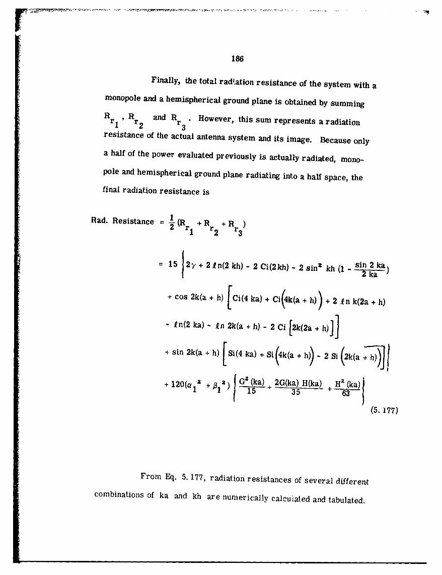
Finally, the total radiation resistance of the system with amonopole and a hemispherical ground plane is obtained by summingRrl I Rr2 and Rr3 However, this sum represents a radiationresistance of the actual antenna system and its image. Because onlya half of the power evaluated previously is actually radiated, mono-pole and hemispherical ground plane radiating into a half space, the

final radiation resistance is

Rad. Resistance = - (R + R +R2 r I r 2 r3

1 +r2 +R3)

= 15 127 +2.n(2kh)-2Ci(2kh)-2sin2kh(l sin 2 kaI f2 ka)

+ cos 2k(a + h) [Ci(4 ka) + Ci(4k(a + h) + 2 In k(2a + h)

- In(2 ka) - In 2k(a + h) - 2 Ci [2k(2a + h)]1

" sin 2k(a + h) [Si (4 ka) + Si (4k (a + h)) - 2 Si (2k(a +7)i" 120(a 1a + G2 (ka) + 2G(ka) H(ka) H2 ka) (

(5.177)

From Eq. 5. 177, radiation resistances of several differentcombinations of ka and kh are numerically calculated and tabulated.

187

The result of numerical evaluation of Eq. 5. 177 is given in

a ,raph;-al form in Fig. 5. 11, where radiation resistance is plotted as

a function of frequency. Each curve represents a different size of semi-

spherical ground plane. When the radius of a ground plane is zero,

the resulting radiation resistance corresponds to that of a monopole on

an infinite ground plane.

Results shown in Fig. 5. 11 indicates that there exists

definitely a peaking effect on the radiation resistance as the radius

of the ground plane is changed. Comparing with the monopole resonating

at 30 MHz over an infinite ground plane the radiation resistance becomes

larger with a semi-spherical ground plane well below the resonant

frequency. The peaking seems to occur at ka = 1 and this conclusion

has been drawn mainly from the results of numericai calculations.

Fig. 5. 12 and 5. 13 compare these theoretical results with

experimentally obtained input resistances. Of course, we are not

comparing the same resistances, namely the radiation resistances.

However, assuming that the loss is small, the input resistance should

be similar to the radiation resistances. Some of the discrepancies

shown in this comparison can also be explained with the discrepancies

in the assumed current and the actual current on the antenna. However,

the peaking effect is shown to exist using a small semi-spherical ground

plane with a monopole.

188

11

2a = 0 meter

... . . 2..5 i100 3.75 i

. .. . .5. 0 itC . 25 it

801h = /4 at 30 MI~z

60.)

=U6~ 2.5mr

. 40..

1 10 15 20 25 30

Frequency (MHz)

Fig. 5. 11. Theoretical radiation resistances for variousvalues of ground plane size

,.-.. - .- - P I P

189

Resistive Compoew.n of----- input impedance

(experimental)

100-__ Radiation Resistance

(Theoretical)

80-

ka =3r,/8 at 30MH;

40

ci,

5 10 15 20 26 30

Frequency (MHz)

Fig. 5. 12. Theoretical radiation resistance and experimentalinput resistance for a monopole with a hemisphericalground plane

190

Resistive Component ofinput impedance(experimental)

10C

Radiation Resistance(Theoretical)

80-

ka = r/2 at 30 MHz

60Cu

40-

20

20 "- _

5 10 15 20 25 30

Frequency (MHz)

Fig. 5. 13. Theoretical radiation resistance and experimentalinput resistance for a monopole with a hemisphericalground plane

191

Since radiation resistance is defined as the ratio of radiated

power to a square of the input current at the terminal where it is mea-

sured, the current must be that current at the terminal and resulting

cadiation resistance will be the radiation resistance at that point.

At the beginning of the theoretical analysis for this problem,

it was assumed that the current distribution on the antenna itself is in

the sinu.;oidal form.

From Eq. 5. 59, the current on the antenna is given as

I(z) = I sin k(d - z)max

where at z a, ,ink(d- z) = 1 at 30 MHz.

ThereU;'e, the input currents at the base of the antenna

(z = a) would be diff!?reni from I for frequencies lower than 30 MHz.max

We must use these cturvents to evaluate the radiation resistance at the

input terminal for each ; r qv ency.

It seems as though orte .:an have a radiation resistance as

large as desired by making the feedpoint located at a point where current

is approximately zero. One examole would be a full wave dipole which

has a zero input current at the center of the dipole. Theoretically,

then, it has an infinitely large ra( iation resistance. However, in

practice an actual antenna is not iifinitesimally thin, which was the

assumption used for deriving a (neoretical result, and the current at

a minimum point is not zero. Nevertheless, the radiation resistance

192

at a current minimum may in practice be very large, possibly

thousands of ohms.

In view of the above argument, the radiation resistance

cannot be used as a sole measure of an antenna performance. The

reactive component of an input impedance is another factor which should

be considered. When an input current is fixed at a certain value, both

the resistive and reactive components of the input impedance determine

the voltage required to maintain the current. Therefore, it is necessary

to consider a ratio of reactive component and resistive components,

or the Q of the antenna in order to decide whether increases in radiation

resistance actually increase the antenna efficiency. Input current and

voltage determines the input power and radiation resistance determines

the radiated power. The ratio of these quantities determines the efficiency

of the antenna.

In addition to the efficiency considerations, the Q of the

antenna system determines broadband tuning possibilities of the antenna.

When the antenna is electrically short, in particular, the reactive

component is usually very large and the resistive component is very

small giving very high Q values. When the reactive component is large,

a wideband tuning becomes very difficult, because one has to find a

way for a wide range variation in the conjugate reactive component to

cancel out the large radiative reactances. Also, a small value of resistive

component will cause a difficulty in transforming up to a characteristic

impedance of transmission lines normally available.

193

The ratio of a capacitive reactance to a resistance of the

antenna is defined as Q, for a monopole above an infinite ground

planc, Q of the antenna increases rapidly as frequencies go down

below resonance. Typically, for a monopole one quarter wavelength

long at 30 MHz, with the antenna or diameter ratio of approximately

400, Q at 5MHz becomes 1400 and gradually reduces to 0 at 30MHz.

The resistive component increases from 2 ohms at 5 MHz to 36 ohms

at 30Mhz. However, from the experimentally obtained data, Q of

a monopole one quarter wavelength long at 30 MHz placed above

a finite circular disc ground plane of 2. 5 meters in diameter which

is placed 1. 25 meters above an infinite natural ground is shown to

vary between 43 to 0. It is mainly due to smaller reactive components

and large resistive components over the frequency range of SMHz

through 30MHz for a monopole over a finite ground plane.

The resistive component of the input impedance contains

loss due to several sources in addition to radiation resistance. In

order to make an educated judgment on the variation of the resistive

component as a function of frequency whether it can be attributed to

an increase in radiation resistance or not, a theoretical result of

a radiation resistance for a mon )ole over semi- spherical ground

planes has been obtained. Using these theoretical results of radiation,

resistance and the experimentally obtained reactive components, Q

of the antenna has been obtained between 5MHz and 30MHz. It shows

194

that the Q of the antenna varies between 25 to 1 with X atc

10Mtz of 850 ohms compared with 900 ohms for a monopole above

an infinite ground plane.

A conclusion can be drawn from the above studies that

by using a monopole with a finite ground plane above an infinitely

large ground plane, a significant advantage can be realized in rad-

iation resistance as well as a broad band matching at the input terminals.

Through this study, a qualitative conclusion of an antenna behavior

with two ground planes has been possible. However, an exact

behavior of a monopole with a disc ground plane above an infinite

ground can only be predicted with a new mathematical model.

CHAPTER VI

CONCLUSIONS AND RECOMMENDATIONS

6. 1 ConclusionOne of the major objectives of this study was to determine

how a finite ground plane used in addition to an infinite lossly ground

affects perfornu nce of a monopole antenna. Attention was mainly

directed toward the effect of ground planes equal to, or smaller than,

a half wavelength in diameter. If there is tobe any advantage in

using these finite ground planes, they cannot be physically bulky. At

frequencies 5MHz to 30 MHz, where the study was performed, a half

wavelength at the upper end of the frequency band is equal to 5 meters.

In studying this antenna system, the length of monopole

was fi,,ed at 2. 5 meters, which is a quarter wavelength at 30 MHz.

Impedance measurements show that the real part is a strong function

of both the ground plane diameter and its location. Also it shows a

peaking effect at particular frequencies, which depends upon the

diameter of the ground plane and its location above the infinite ground.

Using a theoretical model with hemispherical ground

planes suostituted for flat discs, it was established that the sharp

increase in resistive component was largely due to an increase in radia-

tion resistance. From the theory, it seems that at least one peak

exists at frequencies where ka - 1. It was not possible to draw a

clear conclusion of this nature for an antenna with a finite disc ground

195

196

plane. When ka = 1, the distance from the base of the antenna to an

infinite ground a .ang the path of the spherical surface is a quarter

wavelength. This provides a voltage maximum or current minimum

point at the base of the antenna, regarding the infinite ground plane

as a zero potential surface. Therefore, a larger input impedance or

larger resistive component is realized at ka = 1. However, based

on the experimental results, a general conclusion that a peaking effect

occurs at frequencies approximately determined by kkP + a C where

DC is a function of the ratio -:a. It can also be concluded that the Q

of the antenna is generally mu::h lower than that of the same antenna

over an infinite ground plane, providing some advantage in designing

a tuning network at frequencies well below resonance.

Curves showing the input reactance with a finite disc-

ground plane of various sizes exhibit a region where the reactance

variation as a function of frequency is remarkably small. This

phenomenon is usually associated with a resistive maximum. Clearly,

this type of frequency response is very much better, from the point

of view of broad-band operation, than the response of either a half-

wave or a full-wave dipole. With an appropriately designed reactive

matching network the standing wave ratio on a line terminated in

the antenna with a finite ground plane over an infinite ground can be

minimized over a wide frequency range.

Because of the assumption made in the theoretical studies

that the current distribution on the monopole is in sinusoidal form

197

and independent of the surface current on the ground plane, actual

current measurements were performed using scale models. Current

distribution at the higher end of the frequency band approximated

closely the initial assumption of a sinusoidal distribution. However,

as frequency is decreased, particularly for the monopole with a hemi-

spherical ground, the actual current deviates appreciably from the

original assumption. At the lower end of the frequency band, the

current measurement shows almost a constant amplitude similar to

Hertzian dipole.

The theoretical results obtained here for the radiation

resistance assumed that the current distribution had a triangular

form at low frequencies. These results would be improved by

assumption, in the theory, of a current distrioution more closely

approximating that observed experimentally. This effect is much

more noticeable at the lower end of frequency band. Experimentally

measured input resistances confirm these facts. In Chapter 5, a

comparison is made between the theoretical and experimental radia-

tion and input resistances. The experimental values are always

larger than the theoretical values.

From the results of a theoretical study using a hemi-

spherical ground plane and the experimental results obtained for a

monopole with a finite disc ground plane above an infinite natural

ground, it can be concluded that a marked increase in radiation

resistance results with a finite disc ground plane, below the resonant

198

frequency.

The major effect of the finite ground plane upon the antenna

radiation pattern is an emergence of side lobes when the ground plane

diameter becomes appreciable compared with a wavelength. In general,

the appearance of a side lobe is not desirable, because the

power radiated is actually deviated from the main lobe where it should

be concentrated. Also the beam width measured between 3db points

from the position of the maximum amplitude is generally broader

than that of an antenna on an infinite ground plane. Theoretically, it

has been found that a spherical surface current makes only a very

slight contribution to the far-zone electromagnetic fie!d.

In summarizing the results of thL; study, it is concluded

that definitely improved performance can be obtained with an electri-

cally-short monopole antenna by operating it with a physically small

finite ground plane above natural ground. This improvement occurs

in the radiation resistance and with respect to matching network

design for a broad-band operation. These results have bearing on

the design of short monopole antennas for operation of ground-

based vehicles, in which case the antenna may be considered to be

mounted on a small ground plane above natural ground.

6. 2 Recominendation for Future Work

First, in the analysis of this problem, the infinite ground

below the finite hemispherical ground was assumed to be perfectly

199

conducting, permitting use of a conventional image technique for

solving the problem. The loss due to the finite conductivity of the

natural ground has also been neglected. However, in order to isolate

an exact radiation resistance from the measured impedance shown

in Chapter 2, it is necessary to take the loss due to the natural ground

into account.

Also, a new theoretical model consisting of an antenna on

a small ground plane above a larger ground plane, could possibly give

more accurate results than have been obtained here through assumption

of a hemispherical ground plane.

Second, since the current distribution measured shows

deviation from the original sinusoidal form, the measured current

may be taken as a given current distribution and may be decomposed

into Fourier Series to add an effect of each term. In this way, the

experimental result may be made to match better against theoretical

results.

Third, because the ultimate application of this analysis

is for a vehicular mounted antenna where a body of a vehicle can be

taken as an equivalent ground plane of a finite diameter, it is necessary

to study further to determine how a pa:ticular size of a vehicular body

and shape and location of the antenna correspond with an antenna on a

finite disc or semispherical ground plane above an infinite natural

gound.

Finally, a detailed study of the measured input impedance

200

given in Chapter 2 and deriving equivalent circuits for each case may

be useful for design of tuning networks for vehicular mounted antennas.

APPENDIX A

RECIPROCITY THEOREM

Let a source or a distribution of sources maintain a current

density J1 with associated electromagnetic fields E1 and H1 * A

second source maintains a current density J 2 with associated fields

2 and H " Then, according to Lorentz's reciprocal theorem:

v" (E 1 x H 2) - V" (E2 xH 1) = Jl" E2 "J 2 -"I (A. 1)

Let's assume that the two sets of fields are defined in free

space and are bounded by the same geometrical surfaces. Applying

volume integration on both sides of Eq. A. 1 with dV as volume element,

the integration performed over a volume V in empty space that is

bounded by a closed surface S can be written as

fff v E 1 F 2 x dv = fff v . (2 xBY dV (A. 2)V V

where

fff(Jl" E2-2 '2 E1) dV = 0 (A.3)

because all volume densities of current vanish in empty space.

From the divergence theorem

201

202

fffv (E IxHR2 ) - (E-2 x R,) dV = f ('1 1 2 E2 x F1 )' dS =0

V S

(A.4)

AWhere dS = n dS and n is an external unit normal vector

of the surface toward volume V. The only restrictions of the two setsof fields (FE , I ) and (F2' H2 ) are tint they satisfy Maxwell's equations,

the volume integration is performed in empty space V and the boundary

surfaces are in the same geometrical shape for both sets, but not neces-

sarily the same physical properties.

APPENDIX B

PROOF AND DERIVATION OF EQ. 5.56

Equation 20 was written as

Ef(x. y, Z) = ---- ff S

S (5.50)

At far-zone,

r =V(x-x')' +(y- y') 2 +(z- z') 2 -IR- R'I 5.9

can be simplified as

r~ - HRr I- RI - R

Theref ore,

e~ ekR jk -R (.5

when

203

204

Then

,N-. ikRS 'e -jkR R e -jkR= -kAVt0 R V=-jk----e R

(5.47)

where the prime notation on operator V indicates that V is operated

on the primed coordinate system.

In Eq. 5. 50, the radial component of E (x, y, z) can be

written as

ERfxf, yz - jw1L('x H) - jk(S'. R R S'

(B. 1)

Consider the following integral

1'x e- k R " R •dS = 0 (B.2)S

Where S is a closed surface bounding a volume V.

Since

Vx(Oa) = Voxa+oVxa

x (e - jk R R = V) xH e 'xH

(B. 3)

205

Therefore, Eq. B. 2 becomes

ff1 (Vx +n)e" n (Vte xH = 0S

where 4)

dS n dS

Knowing

VI-jk ' . -jkR R AVe jk e R

and

n"^ (X F) _A -R(Xx

Equation B. 4 can bc written as

ff (V' x R) e-J +" ke-A i'Jdif 3~.V~x)e~~~+R • (i x) jkeij kR R'JdS' = 0

(B. 5)Also, from Maxwell's equation

V'xH = -JWEo Exn 0 E

in a source free region.

206

Thus,

jk - -j i

• E) (-jwe 0 ) e -Jk R+ ( x H) jk e- dS'

• ~-j • dS' = 0

It is, therefore, true that

ff [ w'o% (A xR) -jk( 2 ~)eJ IdS= 0 (B. 6)

From Eq. B.1 and B.6, the radial component of E(x, y, z') is proved

to be zero at far-zone.

At far-zone, consequently,

E(x,y,z) = S n It dS (5.56)

APPENDIX C

PROOF OF EQ. 5.92

The purpose of this appendix is to show the steps involved

in arriving at Eq. 5.92 from Eqs. 5.90 and 5.91. The same steps were

also taken to get the expression (Eq. 5.106).

From Eq. 5.90 and Eq. 5.91,

2 a P (Cos O) 1n l(kR) a P (cos 0) pn (kR)

E2R U(k2 + __ )2R M (2n+ ).- k . - (ka) (2n + 1).- k .-pn (ka)

(5.90)

IIA(R) = I ma x sin k kd - R) (5.91)

where

d = a+h

Therefore,

d UaI dS 2R II()d max, f sin k(d- R)(k 2 +-L--)Pn- (kR)dRR (2n+ 1) . k. pn- 1 (ka) a aR 2

UaI d 2

max, f sin k(d- R)(k 2 + -)P n+l(kR)dR(2n+1). k'pn+ l (ka) a aR2

(C. 1)

207

208

Let

d a2=f sin k(d- R) (kz k2 da aR2 n

(C. 2)

a212 =f sin k(d RXk2 + (kR) dRa a2 n+I

Changing a variable kR to z,

kfl z .kdR dz

2 2 aaR2 a 2

The integral I I becomes

kd 2 dzI= f sin k(d -z) (k2 +k2 p C Zka az2 n ()--

kd k= k f sink(d - Z) p n- 1(z) dz + k f sink(d - z)- p n-(Z) dz (C. 3)ka ka az2 -

L,.et

kdI =k f sink(d - z) p ()dz (.4

ka n- it(.4

209

and

kd a12I k f sink(d - z)- p Wz dz (C. 5)

ka az2 -

Then

R kdI =k f sink(d-z) p n-(z) dz

kan-

Let

r n- 1(z) =u sink(d -z) dz =dv

a= z du cosk(d -z) = v

By part integration

= cosk~d z~p ( pn- 1(z)dz kI k[ cok 1 z p W- f cosk(d- Z) dzn - 1 J z = ka

Integrating the second term of 1, by part again, we get

kd ap~ n-I(Z) -f cosk(a - Z) dzka

I210U - (z n-i 1 z

=[sink(d -z) '-1 + sink(d- z) -~ (kaazz

z=ka

The second integral of the above equation is exactly the same

as I12

Rewriting 1I1 we obtain

k kd -z) pn- 1(z) + sink(d - z) p n- 1' (z)]zka 12

(C. 6)

=i 111 + 112 k [pn 1 (kd) - cos k(d - a) pn 1 (ka) - sin k(d - a) pn ka

(C. 7)

and

1 2 =k [%n+ 1 (kd) - cos k(d - a) 'r1+ l(ka) - sin k(d - a) Pn+ '(ka)j (C. 8)

211

Finally,

d U aI ~ ~ (af EI(Rc= max 7pn(kd) coskd-a)

P~~(d +co kda) P(k(ka)

Pn+ j'(k) Pn + ' (ka) (.2

APPENDIX D

NUMERICAL EVALUATION OF Bn

The functions shown in the evaluation of the coefficients Bn

of an infinite series expressing an induced surface current on a hemi-

spherical ground plane are the weighted spherical Hankel functions of

the second kind andtheir derivatives.

These functions p n (x) crn be expressed in the form of a

series such as

X W = xh(2)( (J)n+le- n (n+ 'k ) 1 (D. )

k=o (2j x)

where

+ k) (n + k)!2 k! P(n -k +_1)

rJ(z+1) = z! z: integers

h(2)(x) = Hn1 (2) (x) and j = I2

Also, from the recurrence relations of Hankel functions, the

following relationship between the spherical Hankel functions and their

derivatives can be obtained (Ref. 18 ).

212

213

h(2)(x) (2) n+ (D.)d- n x n

and

dp n() = d (x h (2)(x)) = h (2 )(x) + x -L~ h (2 )(x) (D. 3)

From Eqs. D. 2 and D. 3, the following relationships are

derived

#o() dx o0d Po(X) (2Po (x) - dx --h= ) x h (() (.4

d n(X) - (x)- nh (2x) (D. 5)Pn~x( x d x h n-I x n

pn(x) xh n (x) (D. 6)

Equations D. 4, D. 5, and D. 6 are used with a table for spheri-

cal Hankel functions to evaluate the coefficients Bn

APP ,NDIX E

EVALUATION OF R r in Eq. 5.168

From the power series representation of cosine integral

Ci(z), Eq. 5. 165, the terms associated with cosine integral of a small

arguient can be written as

lini Ci(2k(a + h) e y + In 2k(a + h) + lim In(c) (E.1)E-0 E-O

lim Ci(2ka E) y + fn(2ka) + lim In(c) (E. 2)E-0 E-0

lim Ci k(2a + h) E , + fn(k(2a + h))+ lim In(E) (E.3)E-0 E-0

lim Ci(khe) y + in(kh) + lim .n(E) (E.4)E-0 E- 0

Substituting Eq. E. 1 through Eq. E. 4 into appropriate places in through

0

R = 60 in 2- lim I n E + .+ lim I n(E) + I n(kh) - lcos 2k(a + h) I n(2ka)I E -0 E-O0

- cos 2k(a + h) in 2k(a + h) + cos 2k(a + h) kn(2a + h)k - Ci(2kh)

+ -1 cos2(a +h) Ci(4ka) + -sin 2k(a + h) Si(4ka) - (1 sin2ka ) sin 2 kh2 14 2k

214

215

-cos 2k(a + h) Ci(2k(a + h)) - sin 2k(a + h) Si(2k(2a + h))

+-cos 2k(a + h) Ci (4k(a + h) + 1 sin 2k(a + h) Si (4k(a + h)

(E. 5)

It should be noticed that the coefficients of Y and In(E)

associated with the cosine integrals add up to 1. This can be shown

easily after sMTT algebraic 'manipulation with trigonometric identities.

After cancelling out the logarithmic singularities in Eq. E. 5

and collecting termb, the final form of Eq. E. 5 can be shown as Eq. 5. 168.

216

REFERENCES

1. S. J. Bardeen, "The Diffraction of a Circularly SymmetricalElectromagnetic Wave by a Coaxial Circular Disc of FiniteConductivity, " Physical Review, Vol. 36, Nov. 1930, p. 1482.

2. G. H. Brown & 0. M. Woodward, Jr., "Experimentally DeterminedImpedance Characteristics of Cylindrical Antennas, " Proc. IRE,April 1945, p. 257.

3. A. Leitner & R. D. Spence, "Effect of a Circular Ground Planeon Antenna Radiation, " J. Appl. Phys., Vol. 21, Oct. 1950,p. 1001.

4. J. E. Storer, "The Impedance of an Antenna Over a Large CircularScreen, "J. Appl.. Phys., Vol. 22, No. 8, Aug. 1951, p. 1058.

5. C. L. Tang, "On the Radiation Pattern of a Base-Driven AntennaOver a Circular Conducting Screen, " J. Soc. Indust. Appl. Math.Vol. 10, No. 4, Dec. 1962, p. 695.

6. J. R. Wait & W. A. Pope, "Input Resistance of L. F. UnipoleAerialsc" Wireless Engineers, May 1955, p. 131.

7. G. H. Brown, R. F. Lewis, & J. Epstein, "Ground Systems asa Factor in Antenna Efficiency, " Proc. IRE, Vol. 25, 1937, p. 753.

8. F. R. Abbot, "Design of Buried R. F. Ground Systems," Proc. IRE,Vol. 40, 1952, p. 846.

9. R. King & C. W. Harrison, "The Distribution of Current Along aSymmetrical Center-Driven Antenna, " Proc. IRE; Oct. 1943, p. 548.

10. H. Whiteside & R. King, "The Loop Antenna as a Probe, " IEEE Trans.Antennas & Propagation, Vol. AP- 12, May 1964, p. 291.

11. H. Jasik (Editor), Antenna Engineering Handbook McGraw.-HillBook Co., Inc., New York, 1961.

12. R. W. King, Fundamental Electromagnetic Theory. Dover Publication,Inc., New York, 1963.

217

REFERENCES (CONT.)

13. J. E. Storer, "Impedance of Thin Wire Loop Antennas," Trans.AIEE (Comm. and Electronics), November 1956, p. 606.

14. .1. A. Stratton, Electromagnetic Theory, McGraw-Hill Book Co.,Inc., New York, 1941.

15. 0. Norgorden & A. W. Walters, "Experimentally DeterminedCharacteristics of Cylindrical Sleeve Antennas," J. Am. Naval Engrs.,May 1950, p. 365.

16. C. H. Papas & R. King, "Surface Currents on a Conducting SphereExcited by a Dipole," J. Appl. Phys., Vol. 19, Sept. 1948, p. 808.

17. W. Magnus & F. Oberhettinger, Formulas and Theorems for theFunctions of Mathematical Physics, Chelsea Publishing Co., NewYork, 1954.

18. M. Abramowitz & I. Stegun (Editors), Handbook of MathematicalFunctions With Formulas t Graphs, and Mathematical Tables, NBSApplied Math. Series 55, June 1964.

Date post:	14-Jun-2018
Category:	Documents
Upload:	hoangdien
View:	218 times
Download:	0 times

DISTRIBUTED BY: National Technical Information … · TOTAL NO OF P.GEv Tb NO 1)F pEPr$ ... or...

Documents