Distributed Coordination Strategies for

Wide-Area Patrol

Brandon J. Moore and Kevin M. Passino∗

Dept. Electrical and Computer Engineering

The Ohio State University

Columbus, OH 43210

mooreb@ece.osu.edu, passino@ece.osu.edu

May 25, 2006

Abstract

This paper addresses the problem of enabling a group of autonomous vehicles to effectively patrol an

environment significantly larger than their communication and sensing radii. The environment is divided

into smaller areas and special coordinator vehicles are designated to control the transfer of the other

vehicles from one area to another. Our past work showed that by organizing the areas and coordinators

into a ring topology, we could design a control algorithm that globally balanced the number of vehicles

in all areas within a bounded length of time. This paper extends those results to a much broader class of

area-coordinator topologies and this added flexibility can be used in implementation to reduce the time

it takes to attain the globally balanced state.

1 Introduction

This work is motivated by a mission scenario first proposed in [1] in which a group of autonomous vehicles

with range-limited communications and sensing is tasked to cooperatively patrol a relatively large environ-

ment (i.e., an environment whose dimensions dramatically exceed the vehicles’ maximum communication

and sensing radii). The limited communication and sensing radii mean that the vehicles must reach a com-

promise between distributing themselves throughout the environment (to reduce gaps in patrol coverage)

and maintaining some cohesion as a group (because they will need to communicate at least periodically in∗This work was supported by the AFRL/VA and AFOSR Collaborative Center of Control Science (Grant F33615-01-2-3154).

1

order to cooperate with each other). Because of space constraints we will proceed directly to our problem

formulation and refer the reader to [1] for a full description of this scenario and the technological justifications

for the restrictions on communications and sensing.

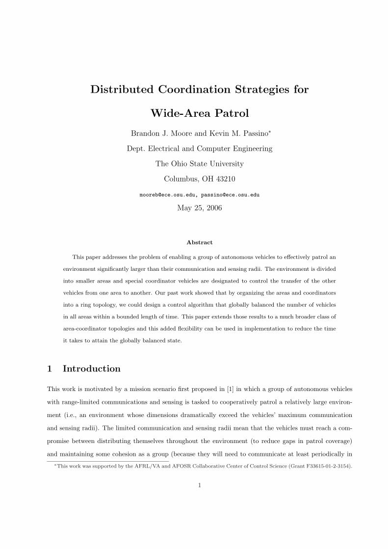
The approach to this problem we took in [1] is as follows. The environment was first broken down into a

number of smaller areas to which individual vehicles could be assigned (see Figure 1). The idea behind this

spatial decomposition was that by restricting a vehicle to a small section of the environment, it should be

easier to determine how that vehicle should behave in order to efficiently patrol that area. More specifically,

if there are one or more locations in an area to which a vehicle can go to in order to communicate with

another vehicle, then the small size of that area means that a vehicle can patrol a significant portion of

that area in between visits to those locations and still communicate on a fairly regular schedule. That is

to say that a vehicle can spend most of its time actually patrolling the area and still remain connected to

the group through periodic communication. Of course, in order for a vehicle to communicate by going to

one of these special locations, there must be another vehicle there. This brings us to the second part of our

approach which was the establishment of a number of coordinators. Coordinators are simply a small number

of the group’s vehicles that remain along the boarder between two or more areas and provide the previously

mentioned locations where the other vehicles can come to communicate. Exactly how the coordinators and

the patrol vehicles can meet up to communicate is highly dependent on the nature of the vehicles and the

specifics of the scenario and we direct the reader to [1] for more discussion on this topic.

patrol area

nominal coordinator

locations

vehicle

communication

zones

Figure 1: A simple four-area example.

The preceding formulation of the problem into areas and coordinators breaks the group of vehicles into

a two-level hierarchy. At the bottom level we have the majority of the vehicles, and from this point on we

will simply use “vehicle” and “vehicles” to refer to these members of the group. Being confined to one area

at a time, the vehicles’ main job is simply to gather information from that limited region and report it back

to the coordinators. Forming the upper level, the coordinators are responsible for collecting the information

from the vehicles and passing it on (e.g., via the vehicles) to other coordinators and potentially a human

operator, directing the vehicles’ efforts within the area (i.e., telling them where to go look if a certain part of

2

the area has something interesting in it or has not been observed for a while), and, most importantly, shifting

vehicles between the areas they oversee (i.e., the ones they “connect” by virtue of their nominal location) in

order to achieve the proper distribution of vehicles across all the areas. For now we will consider the proper

distribution of vehicles to be one in which the number of vehicles in each area is globally balanced. By this we

mean that the number of vehicles in any area differs from that of any other area by no more than one. The

reasoning behind our desire for a globally balanced distribution is that unless we have specific information

that leads us to believe it is better to concentrate more vehicles in certain regions, we want to spread them

out as uniformly as possible across the environment to reduce the gaps in coverage. When the areas are all

the same size (as would be the case with a regular gridding of the environment), then this corresponds to

wanting the number of vehicles in each area to be as equal as possible (and unless the number of vehicles is

evenly divisible by the number of areas, then the best we can do is to have any two areas differ by no more

than one vehicle). Of course, in some cases it will be desirable to be able to specify a weighted balancing of

the vehicles (i.e., when we want each area to have a proportion of group’s vehicles that is equal to its relative

priority).

Other work in cooperative control that shares some similarities with our scenario include those that

deal with “pop-up” targets [2, 3] and those that deal with the spatial allocation of resources [4]. However,

the most closely related work to ours is that concerning load balancing in distributed computing [5, 6, 7].

Our problem differs in that multiple coordinators will have control over any given area (as opposed to a

single processor having control over its task load) and since we demand a globally balanced distribution (as

opposed to a locally balanced distribution in which only neighboring processors are balanced to within one

load block). The issue of achieving a globally balanced distribution has received only limited attention in

the literature prior to [1]. Improvements on local balancing have been achieved both with message passing

[8] and non-deterministic algorithms [9], but neither of these guarantees global balancing. The algorithm

presented in [10], which shares some commonalities with [1], does achieve a globally balanced distribution

but is specific to applications involving a grid of parallel processors and does not address the information

delays or asynchronism present in our scenario.

2 Global Balancing on a General Topology

2.1 Overview of Dynamics and Results

In order to better explain our work, we provide a high level overview of how we are able to achieve our results

in this section before getting into the more technical description in the sections that follow. As stated, this

3

work is an extension of [1] which used a ring interconnection in which vehicles could only be transferred in

one direction. While it does achieve global balancing, this unidirectional ring setup has the disadvantage

of taking a considerable amount of time to converge to the globally balanced state in some circumstances.

For example, if all the vehicles in the system initially start out in one area, then in order to put a vehicle

in the area just preceding that area in the ring a vehicle has to be sent all the way around the ring (even

though that area lies right next to that area physically). The purpose of this paper, then, is to extend the

results of [1] to a less restrictive class of topologies. In order to do this we have changed the basic unit of

the system from an area to a sub-area. That is to say that a vehicle will not just be assigned to an area, but

also assigned to a sub-area within that area. We emphasize that we have chosen the term “sub-area” for the

way it will help us to visualize the system’s structure and the distributed coordination scheme and that this

choice is in no way meant to reflect a physical partition of the areas (i.e. the vehicle assigned to a sub-area

can still patrol anywhere in the area to which that sub-area belongs). Just as the areas are connected into

unidirectional ring, so are the sub-areas (and the sub-area ring follows the area ring). However, in addition

to being able to transfer resources along this ring, the coordinators will also be able to transfer vehicles

across “shortcuts” to this ring (details as to how these shortcuts are established are given in Section 2.2

below). The effect of these shortcuts is to dramatically reduce the number of areas that a vehicle will have

to traverse in order to get to where it is needed.

The essential dynamics of the sub-area ring in this paper are the same as those for the area ring of [1],

although the presence of the shortcuts can result in much more complicated behavior and as a consequence,

the control algorithm discussed in Section 2.4 will have to much more complex than that of [1] in order to

ensure that we can still achieve the globally balanced state. In order to help the reader better understand

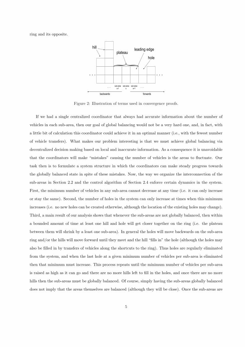
these dynamics we introduce the visualization aid shown in Figure 2. In this figure, each sub-area in the ring

is drawn as a stack of identically sized blocks, with the number of blocks in this stack equal to the number

of vehicles in that area. These sub-area stacks are arranged according to the order specified by the sub-area

ring with the stack for a sub-area drawn to the left of the stack for the next sub-area in the ring and to the

right of the stack for the preceding sub-area. (The sub-area ring eventually wraps back upon itself, but only

a section of the ring is drawn in Figure 2). The low spots in this picture correspond to the sub-areas with

the smallest number of vehicles and we call these areas holes. The relatively high spots (sub-areas that have

at least two more vehicles than the hole areas) we call hills. In between are those areas that have exactly

one vehicle more than the hole areas and we call a group of these areas in sequence a plateau (and we will

sometimes refer to the sub-area in a plateau that is most advanced along the ring as its leading edge). The

directions forward and backward refer respectively to the direction that vehicles may be passed around the

4

ring and its opposite.

...

hill

plateau

hole{forwardsbackwards

sub-area

s

sub-area

s-1

sub-area

s+1......

leading edge

...

Figure 2: Illustration of terms used in convergence proofs.

If we had a single centralized coordinator that always had accurate information about the number of

vehicles in each sub-area, then our goal of global balancing would not be a very hard one, and, in fact, with

a little bit of calculation this coordinator could achieve it in an optimal manner (i.e., with the fewest number

of vehicle transfers). What makes our problem interesting is that we must achieve global balancing via

decentralized decision making based on local and inaccurate information. As a consequence it is unavoidable

that the coordinators will make “mistakes” causing the number of vehicles is the areas to fluctuate. Our

task then is to formulate a system structure in which the coordinators can make steady progress towards

the globally balanced state in spite of these mistakes. Now, the way we organize the interconnection of the

sub-areas in Section 2.2 and the control algorithm of Section 2.4 enforce certain dynamics in the system.

First, the minimum number of vehicles in any sub-area cannot decrease at any time (i.e. it can only increase

or stay the same). Second, the number of holes in the system can only increase at times when this minimum

increases (i.e. no new holes can be created otherwise, although the location of the existing holes may change).

Third, a main result of our analysis shows that whenever the sub-areas are not globally balanced, then within

a bounded amount of time at least one hill and hole will get closer together on the ring (i.e. the plateau

between them will shrink by a least one sub-area). In general the holes will move backwards on the sub-area

ring and/or the hills will move forward until they meet and the hill “fills in” the hole (although the holes may

also be filled in by transfers of vehicles along the shortcuts to the ring). Thus holes are regularly eliminated

from the system, and when the last hole at a given minimum number of vehicles per sub-area is eliminated

then that minimum must increase. This process repeats until the minimum number of vehicles per sub-area

is raised as high as it can go and there are no more hills left to fill in the holes, and once there are no more

hills then the sub-areas must be globally balanced. Of course, simply having the sub-areas globally balanced

does not imply that the areas themselves are balanced (although they will be close). Once the sub-areas are

5

balanced, however, the control algorithm in Section 2.4 will stop transferring vehicles across the shortcuts

to the sub-area ring and so the system will essentially act like the unidirectional area ring of [1] and the

areas will be globally balanced within a bounded length of time. Although this explanation of the system

dynamics seems fairly simple, we remind the reader that we are only describing a subset of the system’s

dynamics and that many other vehicles transfers are being made in addition to ones involved in the above

process. In fact, ensuring that these other transfers do not interfere with the filling in of holes is not at all

trivial and will require a very carefully designed distributed control algorithm.

2.2 Interconnection Design Requirements

In this section we describe the class of area-coordinator interconnections that will still allow us to achieve

global balancing under an (extensive) modification of the control algorithm used in [1]. Although much more

general than the unidirectional ring used before, there will still be a number of restrictions on the type of

interconnections that may belong to this class. We will see in Section 4, however, that these restrictions do

not pose much of a problem for typical scenarios.

To describe the area-coordinator interconnection, we start by letting A = {1, . . . , NA} denote the set

of NA areas and letting C = {1, . . . , NC} denote the set of NC coordinators. To lessen confusion we will

endeavor to use variants of a to denote specific areas and variants of c to denote specific coordinators. Let

A(c) be the set of areas that coordinator c connects (by virtue of its physical location) and let C(a) be the set

of coordinators connected to area a. The area-coordinator interconnection is best described by a bipartite

graph (A ∪ C, I) with vertices from A and C and a set of edges I ⊆ A × C which contains the edge (a, c) if

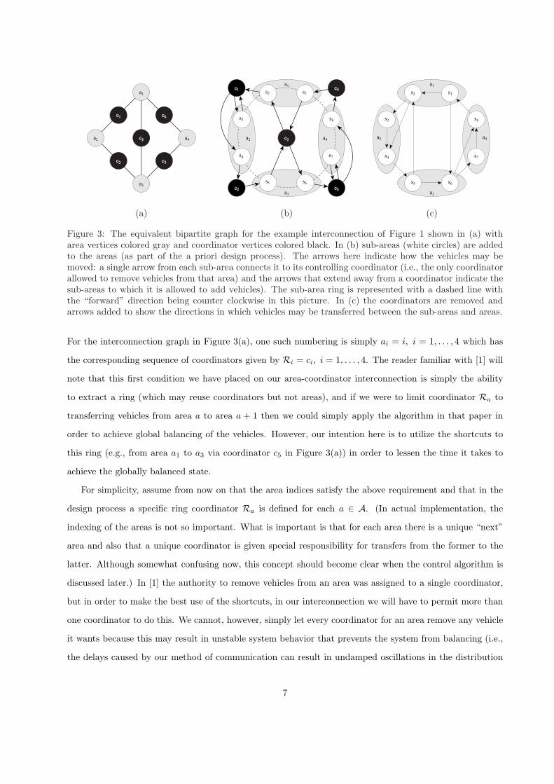
and only if a ∈ A(c) (or, equivalently, if and only if c ∈ C(a)). For a simple example consider Figure 3(a)

which shows the bipartite graph constructed from the physical layout in Figure 1.

With notation for the interconnection in hand we can now state the main requirement that the design of

our interconnection must satisfy, namely that it must be possible for a vehicle starting in any area to travel

through the interconnection (via transfer from one area to another by a connecting coordinator) in such a

manner that it visits each area once and only once before returning to its original location. To define this

technically, let us first define the addition and subtraction operations on the area indices such that their

output “wraps” into the set A so, for example, a + 1 = 1 when a = NA and a − 1 = NA when a = 1. We

can technically define this operation as a + i = mod(a + i − 1, NA) + 1, where mod(p, q) = p − qbpq c and

b·c is the floor function (i.e., the largest integer no greater than its argument). Now our restriction on the

interconnection (A∪C, I) can be stated as follows: there must exist some numbering of the areas such that for

every a ∈ A there exists a “ring” coordinatorRa that connects area a to area a+1 (i.e., Ra ∈ C(a)∩C(a+1)).

6

a1

a2 a4

a3

c1 c4

c5

c3c2

a2

s2 s1

s8s3

s4

s5 s6

s7

a1

a3

c1

c3c2

a4

c4

c5

s2 s1

s8s3

s4

s5 s6

s7

a2 a4

a1

a3

(a) (b) (c)

Figure 3: The equivalent bipartite graph for the example interconnection of Figure 1 shown in (a) witharea vertices colored gray and coordinator vertices colored black. In (b) sub-areas (white circles) are addedto the areas (as part of the a priori design process). The arrows here indicate how the vehicles may bemoved: a single arrow from each sub-area connects it to its controlling coordinator (i.e., the only coordinatorallowed to remove vehicles from that area) and the arrows that extend away from a coordinator indicate thesub-areas to which it is allowed to add vehicles). The sub-area ring is represented with a dashed line withthe “forward” direction being counter clockwise in this picture. In (c) the coordinators are removed andarrows added to show the directions in which vehicles may be transferred between the sub-areas and areas.

For the interconnection graph in Figure 3(a), one such numbering is simply ai = i, i = 1, . . . , 4 which has

the corresponding sequence of coordinators given by Ri = ci, i = 1, . . . , 4. The reader familiar with [1] will

note that this first condition we have placed on our area-coordinator interconnection is simply the ability

to extract a ring (which may reuse coordinators but not areas), and if we were to limit coordinator Ra to

transferring vehicles from area a to area a + 1 then we could simply apply the algorithm in that paper in

order to achieve global balancing of the vehicles. However, our intention here is to utilize the shortcuts to

this ring (e.g., from area a1 to a3 via coordinator c5 in Figure 3(a)) in order to lessen the time it takes to

achieve the globally balanced state.

For simplicity, assume from now on that the area indices satisfy the above requirement and that in the

design process a specific ring coordinator Ra is defined for each a ∈ A. (In actual implementation, the

indexing of the areas is not so important. What is important is that for each area there is a unique “next”

area and also that a unique coordinator is given special responsibility for transfers from the former to the

latter. Although somewhat confusing now, this concept should become clear when the control algorithm is

discussed later.) In [1] the authority to remove vehicles from an area was assigned to a single coordinator,

but in order to make the best use of the shortcuts, in our interconnection we will have to permit more than

one coordinator to do this. We cannot, however, simply let every coordinator for an area remove any vehicle

it wants because this may result in unstable system behavior that prevents the system from balancing (i.e.,

the delays caused by our method of communication can result in undamped oscillations in the distribution

7

of vehicles).

The approach we use for distributed coordination is to add another level of organization to the system.

Instead of being directly assigned to an area, each vehicle will be assigned to a sub-area within a specific

area. Specifically, let us define a set of NS sub-areas as S = {1, . . . , NS}, and let A(s) be the area to which

sub-area s belongs. In addition, each sub-area s will be “owned” by a coordinator C(s), where C(s) must

be one of the coordinators connected to area A(s) in our interconnection. (We note that for the purpose of

convenience we are using a slight abuse of notation here by letting the functions C(·) and A(·) depend on

their argument’s type.) In our distributed coordinator strategy, to say that a coordinator owns a sub-area

will imply that that coordinator has the sole authority to remove vehicles from that sub-area. Before we

continue, we again emphasize that we have chosen the term “sub-area” for the way it will help us to visualize

the system’s structure and the distributed coordination scheme and that this does not imply a physical

partition of the areas. On the contrary, a vehicle in sub-area s can still be tasked to patrol anywhere with

the physical limits of area A(s) and will still check in with the other coordinators for that area.

The purpose of the sub-areas is to provide a structure that facilitates the control algorithm presented

later, and so there will be number of rules that govern the way this sub-area structure is designed. Before we

get to these rules, let us first define the set S(a) to be the sub-areas of area a and let the set S(c) to be the

sub-areas owned by coordinator c. For convenience let us also define a constant pa = |S(a)| to be the number

of sub-areas in area a. Now our first rule, which we have already mentioned above, is that the coordinator

for a sub-area must also be a coordinator for the area to which that sub-area belongs (i.e., C(s) ∈ C(A(s))

for all s ∈ S). If this were not the case then we would have a situation in which a coordinator which did

not connect to an area was responsible for some of the vehicles in that area. Our second rule is that there

must be at least one sub-area in each area (i.e., pa ≥ 1 for all a ∈ A) which is necessary since we need

the capability to assign vehicles to any area. Now, letting the addition and subtraction operations on the

sub-area indices be defined in a similar manner to those for the area indices (i.e. the result of s + i wraps

into S), our third rule is that the indices of the sub-areas must be chosen such that a vehicle repeatedly

transferred from sub-area s to sub-area s + 1 will visit each area in the ring defined by the area indices once

and only once. This condition essentially states that the sub-areas’ indices define a sub-area ring that follows

the established area ring. Stated more precisely, it must be the case that (i) all the sub-areas within an area

must have consecutive indices (e.g., in Figure 3(c) both s1 = 3, s2 = 4 and s1 = 8, s2 = 1 are legitimate) and

(ii) for every area a there exists a unique sub-area ra ∈ S(a) such that ra + 1 ∈ S(a + 1) and C(ra) = Ra

(i.e. sub-area ra is the last sub-area in area a and the sub-area that follows it in the sub-area ring is in area

a + 1 and, in addition, it must be that sub-area ra is owned by coordinator Ra). For example s2 = 4, s3 = 5

8

in Figure 3(c) is legitimate because the coordinator for s2 connects areas a1 and a2). Again, we note that

in implementation the actual indices of the sub-areas are not important so long as the coordinator for a

sub-area s knows which sub-area comes next in the sub-area ring.

With the structure discussed above in place we can now discuss the manner in which vehicles may be

transferred from one sub-area to another. In [11] we used an almost identical setup and for each sub-area

s we allowed coordinator C(s) to transfer a vehicle from s to any other sub-area in any area to which that

coordinator connected. This is the most permissive option, and although it works in the perfect information

case of [11] we run into a number of problems when delays in information are introduced that do not permit

global balancing of either the sub-areas or areas (e.g., new holes can be created and the minimum number

of vehicles per sub-area may actually decrease). Thus, for this work we will restrict the set of sub-areas to

which a coordinator may transfer vehicles. We already have that S(c) is the set of sub-areas from which

coordinator c may remove vehicles (i.e., a set of “source” sub-areas for coordinator c), so let us define a

set D(c) as the set of sub-area to which coordinator c may transfer vehicles (i.e., a set of “destination”

sub-areas for coordinator c). Specifically, D(c) will consist of all sub-areas s ∈ S for which coordinator c is

associated with sub-area s − 1 (i.e., s ∈ S(c) ⇔ s + 1 ∈ D(c)). Seen from another perspective, we say that

only coordinator C(s− 1) can add vehicles to sub-area s. For an example of how this works see Figure 3(b).

In this diagram the sub-area ring has been denoted by a dashed line and sub-area s2 follows sub-area s1,

etc. Coordinator c5 has been associated with sub-areas s1 and s5 so it may remove vehicles from either of

these two sub-areas and transfer them to either sub-area s2 or sub-area s6. The reason we have chosen to

limit vehicle transfers in this way is that it preserves a relationship where for every sub-area exactly one

coordinator may remove vehicles and exactly one may add vehicles. In [1] this relationship resulted in very

useful properties that allowed us to achieve global balancing. In contrast to [1] where each coordinator was

limited to transferring vehicles from just one area to the next, our present formulation allows coordinators to

transfer vehicles to multiple sub-areas and allows us to utilize the shortcuts to the area ring in order to get

faster balancing (e.g., Figure 3(c) illustrates how the shortcut between areas a1 and a3 is preserved). One

thing we should point out (and is illustrated in Figure 3(b)) is that it is not necessary for a coordinator c

to have a sub-area in every area to which it may transfer vehicles (see coordinators c2 and c4). Specifically,

coordinator Ra does not have to have a sub-area in area a+1 in order to transfer vehicles to a+1 because it

may transfer vehicles to sub-area ra+1 ∈ S(a+1) by virtue of being the coordinator associated with sub-area

ra. In general, of course, if a coordinator does not have a sub-area in a certain area then it is effectively

disconnected from that area. Another thing to note is that we have not limited the number of sub-areas

that may be associated with a given coordinator, so a coordinator may have more than one sub-area in an

9

area (a flexibility that will be useful when we want each area to have the same number of sub-areas in each

area but every area does not have the same number of coordinators).

2.3 Estimation Methods and Properties

The fundamental feature of our distributed coordination problem that makes it interesting is that there is

significant delay between the action of one coordinator (i.e., the transfer of a vehicle from one sub-area to

another) and another coordinator’s recognition of that action. Specifically, a coordinator will not realize

that a vehicle has been added to a sub-area until that vehicle checks in with it and it will not realize that

a vehicle has been removed from a sub-area until the vehicle fails to check in for such a long time that the

coordinator can assume it has been removed. Because of this, it is generally impossible for a coordinator

to have accurate information about the number of vehicles in any particular sub-area or area. The purpose

of this section is to demonstrate how the coordinators can estimate these numbers (and other important

quantities) and explore some important properties of these estimates that will allow the coordinators to

make decisions about local vehicle transfers that will ultimately result in a globally balanced state.

Assume that we are given some length of time d which denotes the longest period of time a vehicle can go

without checking in with any specific coordinator for the area to which it is assigned (and assume this value is

known to all the coordinators). The value of d is determined by the physical layout of the area-coordinator

interconnection and the dynamics of the vehicles (e.g., their maximum speed) and must be chosen large

enough so that a vehicle can check in with all the other coordinators for its assigned area and still have

enough time left over to do some useful patrol work. Assume also that each vehicle is given an identification

number that is unique. In order to avoid confusion, we will actually require that this identification number

be reassigned every time a vehicle is transferred from one area to another (but not when transferred between

sub-areas within the same area) and that the new identification number be unique from any identification

number used in the past. This is easily implemented by having the coordinator that transferred the vehicle

into a new area give that vehicle a new number consisting of that coordinator’s index value and the date

and time (according to the coordinator’s local clock) that that vehicle was transferred. If simultaneous

transfers of vehicles are allowed, then the coordinator can either add one more field to the identification

number in order to distinguish between the vehicles or it can simply adjust the time field slightly to make

each identification number unique (e.g., by adding a small number of seconds to each time field). Now, in

order to generate an estimate for the number of vehicles in a sub-area, a coordinator will simply keep a list

of the vehicles it thinks are still assigned to that sub-area. A vehicle gets added to this list the first time it

checks in with that coordinator and removed whenever it has not visited that coordinator within a length

10

of time greater than d. Obviously whenever a coordinator transfers a vehicle it can update its list for both

the source and destination sub-areas immediately. The coordinator’s estimate of the number of vehicles in

that sub-area is then simply the length of this list, and in our system this estimate has a number of useful

properties.

Now, each coordinator c will have to maintain an estimate for each sub-area in either S(c) or D(c). One

of our fundamental assumptions in will be that no vehicles enter or leave the system for time t ≥ tinit − d,

where tinit is the initial time. This gives us two useful properties for coordinator c’s estimates of the sub-areas

in S(c) and D(c). Specifically, for any sub-area s ∈ S(c) and any time t ≥ tint, it must be the case that

coordinator c’s list of vehicles it thinks are in sub-area s differs from the true number only by those vehicles

that were added by coordinator C(s− 1) in between time t− d and t (because coordinator c = C(s) is the

only coordinator that can remove vehicles from sub-area s). Thus we have that coordinator c’s estimate for

a sub-area s ∈ S(c) can never be greater than the true number of vehicles in s. In addition, if coordinator

C(s − 1) has not added any vehicles to sub-area s from time t − d to time t, than this estimate must be

correct because every vehicle added prior to t − d will have checked in with coordinator c by time t. By a

similar argument we also have that coordinator c’s estimate for a sub-area s ∈ D(c) can never be less than

the true number of vehicles in s and if coordinator C(s) has not removed any vehicles from sub-area s from

time t− d to time t, than this estimate must be correct.

In addition to maintaining the above estimates for the sub-areas in their source and destination set,

those coordinators designated as ring coordinators must also maintain a number of other estimates due to

the special role they will play in our control algorithm. Specifically a ring coordinator for area a, Ra must

maintain an estimate for every sub-area in both area a and a + 1. With the exception of sub-areas ra and

ra + 1 (which are in S(Ra) and D(Ra) respectively), coordinator Ra is not guaranteed to have the nice

relationship between it’s estimate for a sub-area s ∈ S(a) ∪ S(a + 1) and the true number of vehicles in s

because its list for that sub-area at time t will generally contain some vehicles that have been removed by

coordinator C(s) (but whose absence has not yet been detected by coordinator Ra) and will also be missing

some vehicles that have been added by coordinator C(s− 1) (but have not yet checked in with coordinator

Ra). Under special circumstances, however, these estimates may satisfy certain properties. Specifically, for

any sub-area s ∈ S(a)∪S(a + 1) if coordinator C(s) has not removed any vehicles from s from time t− d to

t, then coordinator Ra’s estimate for s must be no greater than the true number of vehicles in that sub-area.

Conversely, if coordinator C(s − 1) has not added any vehicles to s from time t − d to t, then coordinator

Ra’s estimate for s must be no less than the true number of vehicles in that sub-area.

The ring coordinators will also have to maintain estimates of the total number of vehicles in areas a and

11

a+1. This can be done simply by adding the estimates for the individual sub-areas in S(a) or S(a+1), and

the way the coordinators’ keep their lists for these sub-areas gives us a couple of nice properties for these

area estimates. We first note that since a vehicle’s identification number changes only in inter-area transfers,

whenever a coordinator notes that a vehicle it thought was in sub-area s ∈ S(a) is now in sub-area s′ ∈ S(a),

it can update both lists simultaneously. In other words, the recognition of this intra-area vehicle transfer

does not affect the coordinator’s estimate for a. As a direct implication of the properties for Ra’s sub-area

estimates discussed above, whenever coordinator Ra is the only coordinator to remove vehicles from area

a from time t − d to time t, then Ra’s estimate for area a can be no greater than the true number. In

addition, if none of the other coordinators for area a have added vehicles to that area during the same time

frame, then coordinator Ra’s estimate for a must be correct. Conversely, whenever coordinator Ra is the

only coordinator to add vehicles to area a + 1 from time t − d to time t, then Ra’s estimate for area a + 1

can be no less than the true number, and if none of the other coordinators for area a have removed vehicles

from that area during the same time frame, then coordinator Ra’s estimate for a + 1 must be correct.

2.4 Basic Model of Distributed Dynamics

To model our system, we will use a discrete event system (DES) model of the type described in [12]. This is

a partially asynchronous model [5] in which the state of the system is updated according to the occurrence

of certain events, with the current state of the system and certain assumptions about the system’s behavior

governing which events may occur at any given time. We start by defining our state variables, all of which

take values in the set of non-negative integers N = {0, 1, 2, . . .}. The number of vehicles in sub-area s will

be denoted by xs and a coordinator c’s estimate of that number will be denoted by xcs (and for a particular

sub-area s this variable is only defined for a coordinator c if c owns sub-area s and/or owns sub-area s− 1

and/or is the ring coordinator for either area A(s) and/or A(s) − 1). Let x be the complete state of the

system (i.e., the collection of the above xs and xcs values defined for each s ∈ S and applicable values of c)

and let X = N|x| be the state space. For notational convenience, let us define xRa as the vector containing

ring coordinator Ra’s estimates of the sub-areas in areas a and a + 1 (i.e., xRa = [xRara−pa+1, . . . , x

Rara+1

]>).

Also for convenience, let us define the functions ya =∑

s∈S(a) xs and yca =

∑s∈S(a) xc

s to be the total number

of vehicles in area a and coordinator c’s perception thereof (defined only for c ∈ Ra∪Ra−1). Let x(k) denote

the state of the system at time step k ∈ N, where k maps to a real time value t(k) and this mapping satisfies

t(k′) > t(k) whenever k′ > k.

As mentioned, the state of the system is altered by the occurrence of particular events. Let us denote the

set of all events that occur at time step k as e(k). The set e(k) contains one or more “partial” events that

12

describe changes to the system such as the transfer vehicles from one sub-area to another and a coordinator

updating its various estimate values. Let eαs→s? denote the transfer of α vehicles from sub-area s to sub-area

s?. Let e+βc,s denote an increase of β to coordinator c’s estimate for sub-area s occurring when c adds a new

vehicle to its list for s and let e−γc,s denote a decrease of γ to that estimate occurring when a vehicle on that

list misses its check-in deadline and is removed. With these definitions we can also denote the set to which

an event e(k) must belong as the event space E . Simply speaking, an element of E is any collection of partial

events that are each properly defined (i.e., α, β, and γ must always be non-negative integers, s? must be in

D(C(s)) for transfer events, and c and s must correspond to a state variable xcs for estimate change events).

With the above description of our event space, we can easily define the update to the state that occurs at

each time step as follows. First, the state xs(k + 1) is equal to xs(k) plus the net transfer of vehicles in and

out of sub-area s at time step k. Second, the estimate xcs(k + 1) is equal to xc

s(k + 1) plus all the increases

and minus all the decreases that occur at time step k.

Now, while the event space E lists all the possible events that could theoretically occur, the physical

behavior of our system will greatly curtail both the number of events that may occur at a particular time

step and the series of events that may occur over time. The event at time step k, e(k), is constrained to be

one of the events from a set valued enable function g which depends on the state of the system at time k (and

it is this enable function that determines our control law). The purpose of this control law is to make the

ring of sub-areas act in the same way as the ring of areas did [1] despite the shortcuts. That is to say that

we want to the sub-area holes and hills (i.e., those sub-areas with xs = mins′∈S xs′ and xs = 2 + mins′∈S xs′

respectively) to move towards each other in order to guarantee that the holes are eventually eliminated.

Specifically, every event e(k) ∈ g(x(k)) must satisfy the following conditions:

1. For each coordinator c ∈ C there exists at most one partial event event eαs→s? ∈ e(k) with C(s) = c.

This is equivalent to saying that a coordinator may only execute one transfer of vehicles at a time (i.e.,

from one specific sub-area to another specific sub-area). The purpose of this rule is to keep coordinator

c from trying to fill in a hole with vehicles from two different sub-areas simultaneously. Not having

this rule could result in a situation in which the plateau between a hill and a hole could increase in

length.

2. Let c = C(s) for a partial event eαs→s? ∈ e(k). Pursuant to our discussion in Section 2.2 concerning the

restrictions on the way vehicles may be transferred, the destination sub-area of the transfer, s?, must

13

belong to the following set

D(c)4=

⋃

s′∈S(c)

{s′ + 1} (1)

We also require that s? be one of the sub-areas in D(c) perceived to have the least number of vehicles,

so

xcs?(k) = min

s′∈D(c)xc

s′(k) (2)

Lastly, coordinator c is required to transfer vehicles to sub-area s + 1 if it has the smallest estimated

number of vehicles of any sub-area in D(c), i.e.,

s? = s + 1 if xcs+1(k) ≤ xc

s′(k) for all s′ ∈ D(c) (3)

Rule (2) is necessary in order to prevent coordinators from ignoring the need to fill in holes. Rule

(3) serves the same purpose and is necessary because of the way parts 3(a) and 3(b) of the control

algorithm are defined below.

3. Let c = C(s) and a = A(s) for a partial event eαs→s? ∈ e(k). Possible values for α, the number of

vehicles transferred in the event eαs→s? , are determined according to the following rules:

(a) If s? 6= s + 1 then

α = 0 if xcs(k) ≤ xc

s?(k) + 1, (4)

1 ≤ α ≤⌊

xcs(k)− xc

s?(k)2

⌋if xc

s(k) ≥ xcs?(k) + 2, (5)

This portion of the control algorithm says that coordinator c can only transfer a number of vehicles

from sub-area s to sub-area s? that keeps xcs(k + 1) greater than or equal xc

s?(k + 1) (and it must

transfer a vehicle if it can do so while meeting this condition). This is equivalent to the standard

load balancing rule (e.g., [6, 5]) which prevents a processor from taking any action that would

make itself the least loaded processor in the system. As we will see shortly, this part of the

control algorithm moderates vehicle transfers across short-cuts to the area ring in a way that is

less “aggressive” than what is allowed in the other cases.

14

(b) If s? = s + 1 and s 6= ra then

α = 0 if xcs(k) ≤ xc

s?(k), (6)

1 ≤ α ≤⌈

xcs(k)− xc

s?(k)2

⌉if xc

s(k) ≥ xcs?(k) + 1, (7)

where d·e is the ceiling function (i.e., the smallest integer no less than its argument). This part of

the control algorithm is more aggressive than part 3(a) in that it allows coordinator c to transfer

enough vehicles from s to s? to make xcs(k +1) one less than xc

s?(k). Under certain circumstances

this means that coordinator c may cause sub-area s to become one of the sub-areas with the least

number of vehicles. Rules (6) and (7) are equivalent to those seen in [1] for the unidirectional

ring.

(c) If s? = s + 1 and s = ra (which implies c is the ring coordinator for area a, Ra), then we will use

the same rules as part 3(b) unless the following condition is met

xRara

= xRara+1 + 1 (8)

If condition (8) does hold, then α will be equal to the value of a binary function of coordinator

Ra’s estimates defined as

h(xRa) =

undefined if and only if xRara

6= xRara+1 + 1

1 if yRaa > yRa

a+1

1 if xRas > xRa

ra+1 for all s ∈ S(a)

1 if xRara

> xRas for all s ∈ S(a + 1)

0 otherwise

(9)

The purpose of the function h is to moderate the inter-area transfer of vehicles in order to achieve

global balancing of the areas without interfering with the balancing of the areas. First note that

condition (8) will only invoke the use of h in situations when coordinator Ra thinks sub-areas s

and s + 1 are balanced but would normally (under rule (7)) still like to transfer a vehicle forward

along the sub-area ring. As we will show in our analysis, the conditions under which h(xRa) = 1

(and thus a vehicle will be transferred) will only be meet either when the sub-areas are not yet

balanced (in which case we want to preserve the aggressiveness of rule (7) in order to get the

sub-areas balanced) or when area a has more vehicles than area a + 1 (in which case we want to

15

transfer a vehicle in order get the areas balanced). We note that this h function works to balance

the areas only when each area has the same number of sub-areas. In the proof of Theorem 1 we

discuss the possibility of alternative h functions for interconnections having a varying number of

sub-areas per area and/or different balancing goals for the areas.

As mentioned, the series of events that can occur over time are also limited by our system. Let EN

be the set of all event trajectories and let the set of valid event trajectories EV ⊂ EN contains all event

trajectories E = [e(0), e(1), . . .] such that there exists a state trajectory X = [x(0), x(1), . . .] ∈ XN satisfying

e(k) ∈ g(x(k)) for all k ∈ N. Whereas the enable function captures the dynamics of this system from one time

step to the next, we will need to define a set of allowed trajectories in order to fully describe its behavior over

time. This subset of EV , denoted EA, consists of all event trajectories that meet the following conditions

for some positive number B.

1. For every s ∈ S, there exists no more than B time steps between two partial events of type eαs→s? . In

other words, the coordinator for sub-area s can go no longer than B time steps without attempting to

balance the number of vehicles in that sub-area with the number of vehicles in some other sub-area

s? ∈ D(c) according to the rules of the control algorithm described by the enable function g.

2. The following inequalities hold for all k ∈ N as discussed in Section 2.3.

xC(s)s (k) ≤ xs(k) for all s ∈ S (10)

xC(s)s+1 (k) ≥ xs+1(k) for all s ∈ S (11)

3. As discussed in Section 2.3, for all s ∈ S, whenever coordinator C(s) does not transfer any vehicles

out of sub-area s for B time steps the following holds

xcs(k) ≥ xs(k −B) for c ∈ C(s) ∪RA(s) ∪RA(s)−1 (12)

and whenever coordinator C(s−1) does not transfer any vehicles into sub-area s for B time steps then

we have

xcs(k) ≤ xs(k −B) for c ∈ C(s− 1) ∪RA(s) ∪RA(s)−1 (13)

4. As discussed in Section 2.3, for all a ∈ A, if for the last B time steps only coordinator Ra−1 has added

vehicles to a and only coordinator Ra has removed vehicles from a, then the following relationship

16

holds

yRa−1a (k) ≥ ya(k) ≥ yRa

a (k) (14)

In addition, if coordinator Ra has not removed any vehicles from area a for those last B time steps,

then

yRaa (k) ≥ ya(k −B) (15)

or, if coordinator Ra−1 has not added any vehicles to area a for those last B time steps, then

yRa−1a (k) ≤ ya(k −B) (16)

That such a constant B is guaranteed to exist for our system may not be intuitively obvious, and so

we explain how one could find such a number. Specifically, B should be the largest number of events

that may occur in a time interval of length d so that the properties listed in EA correspond to the ones we

discussed in Section 2.3. First of all, each event must be triggered by a vehicle checking in with a coordinator

(coordinators can only transfer vehicles at these times and have no reason to update their estimates at other

times). Second, the time between events triggered by the same vehicle can be bounded from below by a

positive constant, say ε. At the very worst, there must be some minimum computation delay involved with

a coordinator dealing with the checking in of a vehicle before it is ready to process another check in, but

usually this delay will be much longer as the vehicle will be traveling through the area (to either patrol or visit

another coordinator) and not repeatedly checking in with the same coordinator as often as the coordinator

will let it. Therefore, the number of events that can be triggered in a time period d by a single vehicle is

equal to dε , and since we are assuming that there are a fixed number of vehicles, L, (and also assuming that

there are no vehicle arrivals or departures) we can use for B any number greater than or equal to dLε .

3 Convergence Results

In this section we provide the statements of our main theorems showing that the system modeled in Section 2.4

will converge to a balanced state within a finite number of events of known bound. Proofs are included in

the appendix. The proof of Lemmas 1 and 7 show not only that the set where both the sub-areas and areas

are balanced is invariant but that trajectories within this set are not usually static. In other words, if the

17

vehicles cannot be evenly divided between the areas, then the “excess” vehicles will continue be transferred

around the area ring. This is a nice property (particularly when the ratio of vehicles to areas is small)

because this means that each area will periodically have the opportunity to use one of those excess vehicles.

Lemmas 2 through 4 and Theorem 1 describe the basic dynamics of the system and why these eventually

result in the balancing of the sub-areas. Lemmas 5 through 8 and Theorem 2 show how once the sub-areas

are balanced the system acts like the unidirectional ring of [1] in order to balance the areas. Our final result

in Corollary 2 gives an upper bound on the time it may take the system to converge in terms of the system

parameters. As the reader would intuitively suspect, this bound increases with the magnitude of delays B,

the total number of vehicles in the system L, the number of areas NA, and number of sub-areas NS .

Lemma 1 : Define a constant n4=

⌊L

NS

⌋where L is the total number of vehicles in the system and NS is

the number of sub-areas. The subset of the state space in which the number of vehicles in each sub-area is

as balanced as possible,

XA ={

x ∈ X : xs ∈ {n, n + 1} ∀ s ∈ S}

(17)

is invariant (i.e., x(k) ∈ XA ⇒ x(k + T ) ∈ XA for all k, T ∈ N).

Lemma 2 : The functions

n(k)4= min

s∈Sxs(k) (18)

n(k)4= max

s∈Sxs(k) (19)

which denote the minimum and maximum number of vehicles in any sub-area at time step k are non-

decreasing and non-increasing respectively.

Lemma 3 : For all k ∈ N such that n(k) and n(k+1) are equal to some constant n the following relationship

holds for all s ∈ S,

xs(k) ≥ n + 1 and xs(k + 1) = n ⇒ xs+1(k) = n and xs+1(k + 1) ≥ n + 1 (20)

In other words, so long as n(k) does not increase from time step k to time step k + 1, then in order for

sub-area s to become a hole it must be the case that a hole at sub-area s+1 is eliminated (i.e., no new holes

are created and those that already exist may only stay where they are, move backwards along the sub-area

ring, or be eliminated).

18

Lemma 4 : For all k ∈ N such that n(k) and n(k + 1) are equal to some constant n and such that there

exists a sub-area s ∈ S with xs(k) ≥ n + 2, at least one of the following statements must be true,

xs(k + 1) ≥ n + 2 (21)

xs(k + 1) = n + 1 and xs+1(k + 1) ≥ n + 2 (22)

xs(k + 1) = n + 1 and∣∣∣{s′ ∈ S : xs′(k + 1) = n}

∣∣∣ <∣∣∣{s′ ∈ S : xs′(k) = n}

∣∣∣ (23)

In other words, so long as n(k) does not increase from time step k to time step k +1 then whenever sub-area

s is a hill at time step k but does not remain a hill at the next time step, then it must be the case that

sub-area s becomes (part of) a plateau and either sub-area s + 1 goes from being a plateau to being a hill

or the number of holes decreases.

Theorem 1 : For all k ∈ N such that x(k) ∈ X −XA, there exists a finite number T ∈ N such that at least

one of the following statements is true,

n(k + T ) ≥ n(k) + 1 (24)∣∣∣{s′ ∈ S : xs′(k + T ) = n(k + T )}

∣∣∣ <∣∣∣{s′ ∈ S : xs′(k) = n(k)}

∣∣∣ (25)

In other words, eventually either the function n(k) must increase or the number of holes must decrease. The

value of T is also bounded from above by 2B(NS − 1).

Corollary 1 : For any initial condition x(0) ∈ X , there exists a finite number T ∈ N such that x(T ) ∈ XA.

The value of T is also bounded from above by 2B(NS − 1)2⌊

L

NS

⌋.

Lemma 5 : For k ∈ N if x(k) ∈ XA then x(k′) ∈ XA for all k′ ≥ k + B, where

XA ={

x ∈ XA : yRa−1a ≥ ya ≥ yRa

a

}(26)

Lemma 6 : Let the assignment of sub-areas to areas be such that there is an equal number of sub-areas

per area (i.e., pa equals a constant p for all a ∈ A). Then for all k ∈ N such that x(k′) ∈ XA, the function

h(xRa(k)) defined in (9) is equal to one only if ya(k) > ya+1(k). In other words, after the system has been

in the invariant set XA for at least B time steps, coordinator Ra can transfer vehicles from area a to area

a + 1 (specifically, from sub-area ra to sub-area ra + 1) only if the number of vehicles in area a is greater

than the number of vehicles in area a + 1.

19

Lemma 7 : Define a constant m =⌊

L

NA

⌋where L is the total number of vehicles in the system and NA is

the number of areas. If pa = p for all a ∈ A then the subset of XA in which the number of vehicles in each

area is as balanced as possible,

XB ={

x ∈ XA : ya ∈ {m,m + 1} ∀ a ∈ A}

(27)

is invariant (i.e., x(k) ∈ XB ⇒ x(k + T ) ∈ XB for all k, T ∈ N).

Lemma 8 : Let pa = p for all a ∈ A. For all k ∈ N such that x(k) ∈ XA, for any a ∈ A such that

ya(k) > ya+1(k) there exists a finite number T ∈ N such that eαra→ra+1 ∈ e(k + T ) with α = 1. In other

words, whenever x(k) ∈ XA if area a has more vehicles than area a + 1 then coordinator Ra will transfer a

vehicle from a to a + 1 within T < ∞ time steps. The value of T is also bounded from above by 2Bp.

Theorem 2 : Let pa = p for all a ∈ A. For all k ∈ N such that x(k) ∈ XA, there exists a constant T ∈ Nsuch that x(k + T ) ∈ XB . The value of T is also bounded from above by 2Bp(p− 1)

⌈NA

2

⌉(NA − 1).

Corollary 2 : Let pa = p for all a ∈ A. For all k ∈ N there exists a constant T ∈ N such that x(k+T ) ∈ XB .

The value of T is also bounded from above by 2B

[12 + (NS − 1)2

⌊L

NS

⌋+ p(p− 1)

⌈NA

2

⌉(NA − 1)

].

4 Simulation Studies

This section contains the results of various simulations and helps to provide a qualitative understanding of

our system. These simulations where run assuming the delay associated with the vehicle’s inter-coordinator

travel comes from a designated distribution, and because the system trajectories scale linearly with the value

of the maximum delay, that maximum delay is always assumed to be equal to one and time is then expressed

in dimensionless units. Unless stated otherwise the distribution of delays was taken to be uniform on the

interval [0.9, 1]. When initially adding vehicles to the system, they first check-in with a (random) coordinator

for their initial area at some time in the interval [0, 1].

4.1 Bidirectional Vehicle Transfer

One of the advantages of the interconnection structure presented in this paper is the ability to go from

a unidirectional ring to a bidirectional ring and still achieve convergence to a globally balanced vehicle

distribution. In the terminology of this paper, the unidirectional ring of [1] is an interconnection with only

20

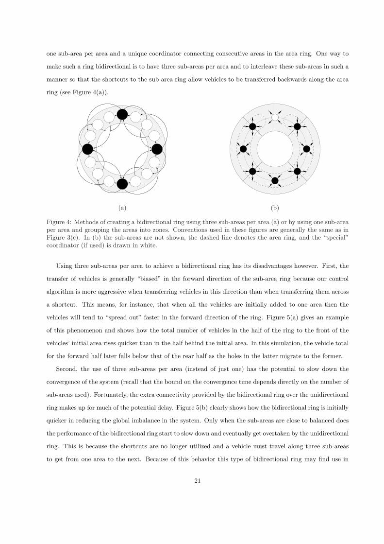
one sub-area per area and a unique coordinator connecting consecutive areas in the area ring. One way to

make such a ring bidirectional is to have three sub-areas per area and to interleave these sub-areas in such a

manner so that the shortcuts to the sub-area ring allow vehicles to be transferred backwards along the area

ring (see Figure 4(a)).

(a) (b)

Figure 4: Methods of creating a bidirectional ring using three sub-areas per area (a) or by using one sub-areaper area and grouping the areas into zones. Conventions used in these figures are generally the same as inFigure 3(c). In (b) the sub-areas are not shown, the dashed line denotes the area ring, and the “special”coordinator (if used) is drawn in white.

Using three sub-areas per area to achieve a bidirectional ring has its disadvantages however. First, the

transfer of vehicles is generally “biased” in the forward direction of the sub-area ring because our control

algorithm is more aggressive when transferring vehicles in this direction than when transferring them across

a shortcut. This means, for instance, that when all the vehicles are initially added to one area then the

vehicles will tend to “spread out” faster in the forward direction of the ring. Figure 5(a) gives an example

of this phenomenon and shows how the total number of vehicles in the half of the ring to the front of the

vehicles’ initial area rises quicker than in the half behind the initial area. In this simulation, the vehicle total

for the forward half later falls below that of the rear half as the holes in the latter migrate to the former.

Second, the use of three sub-areas per area (instead of just one) has the potential to slow down the

convergence of the system (recall that the bound on the convergence time depends directly on the number of

sub-areas used). Fortunately, the extra connectivity provided by the bidirectional ring over the unidirectional

ring makes up for much of the potential delay. Figure 5(b) clearly shows how the bidirectional ring is initially

quicker in reducing the global imbalance in the system. Only when the sub-areas are close to balanced does

the performance of the bidirectional ring start to slow down and eventually get overtaken by the unidirectional

ring. This is because the shortcuts are no longer utilized and a vehicle must travel along three sub-areas

to get from one area to the next. Because of this behavior this type of bidirectional ring may find use in

21

situations where it is more important to reduce large imbalances quickly than to achieve the fastest possible

convergence to a globally balanced state.

Another method of creating a bidirectional ring is shown in Figure 4(b). This method uses only one

sub-area per area and the interconnection consists of an area ring which is first “flattened” into a line and

pairs of areas merged into zones (i.e., areas 1 and NA physically overlap to create a zone, as do areas 2 and

NA − 1, etc.). The line of zones is then made into a ring by connecting its two ends. The result is a ring

of zones in which vehicles can flow in either direction. Without any additional modification this system will

converge to a state where the global zone imbalance is at most two (since any two areas will differ by no more

than one) and by using the line modification discussed in [1] (i.e., having a “special” coordinator use the

control algorithm rules from part 3(a) for s? = s+1 instead of those from part 3(b)) the system will converge

to a single equilibrium point in which the zones are globally balanced. Although this bidirectional ring setup

out performs both the previous setup and the unidirectional ring (Figure 5(b)) and exhibits less biasing

(not shown), it has a few disadvantages. First, achieving globally balanced zones comes from stopping the

circulation of the excess vehicles in the balanced areas, which is undesirable in situations with a low vehicle

to area ratio. Second, in certain circumstances this modification also has the potential to slow down system

convergence (note how it takes much longer for this interconnection to go from a global imbalance of two

to zero when compared to the other rings). Third, if the ring is only part of a larger interconnection, then

the use of two areas to cover the same physical region may hurt the overall performance of the system. Of

course this last remark applies to the first bidirectional ring setup as well because it uses three sub-area to

cover an area.

0 10 20 30 40 50 60 700

5

10

15

20

25

30

time (one unit=length of maximum delay)

vehi

cle

tota

ls

area 1−5areas 7−11

0 10 20 30 40 50 600

10

20

30

40

50

time (one unit=length of maximum delay)

glob

al im

bala

nce

unidirectional ringbidirectional ring (3 sub−areas per area)bidirectional ring (2 areas per zone)

(a) (b)

Figure 5: Performance of bidirectional rings. Plot (a) gives the time history of the number of vehicles ineach half of an eleven area bidirectional ring (of the type shown in Figure 4(a)) when 55 vehicles are initiallyplaced in area six. Plot (b) gives the time history of the global imbalance in the various rings (10 areas each)when all the vehicles (100) are initially placed in one area.

22

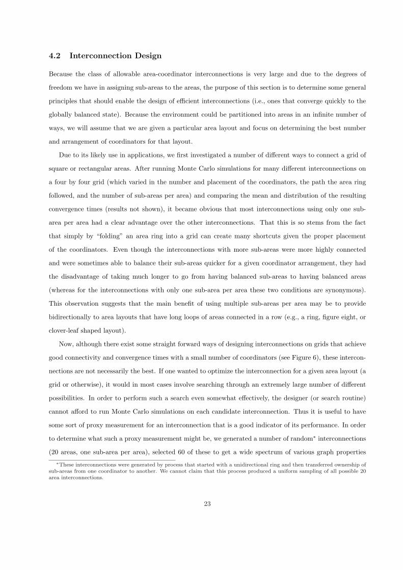
4.2 Interconnection Design

Because the class of allowable area-coordinator interconnections is very large and due to the degrees of

freedom we have in assigning sub-areas to the areas, the purpose of this section is to determine some general

principles that should enable the design of efficient interconnections (i.e., ones that converge quickly to the

globally balanced state). Because the environment could be partitioned into areas in an infinite number of

ways, we will assume that we are given a particular area layout and focus on determining the best number

and arrangement of coordinators for that layout.

Due to its likely use in applications, we first investigated a number of different ways to connect a grid of

square or rectangular areas. After running Monte Carlo simulations for many different interconnections on

a four by four grid (which varied in the number and placement of the coordinators, the path the area ring

followed, and the number of sub-areas per area) and comparing the mean and distribution of the resulting

convergence times (results not shown), it became obvious that most interconnections using only one sub-

area per area had a clear advantage over the other interconnections. That this is so stems from the fact

that simply by “folding” an area ring into a grid can create many shortcuts given the proper placement

of the coordinators. Even though the interconnections with more sub-areas were more highly connected

and were sometimes able to balance their sub-areas quicker for a given coordinator arrangement, they had

the disadvantage of taking much longer to go from having balanced sub-areas to having balanced areas

(whereas for the interconnections with only one sub-area per area these two conditions are synonymous).

This observation suggests that the main benefit of using multiple sub-areas per area may be to provide

bidirectionally to area layouts that have long loops of areas connected in a row (e.g., a ring, figure eight, or

clover-leaf shaped layout).

Now, although there exist some straight forward ways of designing interconnections on grids that achieve

good connectivity and convergence times with a small number of coordinators (see Figure 6), these intercon-

nections are not necessarily the best. If one wanted to optimize the interconnection for a given area layout (a

grid or otherwise), it would in most cases involve searching through an extremely large number of different

possibilities. In order to perform such a search even somewhat effectively, the designer (or search routine)

cannot afford to run Monte Carlo simulations on each candidate interconnection. Thus it is useful to have

some sort of proxy measurement for an interconnection that is a good indicator of its performance. In order

to determine what such a proxy measurement might be, we generated a number of random∗ interconnections

(20 areas, one sub-area per area), selected 60 of these to get a wide spectrum of various graph properties

∗These interconnections were generated by process that started with a unidirectional ring and then transferred ownership ofsub-areas from one coordinator to another. We cannot claim that this process produced a uniform sampling of all possible 20area interconnections.

23

and then added the interconnections at either extreme (i.e., the unidirectional ring and the interconnection

with just one coordinator). As shown in the scatter plot of Figure 7(a), it appears as if the average distance

between areas in the interconnection (where the distance between two areas is the minimum number of

inter-area transfers a vehicle would have to make to get from one to the other) has a direct relationship

to its mean convergence time when the number of vehicles is fixed. Although the spread of data points in

the middle of Figure 7(a) makes it hard to determine if those points fit a line or a curve, it appears that

the increase in convergence time with respect to the increase in mean distance is greater for small mean

distances than for large ones. To explore this further we generated seven different 64 area interconnections

by repeatedly giving a single coordinator ring responsibility for more areas (where the specific areas added

at each stage where selected to reduce the diameter and mean distance of the interconnection by as much

as possible). Figure 7(b) clearly shows a logarithmic-like curve connecting the mean convergence times of

these interconnections.

(a) (b) (c)

Figure 6: A fairly efficient method for interconnecting a grid of areas (similar conventions to those inFigure 4(b)). Layout (a) shows the basic form connected by (black) coordinators, while (b) shows how thebasic form is “folded” into a four by four grid and connected at the ends by an additional (white) coordinator.Layout (c) shows one possibility for a six by six grid.

4.3 Response to a Persistent Disturbance

The results of Section 3 show that when our system is subjected to a one-time disturbance (i.e., the addition

or removal of vehicles) it will return to a balanced state within a finite period of time. Our analytical

results, however, do not show how the system will respond to a persistent disturbance in which vehicles are

continually added to and/or removed from the system. In order to explore the system’s behavior in such

a situation we ran simulations for a line topology in which vehicles were removed from the system at one

end and could be added to it at the other in order to try and maintain a certain vehicle level in the areas.

24

1 2 3 4 5 6 7 8 9 100

500

1000

1500

2000

mean distance between areas in interconnection

mea

n co

nver

genc

e tim

e fo

r in

terc

onne

ctio

n

0 5 10 15 20 25 300

20

40

60

80

100

120

140

160

mean distance between areas in interconnection

conv

erge

nce

time

medianmean

(a) (b)

Figure 7: Plot (a) gives mean distance between areas versus mean convergence time for 62 different 20 areainterconnections using 80 vehicles (120 simulations per interconnection). Plot(b) shows the same relationshipfor seven specific 64 area interconnections (128 simulations per interconnection) plus box plots to illustratethe distribution of convergence times.

(The line topology is a flattened ring with two overlapping areas merged into a zone similar to the setup in

Figure 4(b) but without the special coordinator that reconnects the line into a ring.) This simulation differed

from the others in that we did not simulate the check-in of individual vehicles, but rather simulated the basic

model in Section 2.4 (in order to allow simulations with a large number of vehicles to run in a reasonable

time period). For this simulation there was between 0.9 and 1 time units between events of type eαs→s?

for each sub-area s ∈ S (uniform distribution) and α for these events was the always the maximum value

allowed by the control algorithm. Information updates about the transfer of vehicles was received by other

coordinators between 0.9 and 1 units after the transfer (uniform distribution). Vehicles were removed from

the last zone in the line according to a Poisson process (i.e., vehicles were removed one at a time with the

probability density function of the time between removals τ given by the exponential function λ exp(−λτ)

where λ is the average number of vehicles removed per time unit). Vehicles could be added to (or removed

from) other end of the line once every 0.9 to 1 time units in whatever quantity was necessary to bring the

first zone up to the desired vehicle level.

In order to assess the performance of the system for a given number of zones and value of λ, we first

let the simulation run for 103 time units to allow the system to settle, and then collected data on the time

distribution of the global imbalance for the next 104 time units. For comparison, we also ran the simulation

for the same topology using the local balancing rules used in traditional load balancing (i.e., letting the

destination sub-area be in any area a coordinator was connected to but with all α values determined by

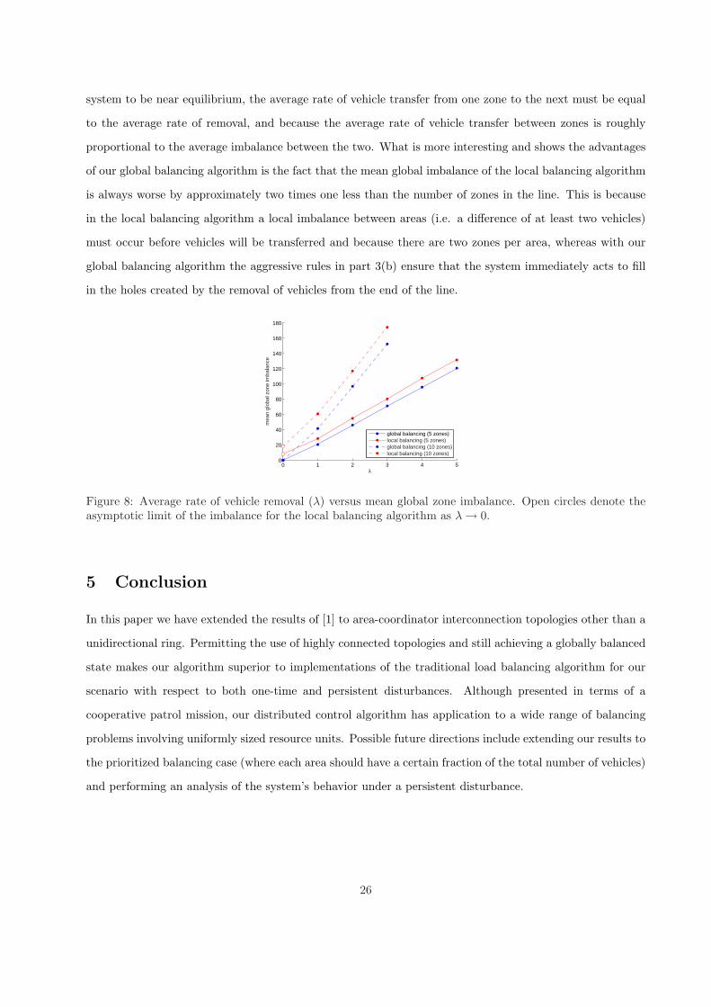
the less aggressive rules in part 3(a) of the control algorithm). As shown in Figure 8 the mean global zone

imbalance varied linearly with the average rate of vehicle removal λ. That this is so is because for the

25

system to be near equilibrium, the average rate of vehicle transfer from one zone to the next must be equal

to the average rate of removal, and because the average rate of vehicle transfer between zones is roughly

proportional to the average imbalance between the two. What is more interesting and shows the advantages

of our global balancing algorithm is the fact that the mean global imbalance of the local balancing algorithm

is always worse by approximately two times one less than the number of zones in the line. This is because

in the local balancing algorithm a local imbalance between areas (i.e. a difference of at least two vehicles)

must occur before vehicles will be transferred and because there are two zones per area, whereas with our

global balancing algorithm the aggressive rules in part 3(b) ensure that the system immediately acts to fill

in the holes created by the removal of vehicles from the end of the line.

0 1 2 3 4 50

20

40

60

80

100

120

140

160

180

λ

mea

n gl

obal

zon

e im

bala

nce

global balancing (5 zones)local balancing (5 zones)global balancing (10 zones)local balancing (10 zones)

Figure 8: Average rate of vehicle removal (λ) versus mean global zone imbalance. Open circles denote theasymptotic limit of the imbalance for the local balancing algorithm as λ → 0.

5 Conclusion

In this paper we have extended the results of [1] to area-coordinator interconnection topologies other than a

unidirectional ring. Permitting the use of highly connected topologies and still achieving a globally balanced

state makes our algorithm superior to implementations of the traditional load balancing algorithm for our

scenario with respect to both one-time and persistent disturbances. Although presented in terms of a

cooperative patrol mission, our distributed control algorithm has application to a wide range of balancing

problems involving uniformly sized resource units. Possible future directions include extending our results to

the prioritized balancing case (where each area should have a certain fraction of the total number of vehicles)

and performing an analysis of the system’s behavior under a persistent disturbance.

26

A Appendix

A.1 Basic Properties

We start by stating a number of simple properties that hold for all k ∈ N and that will be of general use.

Proofs are omitted due to simplicity.

Property 1 : A coordinator c ∈ C’s estimate of the imbalance between the number of vehicles in a sub-area

s ∈ S(c) and the number in a sub-area s? ∈ D(c) is always less than the real imbalance, i.e.,

xcs(k)− xc

s?(k) ≤ xs(k)− xs?(k)

Property 2 : A coordinator c ∈ C will never transfer vehicles from a sub-area s ∈ S(c) to a sub-area

s? ∈ D(c) if xs(k) ≤ xs?(k).

Property 3 : A coordinator c ∈ C will not transfer vehicles out of a sub-area s ∈ S(c) so long as xs(k) =

n(k), nor will it transfer any vehicles to a sub-area s? ∈ D(c) so long as xs?(k) = n(k)

Property 4 : For coordinator c ∈ C and any s ∈ D(c) we have

n(k) ≤ xs(k) ≤ xcs(k)

Property 5 : When xs(k) = n(k) + 1, then coordinator C(s) can only transfer vehicles from sub-area s

“forward” along the ring of sub-areas (i.e., to sub-area s + 1). In addition, it is limited to transferring no

more than one vehicle from sub-area s to sub-area s + 1 per time step (and only if xs+1(k) = n(k)).

A.2 Proof of Lemma 2

Let us focus first on n(k) and show that n(k + 1) ≥ n(k) for all k ∈ N. Take any k ∈ N and any s ∈ S

and consider the number of vehicles in sub-area s at time k + 1. According to the statement of our update

function, xs(k + 1) is equal to xs(k) minus the number of its vehicles transferred by coordinator c = C(s)

(to some sub-area s? ∈ D(c)) and plus the number of vehicles transferred to s by coordinator c′ = C(s− 1)

(from some sub-area s′ ∈ S(c′)). Letting the number of vehicles removed and added to sub-area s at time

step k be denoted by α−s (k) and α+s (k) respectively, the previous statement is equivalent to

xs(k + 1) = xs(k) + α+s (k)− α−s (k) (28)

27

Since α+s (k) and α−s (k) are non-negative, we can bound xs(k + 1) from below as

xs(k + 1) ≥ xs(k)− α−s (k) (29)

We proceed by noting that in all cases of the control algorithm the value of α in an event eαs→s? can be

bounded from above by⌈

xcs(k)− xc

s?(k)2

⌉. Then,

xs(k + 1) ≥ xs(k)−⌈

xcs(k)− xc

s?(k)2

⌉(30)

Using the inequality dqe < q + 1, (30) becomes

xs(k + 1) > xs(k)−(

xcs(k)− xc

s?(k)2

+ 1)

(31)

By employing Property 1 and the fact that both xs(k) and xs?(k) can be no less than n(k) we can proceed

as follows

xs(k + 1) > xs(k)−(

xcs(k)− xc

s?(k)2

+ 1)

≥ xs(k)−(

xs(k)− xs?(k)2

+ 1)

(32)

=12

(xs(k) + xs?(k)

)− 1 (33)

≥ 12

(n(k) + n(k)

)− 1 = n(k)− 1 (34)

But since xs(k + 1) takes on only integer values, xs(k + 1) > n(k)− 1 implies that xs(k + 1) ≥ n(k). Since

this holds for all s ∈ S and all k ∈ N, n(k) must be non-decreasing. A parallel argument shows that n(k) is

non-increasing and is omitted for brevity. ¤

A.3 Proof of Lemma 3

Take any k ∈ N such that n(k) = n(k + 1) = n. In order to prove this lemma, we start by showing that a

sub-area s ∈ S with xs(k) ≥ n+1 cannot become a hole due to its coordinator c = C(s) transferring vehicles

to a sub-area s? ∈ D(c)− {s + 1} (i.e., by a transfer of vehicles across one of the shortcuts to the sub-area

ring). We can start with (29) from the proof of Lemma 2 and use rule (5) from part 3(a) of the control

28

algorithm (since s? 6= s + 1) in conjunction with the inequality bqc ≤ q to proceed in a familiar fashion,

xs(k + 1) ≥ xs(k)− α−s (k)

≥ xs(k)−⌊

xcs(k)− xc

s?(k)2

⌋(35)

≥ xs(k)− xcs(k)− xc

s?(k)2

(36)

≥ xs(k)− xs(k)− xs?(k)2

(37)

=12

(xs(k) + xs?(k)

)(38)

≥ 12

((n + 1) + n

)= n +

12

(39)

But xs(k + 1) ≥ n + 12 implies that xs(k + 1) ≥ n + 1, and thus sub-area s cannot become a hole in this

manner.

It is the case, however, that sub-area s can become a hole when coordinator c transfers vehicles from s

to s + 1. In this case we are interested in the relationship between the values of xs(k), xs(k + 1), xs+1(k),

and xs+1(k + 1). We start by recalling the inequality (33) from the proof of Lemma 2 which gave us a lower

bound on xs(k + 1) based on the most aggressive type of transfer (i.e., one from s to s + 1). Substituting

s? = s + 1,

xs(k + 1) >12

(xs(k) + xs+1(k)

)− 1 (40)

and rearranging to see what values of xs+1(k) can result in xs(k + 1) = n given that xs(k) ≥ n + 1

xs+1(k) < 2xs(k + 1)− xs(k) + 2 (41)

≤ 2n− (n + 1) + 2 (42)

= n + 1 (43)

and of course xs+1(k) < n + 1 implies that xs+1(k) = n. Thus sub-area s can only become a hole at time

k + 1 if sub-area s + 1 is a hole at time k, but since this only happens when coordinator c transfers vehicles

into sub-area s+1 and no vehicles will be transferred out of s+1 (Property 3), then it must be the case that

xs+1(k + 1) ≥ n + 1. Thus the creation of a new hole at sub-area s must be accompanied by the elimination

of a hole at sub-area s + 1. ¤

29

A.4 Proof of Lemma 4

Take any k ∈ N such that n(k) = n(k + 1) = n and any sub-area s such that xs(k) ≥ n + 2. If coordinator

c = C(s) does not transfer any vehicles out of s at time k, then clearly (21) holds. Let us examine what

happens when coordinator c does transfer vehicles from s to some destination s? by considering the cases

s? = s + 1 and s? 6= s + 1 separately.

Case 1: s? ∈ D(c)−{s + 1}. The inequality (38) in Lemma 3 is a lower bound on xs(k + 1) for a vehicle

transfer of this type, so we can simply proceed from there using xs(k) ≥ n + 2,

xs(k + 1) ≥ 12

(xs(k) + xs?(k))

≥ 12xs?(k) +

12n + 1 (44)

Let us evaluate (44) in two sub-cases that depend on the value of xs?(k).

Case 1a: xs?(k) ≥ n + 1. In this case s? is not a hole, and (44) gives us xs(k + 1) ≥ n + 32 which implies

that xs(k + 1) ≥ n + 2 and so sub-area s would remain a hill, thus satisfying condition (21).

Case 1b: xs?(k) = n. Here (44) tells us that xs(k + 1) ≥ n + 1 and thus the hill at sub-area s may

disappear but the hole at sub-area s? gets eliminated, thus satisfying condition (23). (One might worry

about the hole at s? moving to s? − 1 at the same time step and thereby avoiding elimination, but recall

that since s? ∈ D(c), we have s?− 1 ∈ S(c). Thus for this to happen, coordinator c would have to make two

simultaneous transfers of vehicles and this is explicitly prohibited by part 1 of the control algorithm.)

Case 2: s? = s + 1. For this case we can use (40) from Lemma 3 to get a lower bound on xs(k + 1) after

a transfer of vehicles from s to s + 1 when we have xs(k) ≥ n + 2,

xs(k + 1) >12

(xs(k) + xs+1(k)

)− 1

≥ 12xs+1(k) +

12n (45)

And we can evaluate (45) depending on the value of xs+1(k) using three sub-cases.

Case 2a: xs+1(k) ≥ n + 2. Here (45) gives us xs(k + 1) > n + 1 (implying xs(k + 1) ≥ n + 2) and thus

sub-area s would remain a hill and condition (21) is satisfied.

Case 2b: xs+1(k) = n. In this case (45) tells us that xs(k + 1) > n (implying xs(k + 1) ≥ n + 1) so as in

Case 1b it may be that the hill at s disappears but only because a hole at s + 1 gets eliminated (so either

condition (21) or condition (23) is satisfied).

Case 2c: xs+1(k) = n + 1. This sub-case is somewhat more complicated as it depends on the actions of

30

coordinator C(s + 1). Inequality (45) gives us that xs(k + 1) > n + 12 (implying xs(k + 1) ≥ n + 1) so the

hill at sub-area s may disappear. Now, since xs+1(k) = n + 1, Property 5 tells us that coordinator C(s + 1)

is limited to transferring at most one vehicle from s + 1 to s + 2. If it does not transfer a vehicle at time k,

then xs(k + 1) ≥ n + 2 due to coordinator c’s transfer of vehicles from s to s + 1, and so a hill is created

at sub-area s + 1, thus satisfying condition (22). On the other hand, if coordinator C(s + 1) does transfer a

vehicle from s + 1 to s + 2 at time k it must be because s + 2 is a hole (Property 2), but since coordinator

c is transferring at least one vehicle from s to s + 1, sub-area s + 1 will experience no net loss and we have

xs+1(k + 1) ≥ xs+1(k) = n + 1. Thus if the hill at s does disappear without creating a hill at s + 1, it is

because a hole at s + 2 was eliminated, thus satisfying condition (23).

The case analysis above has covered all possibilities and has shown that at least one of the three conditions

of Lemma 4 always holds. ¤

A.5 Proof of Theorem 1

The essence of Lemmas 3 and 4 was to define the possible behavior of the holes and hills, i.e., to establish

that holes may move backwards on the sub-area ring (or be eliminated) while the hills may move forward on

the sub-area ring (and can only be eliminated when a hole is eliminated at the same time). In what follows,

we will show that holes and hills must move in this manner and that this movement ensures the elimination

of at least one hole within a bounded length of time.

Take any k ∈ N such that x(k) ∈ X − XA, and assume that n(k′) is equal to some constant n for all

k′ ≥ k (otherwise (24) holds trivially). It is always the case that there exists at least one sub-area which

is a hole, and since x(k) 6∈ XA it must also be the case that there is at least one sub-area that is a hill

(if not then xs(k) ∈ {n(k), n(k) + 1} which implies x(k) ∈ XA). Furthermore, whenever there are both

holes and hills there must exist either at least one hole s and one hill s such that the block of sub-areas

s + 1, s + 2, . . . , s − 2, s − 1 is a plateau, or at least one hole and hill such that s + 1 = s. For now, let us

assume that there is no hill/hole pair (s, s) such that s+1 = s at time step k and let us show that the system

must evolve to the point where there is at least one such pair. Let s and s be the hill and hole guaranteed

to exist with a connecting plateau s + 1, s + 2, . . . , s − 2, s − 1 at time step k. Since s + 1 6= s this plateau

must contain at least one sub-area. We now determine what happens depending on the locations of s and s

in the sub-area ring. Specifically, we will show that one of the sub-areas of the plateau will become either a

hole or a hill within a finite number of time steps or else a hole is eliminated.

Case 1: s− 1 6= rA(s−1). In this case the leading edge of the plateau is not the last sub-area in its area.

This is the easiest case to analyze because it implies that coordinator C(s − 1) does not have the extra

31

responsibility for balancing area A(s − 1) and thus part 3(c) of the control algorithm does not come into

play. Now, if at any time step k′ ≥ k one or more vehicles are added to a sub-area s′ in the plateau besides

s− 1, then s′ becomes a hill at k′ + 1 (because Property 5 ensures that no vehicles will be moved out of any

of these sub-areas at time time k′). If one or more vehicles is transferred to sub-area s − 1 at time k′ ≥ k

then either either s−1 becomes a hill and/or the hole at sub-area s moves to sub-area s−1 at the same time

and is eliminated. Since both these situations result in one of our desired outcomes, we need only proceed

with our argument for the case in which no vehicles are added to any of the plateau sub-areas from time

step k on.

Now according to Lemma 3, only one of three things may happen to the hole at s at each time step, 1) it

remains a hole, 2) it moves to sub-area s− 1, or 3) it gets eliminated (without the generation of a new hole

at s−1). Disregarding the third possibility (because it automatically gives us a desired result), it is our task

to show that the second possibility eventually happens (i.e., that coordinator c = C(s − 1) will eventually

transfer a vehicle from s− 1 to s). Now, if coordinator c has not made such a transfer by time step k + B,

then according to (11) and (13) from the description of the allowed trajectories EA we will have

n = xs(k′) ≤ xcs(k

′) ≤ xs(k) = n for all k′ ≥ k + B (46)

And (under our assumption about no vehicles being added to the plateau sub-areas) we also have that

xs−1(k′) = n + 1 for all k′ ≥ k and so by (10) and (12) we will have

n + 1 = xs−1(k) ≤ xcs−1(k

′) ≤ xs−1(k′) = n + 1 for all k′ ≥ k + B (47)

Therefore, for all k′ ≥ k+B coordinator c’s estimate of the imbalance between s−1 and s, xcs−1(k

′)− xcs(k′),

is accurate and equal to one. Thus when c attempts to balance sub-area s− 1 (which it must do within the

next B time steps according to the definition of EA), Property 5 reminds us that it can only transfer one

vehicle to s and part 3(b) of the control algorithm tells us that it will indeed do this. Thus by time step

k + 2B, the hole at s moves to s− 1 (or one of our previous assumptions was violated at some time step k′

between k and k + 2B and either a sub-area in the plateau became a hill or the hole at s was eliminated).

Case 2: s 6= rA(s). In this case, the hill is not located in the last sub-area for its area. This case contains

some of the most complex logic of our analysis and we will use some of its results again in Case 3b below.

This time we start by assuming that after time step k the hole at s does not move to s − 1 and that no

vehicles are added to any plateau sub-area either (if either of these things happen, then we have the desired

result automatically). Under those assumptions, we show that coordinator c = C(s) will eventually transfer

32

at least one vehicle from s to s + 1. Now, Property 2 ensures that no vehicles will be removed from sub-area

s + 1 as long as the hole stays at sub-area s. Since no vehicles are added to any plateau sub-area after time

k, the The inequalities (11) and (13) give us

n + 1 = xs+1(k′) ≤ xcs+1(k

′) ≤ xs+1(k′) = n + 1 for all k′ ≥ k + B (48)

So coordinator c has an accurate estimate of xs+1(k′) for all k′ ≥ k + B. Now, in order to show that

coordinator c will eventually transfer a vehicle from s to s + 1, we first need to show that xcs(k

′) ≥ n + 2 for

all k′ greater than some value. If coordinator c does not transfer any vehicles out of sub-area s from time

step k on, then we can use (12) in order to show that

xcs(k

′) ≥ xs(k) ≥ n + 2 for all k′ ≥ k + B (49)

Unfortunately, coordinator c is not generally restricted from removing vehicles from sub-area s and the logic

leading up to (49) does not hold when coordinator c makes such a removal. We can, however, get an identical

bound using another line of reasoning. Let k? ≥ k be some time step such that eαs→s? ∈ e(k?) for some

s? ∈ D(c) and some α ≥ 1 (i.e., a time step when coordinator c transfers vehicles out of sub-area s). If

s? = s + 1, then we have our desired result. If s? 6= s + 1 then we can analyze the value of xcs(k

? + 1). We

start with the following equation which describes the update of coordinator c’s estimate for xs

xcs(k

? + 1) = xcs(k

?)− α−s (k?) + βcs(k

?) (50)

where α−s (k?) is the number of vehicles c transferred out of sub-area s at time step k? and βcs(k

?) is the

number of previously unseen vehicles that check in with coordinator c at time step k?. We know βcs(k

?) is

non-negative and since s? 6= s + 1 rule (5) from part 3(a) of the control algorithm determines the upper

bound on α−s (k?). We can thus proceed as follows,

xcs(k

? + 1) ≥ xcs(k

?)− α−s (k?) (51)

≥ xcs(k

?)−⌊

xcs(k

?)− xcs?(k?)

2

⌋(52)

≥ xcs(k

?)− xcs(k

?)− xcs?(k?)

2(53)

=12

(xc

s(k?) + xc

s?(k?))

(54)

If sub-area s? is a hole at time k?, then this transfer eliminates a hole and we have a desired result (recall

33

that if s? was a hole, then it could not escape elimination by moving to s? − 1 at k? because C(s? − 1) = c

and coordinator c is limited to transferring vehicles from at most one one sub-area in S(c) per time step).

Proceeding in the case where s? is not a hole, we have xs?(k?) ≥ n+1 and thus (11) gives us that xcs?(k?) ≥

n + 1 as well. In addition, since α−s (k?) ≥ 1 it must be the case that the condition of rule (5) is met at time

step k?, so we also have xcs(k

?) ≥ xcs?(k?) + 2. We can use these two inequalities to evaluate (54) as follows,

xcs(k

? + 1) ≥ 12

(xc

s(k?) + xc

s?(k?))

≥ 12

((xc

s?(k?) + 2) + xcs?(k?)

)(55)

= xcs?(k?) + 1 (56)

≥ n + 2 (57)

The implication of (57) is that if coordinator c transfers some vehicles to a sub-area s? 6= s + 1 at time step

k? ≥ k, then for all k′ ≥ k? + 1 coordinator c’s estimate for sub-area s satisfies xs(k′) ≥ n + 2. This is

because events e+βc,s after time step k? cannot decrease xc

s and another event eαs→s? just gives us (57) again.

In summary, coordinator c must try and balance sub-area s at some time k′ such that k + B ≤ k′ ≤k + 2B − 1 and when it does it is either the case that it has not transferred any vehicles out of s from k to

k′ − 1 (in which case (49) applies) or that it transferred vehicles out of s at least once in that interval (in

which case (57) applies). Since both (49) and (57) give us xcs(k

′) ≥ n + 2, and we have already shown that

xcs+1(k

′) = n+1 for the values of k′ under consideration, we have that c must transfer at least one vehicle from

s to s + 1 (given rule (7) in part 3(b) of the control algorithm) provided that xcs+1(k

′) = mins′∈D(c) xcs′(k

′)

(see part 2 of the control algorithm). Fortunately, it can only be the case that xcs+1(k

′) is not such a minimum

when there is a sub-area s? ∈ D(c) such that xcs?(k′) = n, but Property 4 showed us that that would imply

xs?(k′) = n, and so when coordinator c transferred vehicles to this sub-area (instead of sub-area s + 1) then

it would eliminate a hole (which is also a desired result). Thus the hill at s moves to s + 1 by time step

k + 2B (and/or another sub-area in the plateau became a hill and/or the hole at s moved to s − 1 and/or

some hole was eliminated at an earlier time step).

Case 3: s − 1 = rA(s−1) and s = rA(s). In this case both s − 1 and s are the last sub-areas in their

respective areas (which is the only possibility not already covered by either Case 1 or Case 2). Because of

the location of s − 1 and s, analysis of this case involves looking at the function h defined by (9) in part

3(c) of the control algorithm. For the sake of generality, we show here that each coordinator Ra may use a

34

different function ha in lieu of h so long as one of the following properties holds for all a ∈ A.

xRa

s′ (k) > xRas+1(k) for all s′ ∈ S(a) ⇒ ha(xRa(k)) = 1 (58)

xRa

s′ (k) < xRas (k) for all s′ ∈ S(a + 1) ⇒ ha(xRa(k)) = 1 (59)

To clarify, the functions ha, a ∈ A, must all satisfy the same property. That is to say that if ha satisfies

property (58) but not property (59), then ha′ must satisfy property (58) as well for every a′ ∈ A. Our

purpose here is to leave open the possibilities of using functions ha 6= h and having setups with a differing

number of sub-areas per area (i.e., we show the most general conditions for ha under which the system is

guaranteed to balance the sub-areas). We now continue with our case analysis based on which property the

functions ha, a ∈ A satisfy.

Case 3a: ha satisfies (58) for all a ∈ A. In this case we will be able to show coordinator c = C(s− 1) fills

in the hole at sub-area s within 2B time steps. Since both s and s − 1 are the last sub-areas in their area,

it follows that s 6∈ A(s − 1) and thus every sub-area in area A(s − 1) must be part of the plateau. Let us

proceed directly to consideration of the case in which no vehicles are added to the plateau and the hole at

s is not eliminated after time step k (because this leads automatically to a desired result). As in Case 1, if

coordinator c does not transfer a vehicle from s − 1 to s by time k + B, we will have that xcs(k

′) = n and

xcs−1(k

′) = n + 1 for all k′ ≥ k + B. We also have xs(k′) = n + 1 for all k′ ≥ k for each sub-area s in the

plateau (because no vehicles are added to any of those sub-areas and Property 2 ensures that no vehicles

will be removed as long as the hole stays at s). The inequalities (12) and (13) then give us

n + 1 = xs(k′) ≤ xcs(k

′) ≤ xs(k′) = n + 1 for all k′ ≥ k + B (60)

for all sub-areas s in the plateau and for s ∈ S(A(s − 1)) in particular. Letting a = A(s − 1) and noting

that Ra = c (because ra = s− 1), we have that (60) holds for all s ∈ S(a). This means that condition (58)

from part 3(c) of the control algorithm is met. Coordinator c must then attempt to balance sub-area s− 1

at least once between time step k + B and k + 2B, and when it does the control algorithm will dictate that

it transfer a vehicle from s− 1 to s. Thus the hole must move from s to s− 1 by time step k + 2B (and/or

some sub-area in the plateau became a hill and/or the hole at s was eliminated).

Case 3b: ha satisfies (59) for all a ∈ A. In this case we will be able to show coordinator c = C(s) will

transfer a vehicle to sub-area s + 1 within 2B time steps. Since s and s − 1 are the last sub-areas in their

respective areas, it must be that every sub-area in area A(s + 1) must be part of the plateau. Let us again

proceed directly to consideration of the case in which no vehicles are added to the plateau and the hole at s

35

is not eliminated after time step k (because either result gives us what we want automatically). As shown

in Case 2, it must be the case that xcs(k

′) ≥ n + 2 and xcs+1(k

′) = n + 1 for all k′ ≥ k + B. Since no vehicles

are added to or removed from the plateau after time step k, then (60) again holds for all the sub-areas s

in the plateau, and this time for s ∈ S(A(s) + 1) in particular. Letting a = A(s) and noting that Ra = c

(because ra = s), we have that (60) holds for all s ∈ S(a + 1). This means that condition (59) from part

3(c) of the control algorithm is met. Coordinator c must then attempt to balance sub-area s at least once

between time step k + B and k + 2B, and when it does the control algorithm will dictate that it transfer a

vehicle to s + 1. Thus the hill must move from s to s + 1 by time step k + 2B (and/or some other sub-area

in the plateau became a hill and/or the hole at s was eliminated).

The above case analysis have proven that, in the absence of a hole being eliminated, at least one sub-area

in the plateau between the hill s and the hole s becomes either a hill or a hole by time step k + 2B. With

this information we can see that at time step k + 2B there must be a hill and hole separated by a plateau

that is at least one sub-area shorter than the one we were considering at time step k. Since this process is

guaranteed to keep repeating, we will eventually get to the point where we have a hill s and hole s such that

s+1 = s. Specifically, since a plateau can originally consist of no more than NS − 2 sub-areas (i.e., the total

number of sub-areas minus the sub-areas s and s) we will have this condition no later than k + 2B(NS − 2).

We now show that coordinator c = C(s) will eventually transfer a vehicle from s to s thereby eliminating

the hole at s. In the case analysis above, we have already shown that for k′ ≥ k + 2B(NS − 2) + B that

xcs(k

′) ≥ n+2 and xcs(k′) = n (unless, of course, c transferred a vehicle from s to s or to another sub-area that

is a hole prior to time step k′, in which case the hole is eliminated). Thus let k′ ≤ k + 2B(NS − 2) + 2B − 1

be the first time step after k + 2B(NS − 2) + B when c attempts to balance sub-area s, and note that since

xcs(k′) = n and xc

s′(k′) ≥ xs′(k′) ≥ n, part 2 of the control algorithm states that coordinator c is forced to

transfer vehicles from s to s. Since have xcs(k

′)− xcs(k

′) ≥ 2 rule (7) in part 3(b) of the control algorithm will

apply and thus at least one vehicle is transferred to sub-area s (thereby eliminating the hole). In conclusion,

we have shown that for some T ≤ 2B(NS − 1), either (24) or (25) holds, thus proving the theorem to be

true. ¤

A.6 Proof of Lemma 6

To prove this lemma we verify that each of the three conditions in (9) for which h(xRa(k)) = 1 implies

that ya(k) > ya+1(k). First, since x(k) ∈ XA we can apply (14) from the definition of EA. Thus when

yRaa (k) > yRa

a+1(k) we automatically have ya(k) > ya+1(k).

Second, by definition we can have h(xRa(k)) = 1 only if xRara

(k) = xRara+1(k)+1, and since x(k) ∈ XA ⊂ XA

36

this can only happen when xRara

(k) = xra(k) = n + 1 and xRa

ra+1(k) = xra+1(k) = n (i.e., because of the

definition of XA and the inequalities (10) and (11) we know that xRara

(k) ≤ xra(k) ≤ n + 1 and xRa

ra+1(k) ≥xra+1(k) ≥ n). Now, if xRa

s > xRara+1(k) = n for all s ∈ S(a), then yRa

a (k) ≥ p(n + 1). But since (14) gives

us ya(k) ≥ yRaa (k) and x(k) ∈ XA implies that ya(k) ≤ p(n + 1), we must have that ya(k) = p(n + 1). Since

xra(k) = n and x(k) ∈ XA we also know that ya+1(k) ≤ n + (p− 1)(n + 1) = p(n + 1)− 1 and so again we

have ya(k) > ya+1(k).

Lastly, in a similar argument to the one just above, if xRas (k) < xRa

ra(k) = n+1 for all s ∈ S(a+1), then

we have that yRaa+1(k) ≤ pn and since x(k) ∈ XA it must also be the case that ya+1(k) ≥ pn which implies

ya+1(k) = pn. Now since xra(k) = n + 1 and x(k) ∈ XA we know that ya(k) ≥ (n + 1) + (p− 1)n = pn + 1

and so ya(k) > ya+1(k) once again.

We have proven above that when x(k) ∈ XA then h(xRa(k)) = 1 only if ya(k) > ya+1(k). We stress that

this result does not necessary apply when x(k) 6∈ XA. ¤

A.7 Proof of Lemma 8

Take any k ∈ N such that x(k) ∈ XA and ya(k) > ya+1(k) for some a ∈ A. In order show that there

exists a time k + T when a vehicle is transferred from sub-area ra to ra + 1 (and thus from area a to area

a + 1) we show the system must evolve so that for some k′ < ∞ we will have xRara

(k′) = xRara+1(k

′) + 1,

yRaa (k′) > yRa

a+1(k′), and eα

ra→ra+1 ∈ e(k′) (i.e., there exists a time step k′ where coordinator Ra attempts

to balance sub-area ra and h(xRa(k′)) = 1). Now if coordinator Ra does not transfer a vehicle from ra to

ra + 1 between time step k and time step k + B then because x(k) ∈ XA the inequalities (15) and (16) from

the definition of EA give us

yRaa (k′) ≥ ya(k) > ya+1(k) ≥ yRa

a+1(k′) for all k′ ≥ k + B (61)

and so we only really need to figure out how long it may take to get xRara

(k′) = xRara+1(k

′) + 1, or more

specifically, xRara

(k′) = n + 1 and xRara+1(k

′) = n. Now x(k) ∈ XA and ya(k) > ya+1(k) implies that there is

at least one sub-area s ∈ S(a) such that xs(k) = n + 1. If we let s be the closest such sub-area to ra (i.e.,

so that xs′(k) = n for all s′ ∈ {s + 1, . . . , ra}) then because Lemma 1 showed us that the hole at s + 1 must

move to s within 2B time steps (but only because s + 1 6= ra + 1). Thus it will take at most 2B(p − 1)

time steps to arive at the situation where xra(k′) = n + 1 and at most another B to get xRara

(k′) = n + 1.

Similarly (and simultaneously) it can take at most 2B(p− 1) + B time steps to get xRara+1(k

′) = n. Thus the

necessary conditions for h(xRa) = 1 are acheived by time step k + max{B, 2B(p− 1) + B} and it takes only

37

at most another B time steps for a partial event eαra→ra+1 to occur with α = 1. So, the upper bound on T

is given by max{2B, 2Bp} ≤ 2Bp. ¤

A.8 Proof of Theorem 2

It should be clear from Lemmas 6 and 8 that when x(k) ∈ XA the vehicle balancing system behaves

in essentially the same manner as the system in [1] consisting of a unidirectional ring area-coordinator

interconnection (i.e., vehicles may only be transferred in one direction around the area ring, vehicles will

only be transferred from area a to area a + 1 if the number of vehicles in a is greater than the number

in a + 1, vehicles will eventually be transferred if there is such an imbalance between two areas). Thus to

prove this theorem we need only to adapt the final result of [1]. In that paper the longest period of time it

could take to raise the minimum number of vehicles per area was given by 2B⌈

N

2

⌉(N − 1) where N was

the number of areas (NA here) and 2B was largest number of time steps it could take for a coordinator

to transfer a vehicle from an area with more vehicles to one with less (2Bp here). Now the values of m

can be bounded from above by p(n + 1) − 1 (otherwise L ≥ p(n + 1)NA and we have the contradiction

n =⌊

p(n + 1)NA

NS

⌋=

⌊p(n + 1)NA

pNA

⌋= n+1) and the smallest number of vehicles per area for x(k) ∈ XA is

pn. Thus it could take at most 2Bp

⌈NA

2

⌉(NA − 1)(p− 1) time steps for the state of the system to go from

any state in XA to XB . ¤

References

[1] B. J. Moore and K. M. Passino, “Distributed balancing of AAVs for uniform surveillance coverage

(Full version submitted to International Journal of Robust and Nonlinear Control),” in 44nd IEEE

Conference on Decision and Control, (Seville, Spain), December 2005.

[2] Y. Liu, J. B. Cruz, and A. G. Sparks, “Coordinating networked uninhabited air vehicles for persistent

area denial,” in 43rd IEEE Conference on Decision and Control, (Paradise Island, Bahamas), pp. 3351–

3356, December 2004.

[3] E. Frazzoli and F. Bullo, “Decentralized algorithms for vehicle routing in a stochastic time-varying

environment,” in 43rd IEEE Conference on Decision and Control, (Paradise Island, Bahamas), pp. 3357–

3363, December 2004.

38

[4] J. Cortes, S. Martinez, and F. Bullo, “Coordinated deployment of mobile sensing networks with limited-

range interactions,” in 43rd IEEE Conference on Decision and Control, (Paradise Island, Bahamas),

pp. 1944–1949, December 2004.

[5] D. P. Bertsekas and J. N. Tsitsiklis, Parallel and Distributed Computation: Numerical Methods. Bell-

mont, MA: Athena Scientific, 1997.

[6] K. L. Burgess and K. M. Passino, “Stability analysis of load balancing systems,” International Journal

of Control, vol. 61, pp. 357–393, Feb 1995.

[7] J. Finke, K. M. Passino, and A. Sparks, “Cooperative control via task load balancing for networked

uninhabited autonomous vehicles,” in 42nd IEEE Conference on Decision and Control, (Maui, Hawaii),

pp. 31–36, December 2003.

[8] A. Cortes, A. Ripoll, F. Cedo, M. Senar, and E. Luque, “An asynchronous and iterative load balancing

algorithm for discrete load model,” Journal of Parallel and Distributed Computing, vol. 62, pp. 1729–

1746, December 2002.

[9] R. Els and B. Monien, “Load balancing of unit size tokens and expansion properties of graphs,” in

SPAA ’03: Proceedings of the fifteenth annual ACM symposium on Parallel algorithms and architectures,

pp. 266–273, ACM Press, 2003.

[10] D. Henrich, “The liquid model load balancing method,” Journal of Parallel Algorithms and Applications,

Special Issue on Algorithms for Enhanced Mesh Architectures, vol. 8, pp. 285–307, 1996.

[11] B. J. Moore and K. M. Passino, “Spatial balancing of autonomous vehicle resources,” in Proceedings of

the American Control Conference (to appear), 2006.

[12] K. L. Burgess and K. M. Passino, Stability Analysis of Discrete Event Systems. New York, NY: John

Wiley and Sons, 1998.

39