DISTRIBUTED HYPER-PARAMETER OPTIMIZATION · PDF file• Variation of Gradient Descent: ......

Copyr i g ht © 2016, SAS Ins t i tu t e Inc . A l l r ights reser ve d .

DISTRIBUTED HYPER-PARAMETER

OPTIMIZATION FOR MACHINE LEARNING

YAN XU

DPDA WORKSHOP

SEPT 21, 2016


OUTLINE

1. Background

2. Hyper-parameter Optimization Methods

3. Distributed Computing

4. Experimental Results


BACKGROUND MACHINE LEARNING MODELS

Transformation of relevant data to high-quality descriptive and predictive models

Ex.: Neural Network

• How to determine model configuration?

• How to determine weights, activation

functions?

….

….

….

Input layer Hidden layer Output layer

x1

x2

x3

x4

xn

wij

wjk

f1(x)

f2(x)

fm(x)


BACKGROUND MODEL TRAINING – OPTIMIZATION PROBLEM

• Objective Function

• 𝑓 𝑤 =1

𝑛 𝑖=1𝑛 𝐿 𝑤; 𝑥𝑖 , 𝑦𝑖 + 𝜆1 𝑤 1 +

𝜆2

2𝑤 2

2

• Loss, 𝐿(𝑤; 𝑥𝑖 , 𝑦𝑖), for observation (𝑥𝑖 , 𝑦𝑖) and weights, 𝑤

• Stochastic Gradient Descent (SGD)

• Variation of Gradient Descent: 𝑤𝑘+1 = 𝑤𝑘 − 𝜂𝛻𝑓(𝑤𝑘)

• Approximate 𝛻𝑓 𝑤𝑘 with gradient of mini-batch sample: {𝑥𝑘𝑖 , 𝑦𝑘𝑖 }

• 𝛻𝑓𝑡(𝑤) =1

𝑚 𝑖=1𝑚 𝛻𝐿(𝑤; 𝑥𝑘𝑖 , 𝑦𝑘𝑖)


BACKGROUND MODEL TRAINING – OPTIMIZATION PARAMETERS (SGD)

• Learning rate η

• Too high, diverges

• Too low, slow performance

• Momentum μ

• Too high, could “pass” solution

• Too low, no performance improvement

• Regularization parameters λ1 and λ2

• Too low, has little effect

• Too high, drives iterates to 0

• Other parameters

• Mini-batch size

• Adaptive decay rate

• Annealing rate

• Communication frequency, ……


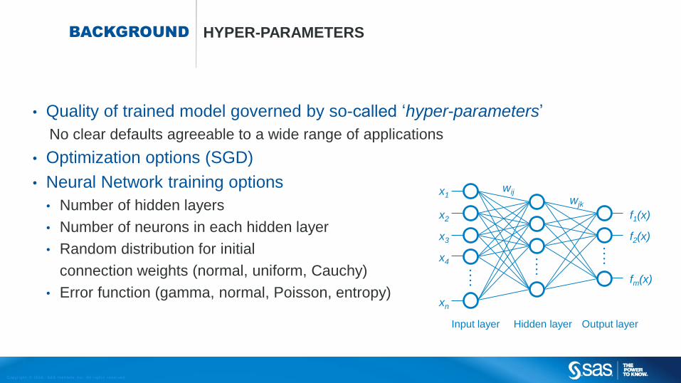
BACKGROUND HYPER-PARAMETERS

• Quality of trained model governed by so-called ‘hyper-parameters’

No clear defaults agreeable to a wide range of applications

• Optimization options (SGD)

• Neural Network training options

• Number of hidden layers

• Number of neurons in each hidden layer

• Random distribution for initial

connection weights (normal, uniform, Cauchy)

• Error function (gamma, normal, Poisson, entropy)

….

….

….

Input layer Hidden layer Output layer

x1

x2

x3

x4

xn

wij

wjk

f1(x)

f2(x)

fm(x)


METHODS HOW TO FIND GOOD HYPER-PARAMETER SETTINGS?

• Traditional Approach: manual tuning

Even with expertise in machine learning algorithms and their parameters, best settings

are directly dependent on the data used in training and scoring

• Hyper-parameter Optimization: Grid vs. Random vs. “Real” Optimization

x1

x2

Standard Grid Search

x1

x2

Random Latin Hypercube

x1

x2

Random Search


METHODS MANY CHALLENGES

Tuning objective, T(x), is validation error score (to avoid increased overfitting effect)

T(x)

x

Objective

blows up

Categorical / Integer

Variables Noisy/Nondeterministi

c

Flat-regions.

Node failure


METHODS OUR APPROACH – LOCAL SEARCH OPTIMIZATION (LSO)

Default hybrid search strategy:

1. Initial Search: Latin Hypercube Sampling (LHS)

2. Global search: Genetic Algorithm (GA)

• Supports integer, categorical variables

• Handles nonsmooth, discontinuous space

3. Local search: Generating Set Search (GSS)

• Similar to Pattern Search

• First-order convergence properties

• Developed for continuous variables

All can be parallelized naturally


DISTRIBUTED

COMPUTINGPARALLEL TRAINING VS. PARALLEL TUNING

Set Tuning Parameter

Values

fold++

fold >

nFolds?

Train

node 1 node 2 node n…

Score

node 1 node 2 node n…

Return Results

Parallel Training

yes no

yes

no

Parallel Tuning

Train

node 2Train

node 1

Train

node n

maxIters?

maxEvals?

maxTime?

Tuning loop

Objective loop

…

Score

node 2Score

node 1

Score

node n…

fold >

nFolds?

maxIters?

maxEvals?

maxTime?Return

Results

fold++

Set Tuning

Parms, node 1

fold++

Set Tuning

Parms, node 2

fold++

Set Tuning

Parms, node n

…

…

yesyesno

no

Hybrid

?


Pa

ralle

l &

Se

ria

l, P

ub

/ S

ub

,

Web S

erv

ices, M

Qs

Source-basedEngines

Microservices

UAA

Query

Gen

Folders

CAS

Mgmt

Data

Source

Mgmt

Analytics

GUIs

etc.…

BI

GUIs

Env

Mgr

Model

Mgmt

Log

Audit

UAAUAA

Data

Mgmt

GUIs

In-Memory Engine

In-Cloud

In-Database

In-Hadoop

In-Stream

Solutions

APIs

Infrastructures

Platforms

SAS®

Viya™

PLATFORM

Analytics

Data ManagementFraud and Security Intelligence

Business VisualizationRisk Management

!

Customer Intelligence

Cloud Analytics Services (CAS)

DISTRIBUTED

COMPUTING


EXPERIMENTAL

RESULTSEXPERIMENT SETTINGS

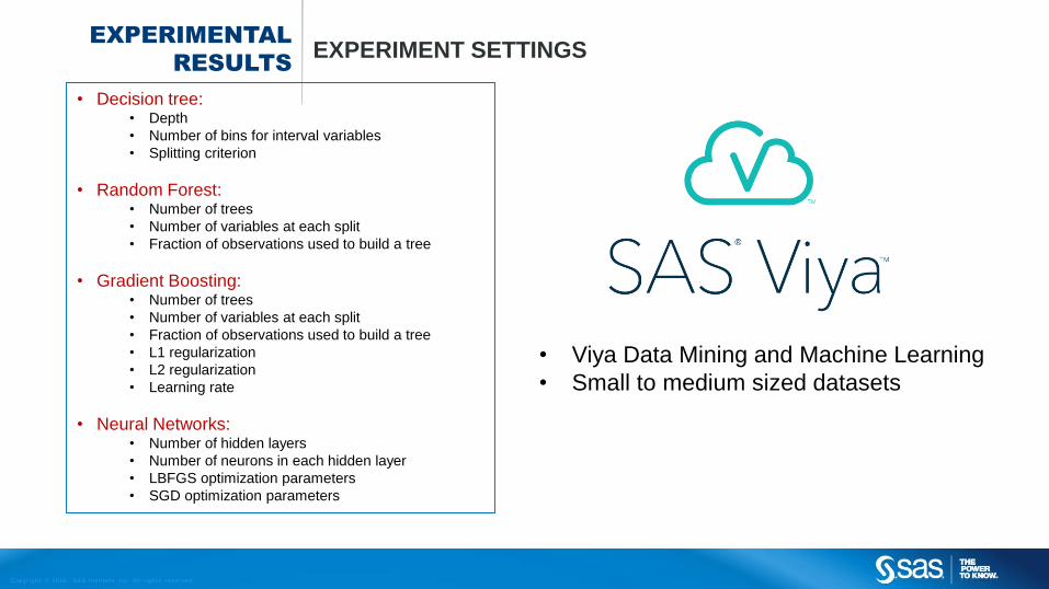
• Decision tree:• Depth

• Number of bins for interval variables

• Splitting criterion

• Random Forest:• Number of trees

• Number of variables at each split

• Fraction of observations used to build a tree

• Gradient Boosting: • Number of trees

• Number of variables at each split

• Fraction of observations used to build a tree

• L1 regularization

• L2 regularization

• Learning rate

• Neural Networks:• Number of hidden layers

• Number of neurons in each hidden layer

• LBFGS optimization parameters

• SGD optimization parameters

• Viya Data Mining and Machine Learning

• Small to medium sized datasets


EXPERIMENTAL

RESULTSEFFECTIVENESS OF THE DIFFERENT TUNING METHODS

• Gradient Boosting

• 6 hyper-parameters

• 15 test problems

• Single 30% validation

partition

• Single machine mode

• Run 10 times each

• LSO (50x5 evaluations)

• LHS (246 samples)

• Random (246 samples)

• Averaged results

Average Error (%)

After Tuning

m s

LSO 10.661 2.193

LHS 11.085 2.324

Random 11.102 2.319

Higher is better

%


EXPERIMENTAL

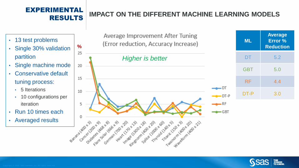
RESULTSIMPACT ON THE DIFFERENT MACHINE LEARNING MODELS



partition

• Single machine mode

• Conservative default

tuning process:

• 5 Iterations

• 10 configurations per

iteration



ML

Average

Error %

Reduction

DT 5.2

GBT 5.0

RF 4.4

DT-P 3.0

Higher is better

%


EXPERIMENTAL

RESULTSMODELS – TIME VS. ACCURACY



partition

• Single Machine mode

• Conservative default

tuning process:

• 5 Iterations

• 10 configurations per

iteration



MLAverage

% Error

Average

Time

(Sec.)

DT 15.3 9.2

DT-P 13.9 12.8

RF 12.7 49.1

GBT 11.7 121.8


EXPERIMENTAL

RESULTSSINGLE PARTITION VS. CROSS VALIDATION

• For each problem:

• Tune with single 30% partition

• Score best model on test set

• Repeat 10 times

• Average difference between

validation error and test error

• Repeat process with 5-fold cross

validation

• Cross validation for small-

medium data sets

• 5x cost increase for sequential

tuning process

• manage in parallel / threaded

environment

under-estimated


EXPERIMENTAL

RESULTSTUNING NEURAL NETWORK MODEL

• Default train, 9.6 % error

• Iteration 1 – Latin Hypercube best,

6.2% error

• Very similar configuration can have very different error

• Best after tuning: 2.6% error

0

20

40

60

80

100

0 50 100 150

Err

or

%

Evaluation

Iteration 1: Latin Hypercube Sample Error

0

2

4

6

8

10

12

0 5 10 15 20

Obje

ctive (

Mis

cla

ssific

ation E

rror

%)

Iteration

Handwritten Data Train 60k/Validate 10k


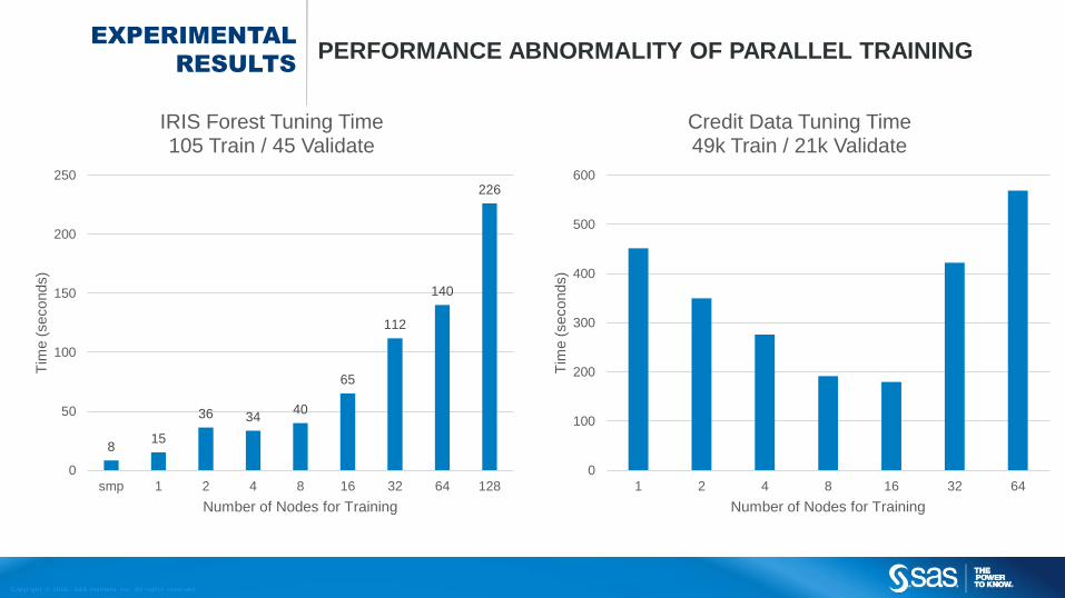
EXPERIMENTAL

RESULTSPERFORMANCE ABNORMALITY OF PARALLEL TRAINING

815

36 3440

65

112

140

226

0

50

100

150

200

250

smp 1 2 4 8 16 32 64 128

Tim

e (

seconds)

Number of Nodes for Training

IRIS Forest Tuning Time105 Train / 45 Validate

0

100

200

300

400

500

600

1 2 4 8 16 32 64

Tim

e (

seconds)

Number of Nodes for Training

Credit Data Tuning Time49k Train / 21k Validate


LSO FOR HYPER-

PARAMETER TUNINGHYBRID – PARALLEL TRAINING AND PARALLEL TUNING

0

2

4

6

8

10

12

2 4 8 16 32

Tim

e (

hours

)

Number of Models Trained in Parallel

Handwritten Data Train 60k / Validate 10k

LHS

GA

GSS

D

NM

…

Train, Score

Node 1

Node 2

Node 3

Node 4

Train, Score

Node 5

Node 6

Node 7

Node 8

Hybrid Solver Manager

..

.

..

.

• Hybrid tuning:

• 4 nodes each training

• n concurrent training


CONCLUSION MANY TUNING OPPORTUNITIES AND CHALLENGES

• Initial Implementation

• SAS® Viya™ Data Mining and Machine Learning

• Other search methods, extending hybrid solver framework

• Bayesian / surrogate-based Optimization

• New hybrid search strategies

• Selecting best machine learning algorithm

• Parallel tuning across algorithms & strategies for effective node usage

• Combining models


THANK YOU!

[email protected]

Date post:	06-Mar-2018
Category:	Documents
Upload:	trankhue
View:	220 times
Download:	0 times

DISTRIBUTED HYPER-PARAMETER OPTIMIZATION · PDF file• Variation of Gradient Descent: ......

Documents