Distributed Intelligent Systems – W10An Introduction to Particle Swarm Optimization and its Application to Benchmark

Functions and Single-Robot Systems

1

Outline• Machine-learning-based methods

– Rationale for embedded systems– Terminology

• Particle Swarm Optimization (PSO)• Comparison between PSO and GA• Application to single-robot systems

– Examples in control design and optimization (obstacle avoidance, homing)

– Examples in system design and optimization (locomotion)

• An introduction to expensive optimization problems and noise resistance

Initialize

Perform main loop

End criterion met?

End

Start

N

Y

2

Rationale and Classification

3

Why Machine-Learning?• Complementary to a model-based/engineering

approaches: when low-level details matter (optimization) and/or good models do not exist (design)!

• When the design/optimization space is too big (infinite)/too computationally expensive (e.g., NP-hard) to be systematically searched

• Automatic design and optimization techniques• Role of the engineer refocused to performance

specification, problem encoding, and customization of algorithmic parameters (and perhaps operators)

4

Why Machine-Learning?

• There are design and optimization techniques robust to noise, nonlinearities, discontinuities

• Possible search spaces: parameters, rules, SW or HW structures/architectures

• Individual real-time adaptation to new or unpredictable environmental/system conditions

5

ML Techniques: Classification Axis 1

– Supervised learning: off-line, a teacher is available

– Unsupervised learning: off-line, teacher not available

– Reinforcement-based (or evaluative) learning: on-line, no pre-established training and evaluation data sets

6

Supervised Learning

– Off-line– Training and test data are separated, a teacher is available– Typical scenario: a set of input-output examples is provided to

the system, performance error given by difference between system output and true/teacher-defined output, error fed to the system using optimization algorithm so that performance is increased over trial

– The generality of the system after training is tested on examples not previously presented to the system (i.e. a “test set” exclusive from the “training set”)

7

Unsupervised Learning

– Off-line– No teacher available, no distinction between training

and test data sets– Goal: structure extraction from the data set – Examples: data clustering, Principal Component

Analysis (PCA) and Independent Component analysis (ICA)

8

Reinforcement-based (or Evaluative) Learning

– On-line– No pre-established training or test data sets– The system judges its performance according to a given metric

(e.g., fitness function, objective function, performance, reinforcement) to be optimized

– The metric does not refer to any specific input-to-output mapping

– The system tries out possible design solutions, does mistakes, and tries to learn from its mistakes

9

ML Techniques: Classification Axis 2

– In simulation: reproduces the real scenario in simulation and applies there machine-learning techniques; the learned solutions are then downloaded onto real hardware when certain criteria are met

– Hybrid: most of the time in simulation (e.g. 90%), last period (e.g. 10%) of the learning process on real hardware

– Hardware-in-the-loop: from the beginning on real hardware (no simulation). Depending on the algorithm more or less rapid

10

ML Techniques: Classification Axis 3

– On-board: machine-learning algorithm run on the system to be learned (no external unit)

– Off-board: the machine-learning algorithm runs off-board and the system to be learned just serves as embodied implementation of a candidate solution

ML algorithms require often fairly important computational resources (in particular for population-based algorithms), therefore a further classification is:

11

ML Techniques: Classification Axis 4− Population-based (“multi-agent”): a population of candidate solutions is maintained by the algorithm, for instance Genetic Algorithms (individuals), Particle Swarm Optimization (particles), Particle Filter (particles), Ant Colony Optimization (ants/tours); agents can represent directly the candidate solution in the search space (e.g., GA, PSO, PF) or might be the entity that through its behavior generate the candidate solution (e.g., ACO)

− Hill-climbing (“single-agent”): the machine-learning algorithm work on a single candidate solution and try to improve on it; for instance, (stochastic) gradient-based methods, reinforcement learning algorithms

12

Selected Evaluative Machine-Learning Techniques

• Evolutionary computation– Genetic Algorithms (GA) population-based, W10– Genetic Programming (GP) population-based– Evolutionary Strategies (ES) population-based

• Swarm Intelligence– Ant Colony Optimization (ACO) population-based, W1-2– Particle Swarm Optimization (PSO) population-based, W10

• Learning – In-Line Learning (variable thresholds) hill-climbing, W6– In-Line Adaptive Learning hill-climbing, W9– Reinforcement Learning (RL) hill-climbing

• Particle filters (PF) population-based, W4 13

Particle Swarm Optimization

14

Why PSO?• Comes also from the Swarm Intelligence

community such as ACO• Competitive metaheuristic especially on

continuous optimization problems• Appears to deliver competitive results with

population sizes smaller than those of other metaheuristic methods

• Well suited to distributed implementation thanks to the native concept of neighborhood

• Early formal results on convergence

Flocking and Swarming Inspiration

Principles:

• Imitate

• Evaluate

• Compare

See also flocking in Week 5

16

PSO: Terminology• Swarm: pool of candidate solutions tested in one time step, consists of m

particles (e.g., m = 20).• Particle: represents a candidate solution; it is characterized by a velocity vector

v and a position vector x in the hyperspace of dimension D.• Neighborhood: set of particles with which a given particle share performance

information• Iteration: at the end of an iteration, a new pool of candidate solutions after the

metaheuristic operators have been applied is available (typical # of iterations: 50, 100, 1000).

• Fitness function: measurement of efficacy of a given candidate solution during the evaluation span.

• Evaluation span: evaluation period of each candidate solution during a single time step (algorithm iteration); the evaluation span might take more or less time depending on the experimental scenario.

• Life span: number of iterations a candidate solution survives.• Swarm manager: update velocities and position for each particle according to

the main PSO loop.17

Algorithm Flowchart

Initialize particles

Perform main PSO loop

End criterion met?

End

Start

NY

Ex. of end criteria:

• # of time steps

• best solution performance

•…18

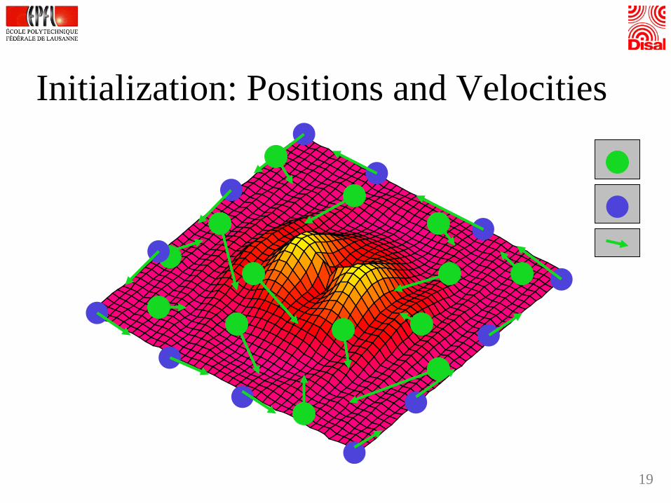
Initialization: Positions and Velocities

19

The Main PSO Loop – Parameters and Variables

• Functions– rand ()= uniformly distributed random number in [0,1]

• Parameters– w: velocity inertia (positive scalar)– cp: personal best coefficient/weight (positive scalar)– cn: neighborhood best coefficient/weight (positive scalar)

• Variables– xij(t): position of particle i in the j-th dimension at iteration t (j = [1,D])– vij(t): velocity of particle i in the j-th dimension at iteration t– : position of particle i in the j-th dimension with maximal fitness up to

iteration t (personal best)– : position of particle i’ in the j-th dimension having achieved the

maximal fitness up to iteration t in the neighborhood of particle i(neighborhood best)

)(* txij

)(* tx ji′

20

The Main PSO Loop (Eberhart, Kennedy, and Shi, 1995, 1998)

for each particle i

update the

velocity

( ) ( )1)1( ++=+ tvtxtx ijijijthen move

for each component j

At each time step t

)()()()(

)()1(**

ijjinijijp

ijij

xxrandcxxrandc

twvtv

−+−

+=+

′

21

The main PSO Loop- Vector Visualization

*ix

Here I am!

The position withoptimal fitness of my neighbors up to date

My position for optimal fitness up to date

xi

vi

*ix ′

22

Neighborhood Types• Size:

– Neighborhood index considers also the particle itself in the counting

– Local: only k neighbors considered over m particles in the population (1 < k < m); k=1 means no information from other particles used in velocity update

– Global: m neighbors• Topology:

– Indexed– Geographical– Social– Random– … 23

Neighborhood Example: Indexed and Circular (lbest)

Virtual circle

1

5

7

64

3

8 2Particle 1’s 3-

neighbourhood

24

Neighborhood Examples: Geographical vs. Social

geographical social

25

A Simple PSO Animation

© M. Clerc26

Genetic Algorithms

27

Why GA?• Reference as often compared with PSO• Older and widely spread metaheuristic technique,

pioneering work applied to robotics used GA• Originally designed for discrete optimization

problems• In this course: highly summarized description

Note: PSO is NOT an evolutionary algorithm!

Genetic Algorithms Inspiration• In natural evolution, organisms adapt to

their environments – better able to survive over time

• Aspects of evolution:– Survival of the fittest– Genetic combination in reproduction– Mutation

• Genetic Algorithms use evolutionary techniques to achieve parameter optimization and solution design

29

Algorithm Flowchart

Initialize Population

Generation loop

End criterion met?

End

Start

NY

Ex. of end criteria:

• # of generations

• best solution performance

•…30

Generation Loop

Evaluation of Individual Candidate

Solutions

Population replenishing Selection

Crossover and mutation

Decoding (genotype → phenotype)

System

Fitness measurementand encoding (phenotype

→ genotype)

Population Manager

31

GA: Basic Operators• Selection: roulette wheel (selection probability determined by

normalized fitness), ranked selection (selection probability determined by fitness order), elitist selection (highest fitness individuals always selected)

• Crossover (e.g.,1 point, pcrossover = 0.2)

• Mutation (e.g., pmutation = 0.05)

Gk Gk’

32

GA vs. PSO on Benchmark Functions

33

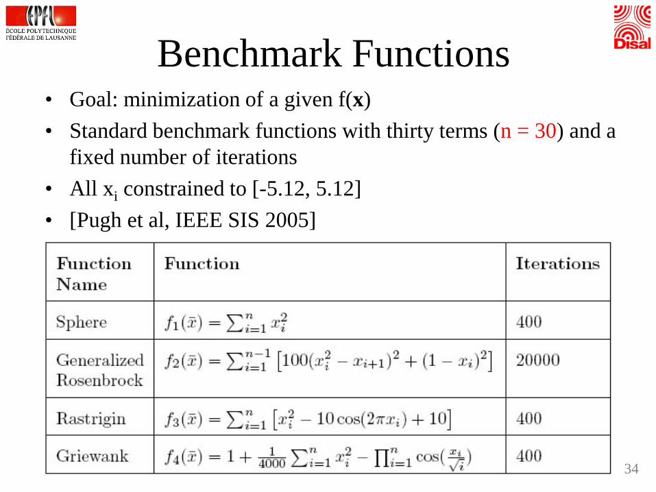
Benchmark Functions• Goal: minimization of a given f(x)• Standard benchmark functions with thirty terms (n = 30) and a

fixed number of iterations• All xi constrained to [-5.12, 5.12]• [Pugh et al, IEEE SIS 2005]

34

Benchmark functions

-2-1

01

2

-10

12

340

500

1000

1500

2000

2500

3000

-2-1

01

2

-2-1

0

120

2

4

6

8

-5

0

5

-5

0

50

20

40

60

80

100

-5

0

5

-5

0

50

0.5

1

1.5

2

2.5

Sphere Generalized Rosenbrock

Rastrigin Griewank 35

• GA: Roulette Wheel for selection, mutation applies numerical adjustment to gene

• PSO: lbest ring topology with neighborhood of size 3• Algorithm parameters used (not optimized in general):

Algorithmic Parameters

20*, 30 20*,30

36* [Pugh et al, SIS 2005]: distributed handout but biased results (small population,

limited numbers of runs)

GA vs. PSO – 20 candidate solutions

Function GA (mean ± std dev)

PSO(mean ± std dev)

Sphere 0.02 ± 0.01 0.00 ± 0.00

Generalized Rosenbrock

34.6 ± 18.9 7.38 ± 3.27

Rastrigin 157 ±21.8 48.3 ± 14.4

Griewank 0.01 ± 0.01 0.01 ± 0.03

Bold: best results; 20 runs; no noise on the performance function

37

Function GA(mean ± std dev)

PSO(mean ± std dev)

Sphere 0.01 ± 0.00 0.64 ± 0.22

Generalized Rosenbrock

37.7 ± 23.05 9.70 ± 7.23

Rastrigin 116.35 ± 26.0 105.15 ± 13.2

Griewank 0.00 ± 0.01 0.04 ± 0.02

Bold: best results; 30 runs; no noise on the performance functionGA vs. PSO – 30 candidate solutions

38Note: data different from [Pugh et al., SIS 2005]; experiments by E. Di Mario

GA vs. PSO – Overview• According to most recent research, PSO

outperforms GA on most (but not all!) continuous optimization problems

• GA still much more widely used in general research community and robust to continuous and discrete optimization problems

• Because of random aspects, very difficult to analyze either metaheuristic or make guarantees about performance

39

Design and Optimization of Obstacle Avoidance Behavior

using Genetic Algorithms

40

Evolving a Neural Controller

f(xi)

Ij

Ni

wij

1e12)( −+

= −xxf

output

synaptic weight

input

neuron N with sigmoidtransfer function f(x)

S1

S2

S3 S4S5

S6

S7S8

M1 M2

∑=

+=m

jjiji IIwx

10

Oi

)( ii xfO =

inhibitory conn.excitatory conn.

Note: In our case we evolve synaptic weigths but Hebbian rules for dynamic change of the weights, transfer function parameters, … can also be evolved (see Floreano’s course) 41

Evolving Obstacle Avoidance(Floreano and Mondada 1996)

• V = mean speed of wheels, 0 ≤ V ≤ 1• ∆v = absolute algebraic difference

between wheel speeds, 0 ≤ ∆v ≤ 1• i = activation value of the sensor with the

highest activity, 0 ≤ i ≤ 1

)1)(1( iVV −∆−=Φ

Note: Fitness accumulated during evaluation span, normalized over number of control loops (actions).

Defining performance (fitness function):

42

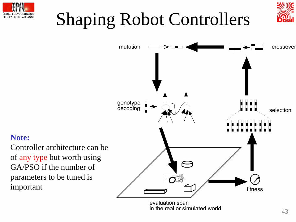
Shaping Robot Controllers

Note:Controller architecture can be of any type but worth using GA/PSO if the number of parameters to be tuned is important

43

Evolving Obstacle Avoidance

Evolved path

Fitness evolution

44

Evolved Obstacle Avoidance Behavior

Note: Direction of motion NOT encoded in the fitness function: GA automatically discovers asymmetry in the sensory system configuration (6 proximity sensors in the front and 2 in the back)

Generation 100 • on-line • off-board (PC-hosted)• hardware-in-the-loop• population-based

45

Not only Obstacle Avoidance: Evolving More

Complex Behaviors

46

Evolving Homing Behavior(Floreano and Mondada 1996)

Set-up Robot’s sensors

47

• Fitness function:

• V = mean speed of wheels, 0 ≤ V ≤ 1• i = activation value of the sensor with the

highest activity, 0 ≤ i ≤ 1

)1( iV −=Φ

• Fitness accumulated during life span, normalized over maximal number (150) of control loops (actions).

• No explicit expression of battery level/duration in the fitness function (implicit).• Chromosome length: 102 parameters (real-to-real encoding).• Generations: 240, 10 days hardware-in-the-loop evolution

Controller

Evolving Homing Behavior

48

Evolving Homing Behavior

Battery energy

Left wheel activation

Right wheel activation

Battery recharging vs. motion patterns

Reach the nest -> battery recharging -> turn on spot -> out of the nest

Evolution of # control loops per evaluation span

Fitness evolution

49

Evolved Homing Behavior

50

Not only Control Shaping: Automatic

Hardware-Software Co-Design and Optimization in Simulation and Validation

with Real Robots

51

Moving BeyondController-Only Evolution

• Evidence: Nature evolve HW and SW at the same time …

• Faithful realistic simulators enable to explore design solution which encompasses co-evolution(co-design) of control and morphological characteristics (body shape, number of sensors, placement of sensors, etc. )

• GA (PSO?) are powerful enough for this job and the methodology remain the same; only encoding changes

52

Evolving Control and Robot Morphology

(Lipson and Pollack, 2000)

http://www.mae.cornell.edu/ccsl/research/golem/index.html• Arbitrary recurrent ANN• Passive and active (linear

actuators) links• Fitness function: net distance

traveled by the centre of mass in a fixed duration

Example of evolutionary sequence: 53

Examples of Evolved Machines

Problem: simulator not enough realistic (performance higher in simulation because of not good enough simulated friction; e.g., for the arrow configuration 59.6 cm vs. 22.5 cm) 54

Issues for Evolving Real Systems by Exploiting Simulation

Goal: speeding up evolutionTraditional recipes (see Axis 2 classification): 1. Evolve in simulation, download on real HW Issue: Bridge the simulation-reality gap2. Evolve with real HW in the loop Issue: evaluation span too time consuming

(and fragile)

55

Co-Evolution of Simulation and Reality

[Bongard, Zykov, and Lipson, 2006]

http://ccsl.mae.cornell.edu/emergent_self_models 56

Morphological Estimation and Damage Recovery

[Bongard, Zykov, and Lipson, 2006]57

Co-Evolution of Models and Reality• “Analysis by synthesis” method• Powerful system identification method (not only

model parameters but also model structure)• Limitation: implies knowledge about the

underlying phenomena, shrinking the system rules to a possible alphabet (gray box as opposed to black box identification)

58

Expensive Optimization and Noise Resistance

59

Expensive Optimization Problems

1. Time for evaluation of candidate solutions (e.g., tens of seconds) >> time for application of metaheuristic operators (e.g., milliseconds)

2. Noisy performance evaluations disrupt the adaptation process and require multiple evaluations for actual performance

Two fundamental reasons making robot control design and optimization expensive in terms of time:

60

Reducing Evaluation TimeGeneral recipe: exploit more abstracted, calibrated representations (models and simulation tools)

See also multi-level modeling lectures (W8 and W9)

61

Dealing with Noisy Evaluations• Better information about candidate solution can be obtained by

combining multiple noisy evaluations• We could evaluate systematically each candidate solution for a

fixed number of times → not efficient from a computational perspective

• We want to dedicate more computational time to evaluate promising solutions and eliminate as quickly as possible the “lucky” ones

• Idea: re-evaluate and aggregate → each candidate solution might have been evaluated a different number of times → compare the aggregated value

• For instance, in GA good and robust candidate solutions survive over generations; in PSO they survive in the individual memory

• Use dedicated functions for aggregating multiple evaluations: e.g., minimum and average or more generalized aggregation functions (e.g., quasi-linear weighted means), perhaps combined with a statistical test for comparing resulting aggregated performances (see W11 lecture) 62

GA PSO

63

Testing Noise-Resistant on Benchmarks

• Benchmark 1 : Sphere and Generalized Rosenbrockfunctions– 30 real parameters [Pugh et al., SIS 2005]– Minimize objective function– Expensive only because of noise

• Benchmark 2: obstacle avoidance on a robot– 24 real parameters– Maximize objective function– Expensive because of noise and evaluation time

64

Benchmark 1: Gaussian Additive Noise on Generalized Rosenbrock

Fair test: samenumber of evaluations candidate solutions for all algorithms (i.e. N generations/ iterations of standard versions compared with N/2 of the noise-resistant ones)

65

[Pugh et al., SIS 2005]

Biased results: low number of runs (20) and population size (20) < search dimension (30)!

Increasing Noise Level – Set-Up

• Scenario 1: One robot learning obstacle avoidance

• Scenario 2: One robot learning obstacle avoidance, one robot running pre-evolved obstacle avoidance

• Scenario 3: Two robots co-learning obstacle avoidance

Idea: more robots more noise (as perceived from an individual robot) because there is no explicit communication between the robots, but in scenario 3 there is information sharing through the population manager.

1x1 m arena, PSO, 50th iteration, scenario 3

[Pugh et al, SIS 2005] 66

Increasing Noise Level – Sample Results

[Pugh et al, SIS 2005] 67

Conclusion

68

Take Home Messages• Machine-learning algorithms can be classified as supervised,

unsupervised, and reinforcement-based (evaluative)• Evaluative techniques are key for robotic learning• Two robust population-based metaheuristics are PSO and GA• PSO is a younger technique than GA but extremely promising• Evaluative techniques can be used for design and optimization of

behaviors whose complexity goes beyond obstacle avoidance• Machine-learning techniques can be also used for design and

optimization of hardware features with the help of simulation tools

• Automatic design and optimization problems in robotics are computationally expensive because of long and noisy evaluation of candidate solutions 69

Additional Literature – Week 10Books• Mitchell M., “An Introduction to Genetic Algorithms”. MIT

Press, 1996.• Kennedy J. and Eberhart R. C. with Y. Shi, “Swarm

Intelligence”. Morgan Kaufmann Publisher, 2001. • Clerc M., “Particle Swarm Optimization”. ISTE Ltd.,

London, UK, 2006.• Engelbrecht A. P., “Fundamentals of Computational Swarm

Intelligence”. John Wiley & Sons, 2006. • Nolfi S. and Floreano D., “Evolutionary Robotics: The

Biology, Intelligence, and Technology of Self-Organizing Machines”. MIT Press, 2004.

• Sutton R. S. and Barto A. G., “Reinforcement Learning: An Introduction”. The MIT Press, Cambridge, MA, 1998.

70