Distributed Learning of Distributions via Social Sampling

0018-9286 (c) 2013 IEEE. Personal use is permitted, but republication/redistribution requires IEEE permission. Seehttp://www.ieee.org/publications_standards/publications/rights/index.html for more information.

This article has been accepted for publication in a future issue of this journal, but has not been fully edited. Content may change prior to final publication. Citation information: DOI10.1109/TAC.2014.2329611, IEEE Transactions on Automatic Control

1

Distributed Learning of Distributions via SocialSampling

Anand D. Sarwate, Member, IEEE, and Tara Javidi, Senior Member, IEEE,

Abstract—A protocol for distributed estimation of discretedistributions is proposed. Each agent begins with a single samplefrom the distribution, and the goal is to learn the empiricaldistribution of the samples. The protocol is based on a simplemessage-passing model motivated by communication in socialnetworks. Agents sample a message randomly from their currentestimates of the distribution, resulting in a protocol with quan-tized messages. Using tools from stochastic approximation, thealgorithm is shown to converge almost surely. Examples illustratethree regimes with different consensus phenomena. Simulationsdemonstrate this convergence and give some insight into the effectof network topology.

I. INTRODUCTION

The emergence of large-network paradigms for commu-nications and the widespread adoption of social networkingtechnologies has resurrected interest in classical models ofopinion formation and distributed computation as well as newapproaches to distributed learning and inference. In this paperwe propose a simple message passing protocol inspired bysocial communication and show how it allows a network ofindividuals can learn about global phenomena. In particular,we study a situation wherein each node or agent in a networkholds an initial opinion and the agents communicate witheach other to infer the distribution of their initial opinions.Our model of messaging is a simple abstraction of socialcommunication in which individuals exchange single opinions.This model is a randomized approximation of consensusprocedures. Because agents collect samples of the opinionsof their neighbors, we call our model social sampling.

In our protocol agents merge the sampled opinions of theirneighbors with their own estimates using a weighted average.

Manuscript received May 17, 2013; revised January 9, 2014; secondrevision . Date of current version June 5, 2014. The work of both authorswas funded by National Science Foundation (NSF) Grant Number CCF-1218331. A.D. Sarwate received additional support from the CaliforniaInstitute for Telecommunications and Information Technology (CALIT2)at UC San Diego. T. Javidi received additional support from NSF GrantNumbers CCF-1018722 and CNS-1329819. Simulations were supported bythe UCSD FWGrid Project, NSF Research Infrastructure Grant Number EIA-0303622. Parts of this work were presented at the 46th Annual Conferenceon Information Sciences and Systems (CISS), Princeton, NJ, USA, March2012 [1], and the 49th Annual Allerton Conference on Communication,Control and Computation, Monticello, IL, USA, September 2011 [2].

Anand D. Sarwate is with the Department of Electrical and ComputerEngineering, Rutgers, The State University of New Jersey, 84 Brett Road,Piscataway, NJ 08854, USA. Email: [email protected]. TaraJavidi is with the Department of Electrical and Computer Engineering,University of California, San Diego, 9500 Gilman Dr. MC 0407, La JollaCA 92093-0407, USA. Email: [email protected].

Communicated by xxxxxxxxxx.Digital Object Identifier xxxxxxxxxxxxCopyright (c) 2014 IEEE. Personal use of this material is permitted. How-

ever, permission to use this material for any other purposes must be obtainedfrom the IEEE by sending a request to [email protected].

Averaging has been used to model opinion formation fordecades, starting with the early work of French [3], Harary[4], and DeGroot [5]. These works focused on averaging as ameans to an end – averaging the local opinions of a group ofpeers was a simple way to model the process of negotiationand compromise of opinions represented as scalar variables.A natural extension of the above work is that where all agentsare interested in the local reconstruction of the empiricaldistribution of discrete opinions. Such locally constructedempirical distributions not only provide richer informationabout global network properties (such as the outcome of avote, the confidence interval around the mean, etc), but froma statistical estimation perspective provide estimates of localsufficient statistics when the agents’ opinions are independentand identically distributed (i.i.d.) samples from a commondistribution.

For opinions taking value in a finite, discrete set, wecan compute the empirical distribution of opinions across anetwork by running an average consensus algorithm for eachpossible value of the opinion. This can even be done in parallelso that at each time agents exchange their entire histogram ofopinions and compute weighted averages of their neighbors’histograms to update their estimate. In a social network, thiswould correspond to modeling the interaction of two agents asa complete exchange of their entire beliefs in every opinion,which is not realistic. In particular, if the number of possibleopinions is large (corresponding to a large number of bins orelements in the histogram), communicating information aboutall opinions may be very inefficient, especially if the truedistribution of opinions is far from uniform.

In contrast, this paper considers a novel model in whichagents’ information is disseminated through randomly selectedsamples of locally constructed histograms [2]. The use ofrandom samples results in a much lower overhead becauseit accounts for the popularity/frequency of histogram binsand naturally enables finite-precision communication amongneighboring nodes. It is not hard to guarantee that the ex-pectation of the node estimates converges to the true his-togram when the mean of any given (randomized and noisy)shared sample is exactly the local estimate of the histogram.However, to ensure convergence in an almost sure sense weuse techniques from stochastic approximation. We identifythree interesting regimes of behavior. In the first, studied byNarayanan and Niyogi [6], agents converge to atomic distri-butions on a common single opinion. In the second, agentsconverge to a common consensus estimate which in generalis not equal to the true histogram. Finally, we demonstrate arandomized protocol which, under mild technical assumptions,ensures convergence of agents’ local estimates to the global

Limited circulation. For review only

Preprint submitted to IEEE Transactions on Automatic Control. Received: June 5, 2014 06:45:10 PST



2

histogram almost surely. The stochastic approximation pointof view suggests that a set of decaying weights can controlthe accumulation of noise along time and still compute theaverage histogram.

Related work

In addition to the work in mathematical modeling of opinionformation [3]–[5], there has been a large body of work on con-sensus in terms of decision making initiated by Aumann [7].Borkar and Varaiya [8] studied distributed agreement protocolsin which agents are trying to estimate a common parameter.The agents randomly broadcast conditional expectations basedon all of the information they have seen so far, and they findgeneral conditions under which the agents would reach anasymptotic agreement. If the network is sufficiently connected(in a certain sense), the estimates converge to the centralizedestimate of the parameter, even when the agents’ memoryis limited [9]. In these works the questions are more aboutwhether agreement is possible at all, given the probabilitystructure of the observation and communication.

There is a significant body of work on consensus andinformation aggregation in sensor networks [10]–[18]. Fromthe protocol perspective, many authors have studied the effectof network topology on the rate of convergence of consensusprotocols [10]–[12], [16]–[21]. For communication networksthe speed can be accelerated by exploiting network properties[22]–[25] (see surveys in [19], [26] for more references).Others have studied how quantization constraints impact con-vergence [27]–[34]. However, in all of these works the agentsare assumed to be some sort of computational devices likerobotic networks or sensor networks. A comprehensive viewof this topic is beyond the scope of this paper. Instead,we focus on a few papers most relevant to our model andstudy: consensus with quantized messages and consensus viastochastic approximation. However, it is important to notethat in contrast to all the studies discussed below, our workprimarily deals with an extension of the classic consensus(linear combination of private values) in that we are inter-ested in ensuring agreement over the space of distributions(histograms).

Our goal in this paper is to ensure the convergence of eachagent’s local estimate to a true and global discrete distributionvia a low-overhead algorithm in which messages are chosenin a discrete set. Our work is therefore related to the extensiverecent literature on quantized consensus [28], [30], [31], [33].In these works, as in ours, the communication between nodesis discretized (and in some cases the storage/computationat nodes as well [30]) and the question is how to ensureconsensus (within a bin) to the average. This is in sharpcontrast to our model which uses discrete messages to con-vey and ensure consensus on the network-wide histogram ofdiscrete values. As a result, in contrast to the prior work onquantization noise [27], [31], [35], the “noise” is manufacturedby our randomized sample selection scheme and hence playsa significantly different role.

Our analysis uses similar tools from stochastic approxima-tion as recent studies of consensus protocols [34], [36], [37].

However, these works use stochastic approximation to addressthe effect of random noise in network topology, messagetransmission, and computation for a scalar consensus problem,while our use of standard theorems in stochastic approximationis to handle the impact of the noise that comes from thesampling scheme that generates our random messages. In otherwords, our noise is introduced by design even though ourtechnique to control its cumulative effect is similar.

II. MODEL AND ALGORITHMS

Let [n] denote the set {1, 2, . . . , n} and let ei ∈ RM denotethe i-th elementary row vector in which the i-th coordinate is1 and all other coordinates are 0. Let 1(·) denote the indicatorfunction and 1 the column vector whose elements are all equalto 1. Let ‖·‖ denote the Euclidean norm for vectors and theFrobenius norm for matrices. We will represent probabilitydistributions on finite sets as row vectors, and denote the setof probability distributions on a countable set A by P(A).

A. Problem setup

Time is discrete and indexed by t ∈ {0, 1, 2, . . .}. Thesystem contains n agents or “nodes.” At time t the agentscan communicate with each other according to an undirectedgraph G(t) with vertex set [n] and edge set E(t). Let Ni(t) ={j : (i, j) ∈ E(t)} be the set of neighbors of node i. If(i, j) ∈ E(t) then nodes i and j can communicate at timet. Let G(t) denote the adjacency matrix of G(t) and let D(t)be the diagonal matrix of node degrees. The Laplacian of G(t)is L(t) = D(t)−G(t).

At time 0 every node starts with a single discrete sampleXi ∈ X = [M ]. The goal of the network is for each node toestimate the empirical distribution, or normalized histogram,of the observations {Xi : i ∈ [n]}:

Π(x) =1

n

n∑i=1

1(Xi = x) · ex ∀x ∈ [M ].

To make it simpler to characterize the overall communica-tion overhead, we assume that• Agents can exchange messages Yi(t) lying in a finite setY .

• At each time t = 1, 2, . . . agents can transmit a singlemessage to all of their neighbors.

At each time t = 0, 1, 2, . . ., each node i maintains an internalestimate Qi(t) of the distribution Π, and we take Qi(0) = eXi .Every node i generates its message Yi(t) ∈ Y as a function ofthis internal estimate Qi(t). Furthermore, each node i receivesthe messages {Yj(t) : j ∈ Ni} from its neighbors and usethese messages to perform an update of its estimate Qi(t+ 1)using Qi(t), {Yj(t) : j ∈ Ni}.

Since in a single time t there are potentially 2|E(t)| mes-sages transmitted in the network, a first approximation for thecommunication overhead of this class of schemes is simplyproportional to the number of edges in the network multipliedby the logarithm of the cardinality of set Y .

We are interested in the properties of the estimates Qi(t) ast→∞. In particular, we are interested in the case where every





3

element in the set {Qi(t) : i ∈ n} converges almost surely to acommon random variable q∗. In this case, we call the randomvector q∗ the consensus variable. Different algorithms that weconsider will result in different properties of this consensusvariable. For example, the we will consider the support of thedistribution of q∗ as well as its expectation.

B. Social sampling and linear updates

In this paper we assume that Y = {0, e1, e1, . . . eM},with the convention that node i transmits nothing (or remainssilent) when Yi(t) = 0. Furthermore, we consider the class ofschemes where the random message Yi(t) ∈ Y of node i attime t is generated according to a distribution Pi(t) ∈ P(Y)which itself is a function of the estimate Qi(t). In otherwords, Pi(t) is a row vector of length M where P(Yi(t) =em) = Pi,m(t). We frequently refer to the random messagesYi(t) ∈ Y, i ∈ [n], t = 0, 1, . . . as social samples becausethey correspond to nodes obtaining random samples of theirneighbor’s opinions. Note that although the random variableYi(t) takes values in RM , it is supported only on the finite setY and hence requires communicating log |Y| information bits.

For simplicity in this paper, we often rely on matrixrepresentation across the network. Accordingly, let Y(t) bethe n × M matrix whose i-th row is Yi(t). Then we haveE[Y(t)] = P(t).

Let {W (t) : t = 0, 1, 2, . . .} be a sequence of n×n matriceswith nonnegative entries, such that Wij(t) = 0 for all (i, j) 6=E(t). We study linear updates of the form

Qi(t+ 1) = (1− δ(t)Aii(t))Qi(t)− δ(t)Bii(t)Yi(t)

+∑

j∈Ni(t)

δ(t)Wij(t)Yj(t). (1)

Here the parameter δ(t) is a step size for the algorithm. LetQ(t) be the n ×M matrix whose i-th row is Qi(t). We canwrite the iterates more compactly as

Q(t+ 1) = (I − δ(t)A(t))Q(t)− δ(t)B(t)Y(t)

+ δ(t)W (t)Y(t),

where A(t) and B(t) are diagonal matrices.In the next section we will analyze this update and identify

conditions under which the estimates Qi(t) converge to acommon q∗ ∈ P(Y) and additional conditions under whichq∗ = Π. To provide a unified analysis of these differentalgorithms, we transform the update equation into a stochasticiteration

Q(t+ 1) = Q(t) + δ(t)[H(t)Q(t) + C(t) + M(t)

]. (2)

In this form of the update, the matrix H(t) represents themean effect of the network connectivity, M(t) is a martingaledifference term related to the randomness in the networktopology and social sampling, and C(t) is a correction termassociated with the difference between the estimate Q(t) andthe sampling distribution P(t).

Lemma 1. The iteration in (1) can be rewritten as (2), where

H(t)4= W (t)− B(t)− A(t) (3)

C(t)4= (W (t)−B(t)) (P(t)−Q(t))

+(W (t)−B(t)− W (t) + B(t)

)Y(t) (4)

M(t)4=(W (t)−B(t)−A(t)− W (t) + B(t) + A(t)

)Q(t)

+(W (t)− B(t)

)(Y(t)−P(t))

+(W (t)− B(t)−W (t) +B(t)

)P(t). (5)

and the term M(t) is a martingale difference sequence:

E[M(t)|Ft] = 0.

Proof. Rewriting the iterates, we see that

Q(t+ 1) = Q(t) + δ(t)[−A(t)Q(t)

+ (W (t)−B(t))Y(t)], (6)

and the term multiplied by δ(t) can be expanded:

−A(t)Q(t)+(W (t)−B(t))Y(t)

=(W (t)− B(t)− A(t)

)Q(t)

+(W (t)−B(t)−A(t)

− W (t) + B(t) + A(t))Q(t)

+ (W (t)−B(t)) (Y(t)−Q(t))

=(W (t)− B(t)− A(t)

)Q(t)

+(W (t)−B(t)−A(t)

− W (t) + B(t) + A(t))Q(t)

+ (W (t)−B(t)) (P(t)−Q(t))

+ (W (t)−B(t)) (Y(t)−P(t))

=(W (t)− B(t)− A(t)

)Q(t)

+(W (t)−B(t)−A(t)

− W (t) + B(t) + A(t))Q(t)

+ (W (t)−B(t)) (P(t)−Q(t))

+(W (t)− B(t)

)(Y(t)−P(t))

+(W (t)− B(t)−W (t) +B(t)

)P(t)

+(W (t)−B(t)− W (t) + B(t)

)Y(t)

]. (7)

Define H , C, and M(t) as in (3), (4) and (5). Furthermore,define

M(t) =(W (t)−B(t)−A(t)

− W (t) + B(t) + A(t))Q(t)

+(W (t)− B(t)

)(Y(t)−P(t))

+(W (t)− B(t)−W (t) +B(t)

)P(t).

Taking conditional expectation of both sides of (6) and notingthat E[Y(t)|Ft] = P(t), we have the result.

Loosely speaking, the term C(t) will be asymptoticallyvanishing if P(t) → Q(t) and the matrices W (t) and B(t)are asymptotically independent of Y(t). In the next section,we show that this stochastic approximation scheme convergesunder certain conditions on update rule.





4

0.00

0.25

0.50

0.75

1.00

0 50 100 150time

Nod

e es

timat

e elementQ1Q2Q3Q4

Estimate at a single node vs. time

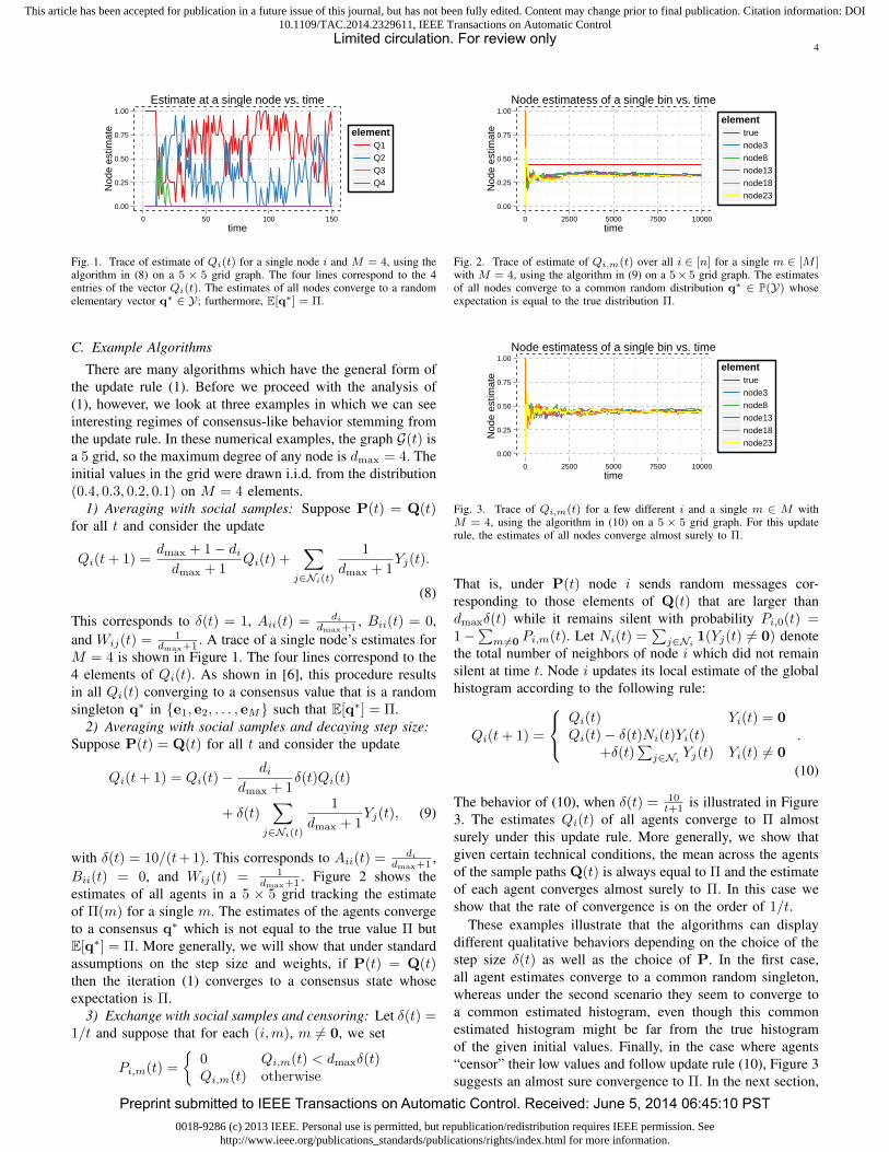
Fig. 1. Trace of estimate of Qi(t) for a single node i and M = 4, using thealgorithm in (8) on a 5 × 5 grid graph. The four lines correspond to the 4entries of the vector Qi(t). The estimates of all nodes converge to a randomelementary vector q∗ ∈ Y; furthermore, E[q∗] = Π.

C. Example Algorithms

There are many algorithms which have the general form ofthe update rule (1). Before we proceed with the analysis of(1), however, we look at three examples in which we can seeinteresting regimes of consensus-like behavior stemming fromthe update rule. In these numerical examples, the graph G(t) isa 5 grid, so the maximum degree of any node is dmax = 4. Theinitial values in the grid were drawn i.i.d. from the distribution(0.4, 0.3, 0.2, 0.1) on M = 4 elements.

1) Averaging with social samples: Suppose P(t) = Q(t)for all t and consider the update

Qi(t+ 1) =dmax + 1− didmax + 1

Qi(t) +∑

j∈Ni(t)

1

dmax + 1Yj(t).

(8)

This corresponds to δ(t) = 1, Aii(t) = didmax+1 , Bii(t) = 0,

and Wij(t) = 1dmax+1 . A trace of a single node’s estimates for

M = 4 is shown in Figure 1. The four lines correspond to the4 elements of Qi(t). As shown in [6], this procedure resultsin all Qi(t) converging to a consensus value that is a randomsingleton q∗ in {e1, e2, . . . , eM} such that E[q∗] = Π.

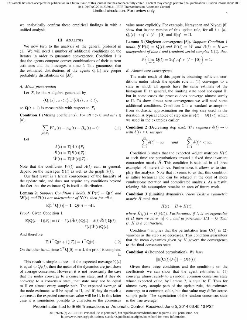
2) Averaging with social samples and decaying step size:Suppose P(t) = Q(t) for all t and consider the update

Qi(t+ 1) = Qi(t)−di

dmax + 1δ(t)Qi(t)

+ δ(t)∑

j∈Ni(t)

1

dmax + 1Yj(t), (9)

with δ(t) = 10/(t+ 1). This corresponds to Aii(t) = didmax+1 ,

Bii(t) = 0, and Wij(t) = 1dmax+1 . Figure 2 shows the

estimates of all agents in a 5 × 5 grid tracking the estimateof Π(m) for a single m. The estimates of the agents convergeto a consensus q∗ which is not equal to the true value Π butE[q∗] = Π. More generally, we will show that under standardassumptions on the step size and weights, if P(t) = Q(t)then the iteration (1) converges to a consensus state whoseexpectation is Π.

3) Exchange with social samples and censoring: Let δ(t) =1/t and suppose that for each (i,m), m 6= 0, we set

Pi,m(t) =

{0 Qi,m(t) < dmaxδ(t)Qi,m(t) otherwise

0.00

0.25

0.50

0.75

1.00

0 2500 5000 7500 10000time

Nod

e es

timat

e

elementtruenode3node8node13node18node23

Node estimatess of a single bin vs. time

Fig. 2. Trace of estimate of Qi,m(t) over all i ∈ [n] for a single m ∈ [M ]with M = 4, using the algorithm in (9) on a 5× 5 grid graph. The estimatesof all nodes converge to a common random distribution q∗ ∈ P(Y) whoseexpectation is equal to the true distribution Π.

0.00

0.25

0.50

0.75

1.00

0 2500 5000 7500 10000time

Nod

e es

timat

e

elementtruenode3node8node13node18node23

Node estimatess of a single bin vs. time

Fig. 3. Trace of Qi,m(t) for a few different i and a single m ∈ M withM = 4, using the algorithm in (10) on a 5 × 5 grid graph. For this updaterule, the estimates of all nodes converge almost surely to Π.

That is, under P(t) node i sends random messages cor-responding to those elements of Q(t) that are larger thandmaxδ(t) while it remains silent with probability Pi,0(t) =1−

∑m 6=0 Pi,m(t). Let Ni(t) =

∑j∈Ni

1(Yj(t) 6= 0) denotethe total number of neighbors of node i which did not remainsilent at time t. Node i updates its local estimate of the globalhistogram according to the following rule:

Qi(t+ 1) =

Qi(t) Yi(t) = 0Qi(t)− δ(t)Ni(t)Yi(t)

+δ(t)∑j∈Ni

Yj(t) Yi(t) 6= 0.

(10)

The behavior of (10), when δ(t) = 10t+1 is illustrated in Figure

3. The estimates Qi(t) of all agents converge to Π almostsurely under this update rule. More generally, we show thatgiven certain technical conditions, the mean across the agentsof the sample paths Q(t) is always equal to Π and the estimateof each agent converges almost surely to Π. In this case weshow that the rate of convergence is on the order of 1/t.

These examples illustrate that the algorithms can displaydifferent qualitative behaviors depending on the choice of thestep size δ(t) as well as the choice of P. In the first case,all agent estimates converge to a common random singleton,whereas under the second scenario they seem to converge toa common estimated histogram, even though this commonestimated histogram might be far from the true histogramof the given initial values. Finally, in the case where agents“censor” their low values and follow update rule (10), Figure 3suggests an almost sure convergence to Π. In the next section,





5

we analytically confirm these empirical findings in with aunified analysis.

III. ANALYSIS

We now turn to the analysis of the general protocol in(1). We will need a number of additional conditions on theiterates in order to guarantee convergence. Condition 1 isthat the agents compute convex combinations of their currentestimates and the messages at time t. This guarantees thatthe estimated distributions of the agents Qi(t) are properprobability distributions on [M ].

A. Mean preservation

Let Ft be the σ-algebra generated by

{Qi(s) : s < t} ∪ {G(s) : s < t},

so Q(t+ 1) is measurable with respect to Ft.

Condition 1 (Mixing coefficients). For all t > 0 and all i ∈[n], ∑

j∈Ni

Wij(t)−Aii(t)−Bii(t) = 0. (11)

Let

A(t) = E[A(t)|Ft]B(t) = E[B(t)|Ft]W (t) = E[W (t)|Ft].

Note that the coefficient W (t) and A(t) can, in general,depend on the messages Y(t) as well as the graph G(t).

Our first result is a trivial consequence of the linearity ofthe update rule, and does not require any conditions beyondthe fact that the estimate Q is itself a distribution.

Lemma 2. Suppose Condition 1 holds. If P(t) = Q(t) andW(t) and B(t) are independent of Y(t), then for all t,

E[1>Q(t)] = 1>Q(0) = nΠ.

Proof. Given Condition 1,

E[Q(t+ 1)|Ft] = (I − δ(t)A(t))Q(t)− δ(t)B(t)Q(t)

+ δ(t)W (t)Q(t).

And therefore

E[1>Q(t+ 1)|Ft] = 1>Q(t). (12)

On the other hand, since 1>Q(0) = nΠ, the proof is complete.

This result is simple to see – if the expected message Yi(t)is equal to Qi(t), then the mean of the dynamics are just thoseof average consensus. However, it is not necessarily the casethat the nodes converge to a consensus state, and if they doconverge to a consensus state, that state may not be equalto Π on almost every sample path. The expected average ofthe node estimates will be equal to Π, and if they do reach aconsensus the expected consensus value will be Π. In this lattercase it is sometimes possible to characterize the consensus

value more explicitly. For example, Narayanan and Niyogi [6]show that in one version of this update rule, for all i ∈ [n],Qi(t)→ q∗ ∈ Y − {0} and E[q∗] = Π.

Lemma 3 (Singleton convergence [6]). Suppose Condition 1holds. If P(t) = Q(t) and W (t) = W and B(t) = B areindependent of time t and (random) social samples Y(t), then

P{

limt→∞

Q(t) = 1q∗,q∗ ∈ Y − {0}}

= 1.

B. Almost sure convergence

The main result of this paper is obtaining sufficient con-ditions under which the update rule in (1) converges to astate in which all agents have the same estimate of thehistogram Π. In general, the limiting state need not equal Π,but in some cases the process does converge almost surelyto Π. To show almost sure convergence we will need someadditional conditions. Condition 2 is a standard assumptionfrom stochastic approximation on the step size used in theiteration. A typical choice of step size is δ(t) = Θ(1/t) whichwe used in the examples earlier.

Condition 2 (Decreasing step size). The sequence δ(t) → 0with δ(t) ≥ 0 satisfies

∞∑t=1

δ(t) =∞ and∞∑t=1

δ(t)2 <∞.

Condition 3 states that the expected weight matrices H(t)at each time are perturbations around a fixed time-invariantcontraction matrix H . This condition is satisfied in all threeexamples of interest above. Furthermore, it allows us to sim-plify the analysis. Note that it seems to us that this conditionis rather technical and can be relaxed at the cost of morecumbersome notation and complicated analysis. As a result,relaxing this assumption remains an area of future work.

Condition 3 (Limiting dynamics). There exists a symmetricmatrix H such that

H(t) = H + H(t),

where Hij(t) = O(δ(t)). Furthermore, if λ is an eigenvalueof H then we have |λ| < 1 and in particular H1 = 0. Thatis, H is a contraction.

Condition 4 implies that the perturbation term C(t) in (2)vanishes as the step size decreases. This condition guaranteesthat the mean dynamics given by H govern the convergenceto the final consensus state.

Condition 4 (Bounded perturbation). We have

‖E[C(t)|Ft]‖ = O(δ(t)).

Given these three conditions and the conditions on thecoefficients we can show that the agent estimates in (1)converge almost surely to a random common consensus statewhose expected value, by Lemma 2, is equal to Π. Thus foralmost every sample path of the update rule, the estimatesconverge to a common value, but that value may differ acrosssample paths. The expectation of the random consensus stateis the true average.





6

Theorem 1. Suppose Conditions 1, 2, 3, and 4 hold. Thenthe estimate of each node i governed by the update rule (1)converges almost surely to a random variable q∗ ∈ P(Y)which is a consensus state. That is, Q(t)→ Q∗ = 1q∗ whereE[Q∗] = 1Π.

Proof. The result follows from a general convergence theoremfor stochastic approximation algorithms [38, Theorem 5.2.1].Define

V(t) = H(t)Q(t) + C(t) + M(t).

Several additional conditions are needed to guarantee proper-ties of V(t) which ensure convergence of the update in (2).Condition 2 guarantees that the step sizes decay slowly enoughto take advantage of the almost sure convergence of stochasticapproximation procedures. The limit point is a fixed point ofthe matrix map H and Conditions 1 and 3 show that this mapis a contraction so the limit points are consensus states. Thefinal condition is that the noise in the updates can be “averagedout.” This follows in part because the process is bounded, andin part because Condition 4 shows that the perturbation mustbe decaying sufficiently fast.

We must verify a number of conditions [38, p.126] to usethis theorem.

1) Condition 2 shows that the step sizes not summable butare square summable [38, (5.1.1) and (A2.4)].

2) The iterates are bounded in the sense thatsupt E[‖V(t)‖2] < ∞. This follows because Qi(t) isa probability distribution for all t, so the updates mustalso be bounded [38, (A2.1)].

3) If we take the expected update

E[V(t)|Ft] = H(t)Q(t) + E[C(t)|Ft]= HQ(t) + H(t)Q(t) + E[C(t)|Ft],

so we can write this conditional expectation as thesum of a measurable function HQ(t) and a randomyet diminishing perturbation H(t)Q(t) + E[C(t)|Ft].Furthermore, from Condition 3, the map H is contin-uous [38, (A2.2)-(A2.3)].

4) The final thing to check [38, (A2.5)] is that the randomperturbation in the expected update decays sufficientlyquickly:∞∑t=1

δ(t)∥∥∥H(t)Q(t) + E[C(t)|Ft]

∥∥∥≤∞∑t=1

δ(t)∥∥∥H(t)

∥∥∥ ‖Q(t)‖+

∞∑t=1

δ(t) ‖E[C(t)|Ft]‖

<∞.

The last step follows from Conditions 2 and 4 as wellas boundedness of Q(t).

Applying Theorem 5.2.1 of Kushner and Yin [38] shows thatthe estimates converge to a limit set of the linear map H .Furthermore, from Condition 3 we know H is a contractionwith a single eigenvector at 1. In other words, the limit pointsare of the form Q∗ = 1q∗ where every row is identical.

The preceding theorem shows that the updates convergealmost surely to a limit when the step sizes are decreasing,

even though as shown in [6], we know that decreasing stepsize is not necessary for almost sure convergence. So far thealgorithm has no provable advantage to that of [6], in thateach node’s estimate converges to a consensus state q∗, butq∗ need not equal Π. However, by ensuring that the samplepath of the algorithm is “mean preserving” (the sum of thej-th components of all Qi(t)’s is equal to Πj), this consensuslimit becomes equal to Π.

Condition 5 (Mean preservation). The average of the nodeestimates is Π

1>Q(t) = Π ∀t.

Corollary 1. Suppose Conditions 1, 2, 3, 4, and 5 hold. ThenQ(t)→ Q∗ almost surely, where Q∗ = 1Π almost surely.

C. Rate of convergence

We now turn to bounds on the expected squared error of inthe case where Q(t)→ Q∗ almost surely.

Theorem 2 (Rate of convergence). Suppose that Conditions1, 2, 3, and 4 also hold. Then there exists a constant C suchthat

E[‖Q(t)−Q∗‖2

]≤ Cδ(t).

Proof. First note that in the process (1), Qi(t) is a probabilitydistribution, so the entire process lies in a bounded compactset, and under Conditions 3 and 4 we can write the iterationas

Q(t+ 1) = Q(t) + δ(t)[HQ(t) + D(t) + M(t)

],

where the perturbation term ‖E[D(t)|Ft]‖ = O(δ(t)). We cannow apply Theorem 24 of Benveniste et al. [39, p. 246], whichrequires checking similar conditions as the previous Theorem.

1) Condition 2 shows the step sizes are not summable [39,(A.1)].

2) Treat the tuple of random variables(A(t),B(t),W(t),Y(t)) as a state variable S(t).This state is measurable with respect to Ft, andthere exists a conditional probability distributioncorresponding to the update [39, (A.2)].

3) LetN(t) = M(t) + C(t)− E[D(t)|Ft],

so N(t) is still a martingale difference. If we defineJ(t) = 1

δ(t)E[C(t)|Ft] we can rewrite the iterates as

Q(t+ 1) = Q(t) + δ(t)[HQ(t) + N(t)

]+ δ(t)2J(t).

Again, the terms∥∥HQ(t) + N(t)

∥∥ and ‖J(t)‖ arebounded by a constant [39, (A.3) and (A.5)].

4) Since H is a linear contraction, it is also Lipschitz,and the martingale difference N(t) is bounded, whichimplies condition (A.4) of Benveniste et al. [39, p. 216].

With the validity of the above conditions , the assertion of thetheorem follows directly [39, p. 216]:

E[‖Q(t)−Q∗‖2

]= O(δ(t)).





7

D. Example Algorithms Revisited

We can now describe how the results apply to the algorithmsdescribed in section II-C.

1) Averaging with social samples: Our first algorithm in (8)was one in which the nodes perform a weighted average ofthe distribution of the messages they receive with their currentestimate. The general form of the algorithm was

Q(t+ 1) = (I −A)Q(t) +WY(t),

which corresponds to choosing δ(t) = 1 and B(t) = 0. For thespecific example in (8), A = 1

dmax+1D and W = 1dmax+1G,

where G is the adjacency matrix of the graph and D is thediagonal matrix of degrees. Furthermore, P(t) = Q(t) for allt.

Q(t+ 1) = Q(t) + (W −A)Q(t) +W (Y(t)−Q(t)).(13)

The term W − A is the graph Laplacian of the graph withedge weights given by W . The following is is a corollary ofLemma 2 and Lemma 3.

Corollary 2. For the update given in (13), the estimates Q→Q∗ almost surely, where Q∗ is a random matrix taking valuesin the set {1q∗ : q∗ ∈ Y} such that E[Q∗] = 1Π.

Examining (13), we see that the the Laplacian term drivesthe iteration to a consensus state, but the only stable consensusstates are those for which Y(t)−Q(t) = 0, which means Y(t)must be equal to Q(t) almost surely. This means each row ofQ(t) must correspond to a degenerate distribution of the formem.

2) Averaging with social samples and decaying step size:The second class of algorithms, exemplified by (9), has thefollowing general form:

Q(t+ 1) = (1− δ(t)A)Q(t) + δ(t)WY(t),

and again P(t) = Q(t) for all t. This is really the same as(13) but with a decaying step size δ(t):

Q(t+ 1) = Q(t) + δ(t)(W −A)Q(t)

+ δ(t)W (Y(t)−Q(t)). (14)

However, the existence of a decreasing step size means that theiterates under this update behave significantly differently thanthose governed by (13). The convergence of this algorithm ischaracterized by Theorems 1 and 2.

Corollary 3. For the update given in (14) with δ(t) = 1/t, theestimates Q(t) → Q∗ almost surely, where Q∗ is a randommatrix in the set {1q> : ‖q‖1 = 1, qm > 0} and E[Q∗] =

1Π>. Furthermore, E[‖Q(t)−Q∗‖2] = O(1/t).

3) Exchange with social samples and censoring: The lastalgorithm in (10) has a more complex update rule, but it is aspecial case of the generic update

Q(t+ 1) = Q(t)− δ(t)B(t)Y(t) + δ(t)W (t)Y(t). (15)

For a fixed weight matrix W , define the the thresholds ∆(t) =δ(t)

∑j∈Ni

Wij and the sampling distribution Pi,m(t) =1(Qi,m(t) > ∆(t)). The social samples Y(t) are sampled

according to this distribution and the weight matrices aredefined by

Wij(t) =

{0 i 6= j, Yi = 0 or Yi 6= 0Wij i 6= j, Yi = 0 and Yi 6= 0

Bii(t) =∑j∈Ni

Wij(t)

In this algorithm the iterates keep∑iQi,m(t) constant over

time by changing the sampling distribution P(t) over timeand by using the weight matrix B(t) to implement a “massexchange” policy between nodes. At each time, agent i sam-ples a opinion Zi(t). If Qi,Zi(t)(t) is large enough, the agentsends Yi(t) = Zi(t), giving δ(t)Wij mass to each neighbor jand subtracting the corresponding mass from its own opinion.If Qi,Zi(t)(t) is not large enough it exchanges nothing with itsneighbors. The distribution P(t) implements this “censoring”operation. By keeping the total sum on each opinion fixed,Corollary 1 shows that the estimates converge almost surelyto Π.

Corollary 4. For the update given in (15) with δ = 1/t, theestimates Q(t)→ 1Π almost surely, and E[‖Q(t)− 1Π‖2] =O(1/t).

IV. EMPIRICAL RESULTS

The preceding analysis shows the almost-sure convergenceof all node estimates for some social sampling strategies, andin some cases characterizes the rate of convergence. However,the analysis does not capture the effect of problem parameterssuch as the initial distribution of node values and the networktopology. These factors are well known to affect the rate ofconvergence of many distributed estimation and consensusprocedures – in this section we provide some empirical resultsabout these effects.

We considered a number of different topologies for oursimulations:• The

√n×√n grid has vertex set [

√n]× [

√n] and edge

exists between two nodes whose L1 distance is 1.• A star network has a single central vertex which is

connected by a single edge to n− 1 other vertices.• An Erdos-Renyi graph [40] on vertex set [n] contains each

edge (i, j) independently with probability p. We choosep = 0.6.

• A preferential attachment graph [41], [42] is constructedby adding vertices one at a time. A new vertex isconnected to an existing vertex with a probability thatis a function of the current degree of the vertices. Weallowed each new vertex to be connected to 3 precedingvertices.

• A 2-dimensional Watts-Strogatz graph is a grid withrandomly “rewired” edges [43]. We chose rewiring prob-ability 0.1.

Details on the random graph models can be found in theigraph package for the R statistical programming lan-guage [44]. In the simulations we calculated the average of1n ‖Q(t)− 1Π‖2 across runs of the simulation, which is theaverage mean-squared-error (MSE) per node of the estimates.





8

−2

−1

0

0 25000 50000 75000 100000iterations

log

MS

EStepsize

0.0001

0.01

1/t

1/t^2

Error vs. time for different step sizes(Grid)

(a) Grid

−4

−3

−2

−1

0

0 25000 50000 75000 100000iterations

log

MS

E

Stepsize

0.0001

0.01

1/t

1/t^2

Error vs. time for different step sizes(Preferential Attachment)

(b) Preferential Attachment

−4

−3

−2

−1

0

0 25000 50000 75000 100000iterations

log

MS

E

Stepsize

0.0001

0.01

1/t

1/t^2

Error vs. time for different step sizes(Watts−Strogatz)

(c) Watts-Strogatz

−4

−3

−2

−1

0

0 25000 50000 75000 100000iterations

log

MS

E

Stepsize

0.0001

0.01

1/t

1/t^2

Error vs. time for different step sizes(Star)

(d) Star

Fig. 4. Average MSE between the agent estimates and the true histogram initial node values versus time for 4 different 100-node graphs : a 10× 10 grid,preferential attachment graphs with three edges generated per new node, Watts-Strogatz graphs with rewiring probability 0.1, and a star with one central nodeand 99 peripheral nodes.

A. Network size and topology

We were interested in finding how the convergence timedepends on the step size and network topology. To investigatethis we simulated the grid, preferential attachment, Watts-Strogatz, and star topologies described above on networks ofn = 100 nodes with M = 5. The initial node values weredrawn i.i.d. from a distribution (0.1, 0.25, 0.15, 0.3, 0.2) on 5elements. Simulations were averaged over 100 instances of thenetwork and initial values.

Figure 3 shows that the estimates converge almost surely tothe true histogram Π when δ(t) = 1/t. While our theoreticalanalysis was for this case, in practice stochastic optimizationis often used with a constant step size because the algorithmconverges faster to a neighborhood of the optimal solutionwhen δ(t) is appropriately small. In order to assess if this isthe case in our model, we simulated variants of the algorithmin (10) with different settings for δ(t).

Figure 4 shows the error between the local estimates andthe true histogram of initial node values under four differenttopologies and four different choices for δ(t). For δ(t) = 1/tthe algorithm satisfies the conditions of the theorem and wecan see the rather rapid convergence to the mean. If δ(t) isconstant, then the error does not converge to 0 but can still bequite small if the step size is small. This is similar to the fixed-weight algorithm with a weight matrix that has very small off-diagonal entries. By contrast, the weight sequence δ(t) = 1/t2

decays too quickly and there is a large residual MSE.

We see a greater effect on the convergence time by lookingat different graph topologies for the same number of nodes.For graphs with fast mixing time such as the preferentialattachment and Watts-Strogatz model, the error decreasesmuch more rapidly than for the grid or star. This suggeststhat the mixing time of the random walk associated withthe weight matrix of the algorithm should affect the rate ofconvergence, as is the case in other consensus algorithms. Theeffect of choosing weight sequences that do not guaranteealmost sure convergence also varies depending on the networktopology. For sparsely connected networks like the star, theperformance is quite poor unless the weight sequence is chosenappropriately. However, for denser networks like the Watts-Strogatz model, the difference may be more modest.

B. The effect of the initial distribution

The size and shape of the histogram to be estimated alsoaffects the rate of convergence. To illustrate this, we sampledinitial values from a uniform distribution on M items fordifferent values of M . Figure 5 shows the average timeto get to an MSE of 10−2 versus M for this scenario.Here the effect of the network topology is quite pronounced;topological features such as the network diameter seem to havea significant impact on the time to convergence.

To see the effect of the number of nonzero elements in afixed example we simulated the Erdos-Renyi, grid, preferentialattachment, and Watts-Strogatz models for n = 100 with





9

−4.0

−3.5

−3.0

−2.5

−2.0

−1.5

0 2500 5000 7500Time

Ave

rage

MS

E p

er n

ode

(log

scal

e)Sparsity

2

3

5

6

10

15

Error versus time for different supports (Erdos−Renyi)

(a) Erdos-Renyi

−1.8

−1.6

−1.4

−1.2

−1.0

−0.8

0 2500 5000 7500Time

Ave

rage

MS

E p

er n

ode

(log

scal

e)

Sparsity

2

3

5

6

10

15

Error versus time for different supports (Grid)

(b) Grid

−1.6

−1.4

−1.2

−1.0

−0.8

−0.6

−0.4

0 2500 5000 7500Time

Ave

rage

MS

E p

er n

ode

(log

scal

e)

Sparsity

2

3

5

6

10

15

Error versus time for different supports (Pref. Attach.)

(c) Preferential attachment

−3.5

−3.0

−2.5

−2.0

−1.5

0 2500 5000 7500Time

Ave

rage

MS

E p

er n

ode

(log

scal

e)

Sparsity

2

3

5

6

10

15

Error versus time for different supports (Watts−Strogatz)

(d) Watts-Strogatz

Fig. 6. Average MSE per node versus time (on a log10(·) scale) versus time for different support sizes for four different network topologies. The distributionis uniform on a subset of size M∗ = 2 to M∗ = 15 (the Sparsity level) out of M = 150. The MSE decays much more quickly for sparser distributions forthe same alphabet size M .

initial values for the nodes sampled from a set of sparsedistributions with different values of M . More precisely, weconsidered a sparse distribution over M = 150 bins where theactual distribution of opinions is uniform on an (unknown)sparse subset of M∗ � M bins where in our simulations,M∗ ranges from M∗ = 2 to M∗ = 15. The effect of this“sparsity” is shown in Figure 6, where the log MSE per nodeis plotted against the number of time steps of the algorithm.Here the difference in the network topologies is more stark –for the Erdos-Renyi graph the effect of changing the number ofelements is negligible, but the average MSE per node increasesin the other three graph models. The difference is greatest inthe preferential attachment model, where the increase in Mcorresponds to a nearly linear increase in the log MSE.

Next we consider a closely related question regarding theshape of the histogram to be estimated. In particular, we con-sidered initial distributions which are heavily concentrated ona few elements but still contain many elements with relatively

low popularity. Specifically, in our simulations we chose theinitial values to be drawn from the following distribution

Π =

(0.38, 0.38,

0.24

M − 2, . . . ,

0.24

M − 2

)(16)

for values of M ranging from M = 5 to M = 26. We sim-ulated each network 50 times, uniformly assigning the initialvalues to the nodes. The average error is shown in Figure 7.Here we see that when the distribution is biased such that mostof the weight is on the first two elements, the support size Mdoes not have an appreciable effect on the convergence time.What Figure 7 suggests is that the shape of the distributionis more important than the support. This is not surprising –because we are measuring squared error, elements in Π whichare small will contribute relatively little to the overall error andso in this sense the uniform distribution is the “worst case”for convergence. In these scenarios, different measures ofconvergence may be important, such as the Kullback-Leibler





10

5 6 8

10 14 26

−4.0

−3.5

−3.0

−2.5

−2.0

−1.5

−4.0

−3.5

−3.0

−2.5

−2.0

−1.5

0 2500 5000 7500 100000 2500 5000 7500 100000 2500 5000 7500 10000Time

Ave

rage

MS

E p

er n

ode

(log

scal

e)

Error versus time for Skewed Distribution (Erdos−Renyi)

(a) Erdos-Renyi

5 6 8

10 14 26

−1.6

−1.4

−1.2

−1.0

−0.8

−1.6

−1.4

−1.2

−1.0

−0.8

0 2500 5000 7500 100000 2500 5000 7500 100000 2500 5000 7500 10000Time

Ave

rage

MS

E p

er n

ode

(log

scal

e)

Error versus time for Skewed Distribution (Grid)

(b) Grid

5 6 8

10 14 26−1.4

−1.2

−1.0

−0.8

−0.6

−1.4

−1.2

−1.0

−0.8

−0.6

0 2500 5000 7500 100000 2500 5000 7500 100000 2500 5000 7500 10000Time

Ave

rage

MS

E p

er n

ode

(log

scal

e)

Error versus time for Skewed Distribution (Pref. Attach.)

(c) Preferential attachment

5 6 8

10 14 26

−3.5

−3.0

−2.5

−2.0

−1.5

−3.5

−3.0

−2.5

−2.0

−1.5

0 2500 5000 7500 100000 2500 5000 7500 100000 2500 5000 7500 10000Time

Ave

rage

MS

E p

er n

ode

(log

scal

e)

Error versus time for Skewed Distribution (Watts−Strogatz)

(d) Watts-Strogatz

Fig. 7. Average MSE per node versus time (on a log10(·) scale) versus time for different M for a distribution in (16) that is skewed with larger M . Ingeneral, the error is dominated by the convergence on the larger elements of the histogram.

Average time to error 1e−2

Number of bins (M)

Tim

e

10000

20000

30000

40000

● ● ● ● ● ●

10 20 30 40 50

Graph typePref. Attach

● Watts−StrogatzGridStar

Fig. 5. Time to get to MSE of 10−2, averaged across nodes, versus M for auniform distribution on the four different network topologies with n = 100nodes.

divergence between the estimated distributions and Π. Otherquantities related to Π may impact the rate of convergence ofthe algorithm.

V. DISCUSSION

In this paper we studied a simple model of message passingin which nodes or agents communicate random messagesgenerated from their current estimates of a global distribu-tion. The message model is inspired by models of socialmessaging in which agents communicate only a part of theircurrent beliefs at each time. This family of processes containsseveral interesting instances, including a recent consensus-based model for language formation and an exchange-basedalgorithm that results in agents learning the true distributionof initial opinions in the network [6]. To analyze this latterprocess we found a stochastic optimization procedure cor-responding to the algorithm. The simulation results confirmthe theory and also show that while the topology of the





11

network affects the rate of convergence, the shape of theoverall histogram Π may play larger role than its support sizewhen considering L2 convergence.

One interesting theoretical question is whether the error√t(Q(t) − Q∗) converges to a normal distribution when

δ(t) = 1/t. Such a result was obtained by Rajagopal andWainwright [37] for certain cases of noisy communicationin consensus schemes for scalars. They showed a connectionbetween the network topology and the covariance of thenormalized asymptotic error. Such a result will not trans-fer immediately to our scenario because of the additionalperturbation term C(t). However, because this term decaysrapidly, we do not believe it will impact the covariance matrix.Characterizing the asymptotic distribution of the error in termsof the graph topology, M , and Π may yield additional insightsinto the convergence rates in terms of measures other than L2

norm of error vector.The results in this paper also apply to the “gossip” scenario

wherein only one pair of nodes exchanges messages at a time.This corresponds to selecting a random graph G(t) whichcontains only a single edge. In terms of time, the convergencein this setting will be slower because only one pair of messagesis exchanged in a single time slot. The analysis framework isfairly general – to get the almost-sure convergence we needmild assumptions on the message distributions. Both findingother interesting instances of the algorithm and extending theanalysis for metrics such as divergence and other statisticalmeasures are interesting directions for future work. Solving thelatter problem may yield some new techniques for analyzingother statistical procedures which can be cast as stochasticoptimization, such as empirical risk minimization.

This model of random message passing may be useful inother contexts such as inference and optimization. Stochasticcoordinate ascent is used in convex optimization over largedata sets; extending this framework to the distributed opti-mization setting is a promising future direction, especially forhigh-dimensional problems. In belief propagation, stochasticgeneration of beliefs can ensure convergence even when thestate space is very large [45]. Finally, the framework here canalso be applied to a model for distributed parametric inferencein social networks [46]–[48] in which agents both observe andcommunicate over time. In these applications and in others,the same ideas behind the social sampling model in this paperappear to be useful in reducing the message complexity whileallowing consistent inference in distributed setting.

ACKNOWLEDGEMENTS

The authors would like to thank Vivek Borkar for helpfulsuggestions regarding stochastic approximation techniques,and the anonymous reviewers, whose detailed feedback helpedimprove the organization and exposition of the paper.

REFERENCES

[1] A. D. Sarwate and T. Javidi, “Distributed learning from social sampling,”in Proceedings of the 46th Annual Conference on Information Sciencesand Systems (CISS), Princeton, NJ, USA, March 2012. [Online].Available: http://dx.doi.org/10.1109/CISS.2012.6310767

[2] ——, “Opinion dynamics and distributed learning of distributions,” inProceedings of the 49th Annual Allerton Conference on Communication,Control and Computation, Monticello, IL, USA, September 2011.[Online]. Available: http://dx.doi.org/10.1109/Allerton.2011.6120297

[3] J. French, Jr., “A formal theory of social power,” PsychologicalReview, vol. 63, no. 3, pp. 181–194, May 1956. [Online]. Available:http://dx.doi.org/10.1037/h0046123

[4] F. Harary, Studies in Social Power. Ann Arbor, MI: Institute for SocialResearch, 1959, ch. A criterion for unanimity in French’s theory ofsocial power, pp. 168–182.

[5] M. H. DeGroot, “Reaching a consensus,” Journal of the AmericanStatistical Association, vol. 69, no. 345, pp. 118–121, 1974. [Online].Available: http://www.jstor.org/stable/2285509

[6] H. Narayanan and P. Niyogi, “Language evolution, coalescent processes,and the consensus problem on a social network,” October 2011, underrevision.

[7] R. J. Aumann, “Agreeing to disagree,” The Annals of Statistics,vol. 4, no. 6, pp. pp. 1236–1239, 1976. [Online]. Available:http://www.jstor.org/stable/2958591

[8] V. Borkar and P. Varaiya, “Asymptotic agreement in distributedestimation,” IEEE Transactions on Automatic Control, vol. AC-27, no. 3, pp. 650–655, June 1982. [Online]. Available: http://dx.doi.org/10.1109/TAC.1982.1102982

[9] J. N. Tsitsiklis and M. Athans, “Convergence and asymptotic agreementin distributed decision problems,” IEEE Transactions on AutomaticControl, vol. AC-29, no. 1, pp. 42–50, January 1984. [Online].Available: http://dx.doi.org/10.1109/TAC.1984.1103385

[10] J. Fax, “Optimal and cooperative control of vehicle formation,” Ph.D.dissertation, California Institute of Technolology, Pasadena, CA, 2001.

[11] J. Fax and R. Murray, “Information flow and cooperative controlof vehicle formations,” IEEE Transactions on Automatic Control,vol. 49, no. 9, pp. 1465–1476, September 2004. [Online]. Available:http://dx.doi.org/10.1109/TAC.2004.834433

[12] R. Olfati-Saber and R. Murray, “Consensus problems in networks ofagents with switching topology and time-delays,” IEEE Transactionson Automatic Control, vol. 49, no. 9, pp. 1520–1533, September 2004.[Online]. Available: http://dx.doi.org/10.1109/TAC.2004.834113

[13] R. Agaev and P. Chebotarev, “The matrix of maximum out forestsof a digraph and its applications,” Automation and Remote Control,vol. 61, pp. 1424–1450, September 2000. [Online]. Available:http://dx.doi.org/10.1023/A:1002862312617

[14] R. Agaev and P. Y. Chebotarev, “Spanning forests of a digraphand their applications,” Automation and Remote Control, vol. 62, pp.443–466, March 2001. [Online]. Available: http://dx.doi.org/10.1023/A:1002862312617

[15] P. Chebotarev and R. Agaev, “Forest matrices around the Laplacianmatrix,” Linear Algebra and its Applications, vol. 356, pp. 253–274,2002. [Online]. Available: http://dx.doi.org/10.1016/S0024-3795(02)00388-9

[16] P. Chebotarev, “Comments on “Consensus and Cooperation inNetworked Multi-Agent Systems”,” Proceedings of the IEEE, vol. 98,no. 7, pp. 1353 –1354, July 2010. [Online]. Available: http://dx.doi.org/10.1109/JPROC.2010.2049911

[17] R. Olfati-Saber, J. Fax, and R. Murray, “Reply to “Comments on‘Consensus and Cooperation in Networked Multi-Agent Systems’ ”,”Proceedings of the IEEE, vol. 98, no. 7, pp. 1354 –1355, July 2010.[Online]. Available: http://dx.doi.org/10.1109/JPROC.2010.2049912

[18] S. Boyd, A. Ghosh, B. Prabhakar, and D. Shah, “Randomizedgossip algorithms,” IEEE Transactions on Information Theory,vol. 52, no. 6, pp. 2508–2530, June 2006. [Online]. Available:http://dx.doi.org/10.1109/TIT.2006.874516

[19] R. Olfati-Saber, J. Fax, and R. M. Murray, “Consensus andcooperation in networked multi-agent systems,” Proceedings of theIEEE, vol. 95, no. 1, pp. 215–233, January 2007. [Online]. Available:http://dx.doi.org/10.1109/JPROC.2006.887293

[20] F. Fagnani and S. Zampieri, “Randomized consensus algorithmsover large scale networks,” IEEE Journal on Selected Areas inCommunication, vol. 26, no. 4, pp. 634–649, May 2008. [Online].Available: http://dx.doi.org/10.1109/JSAC.2008.080506

[21] A. Olshevsky and J. N. Tsitsiklis, “Convergence speed in distributedconsensus and averaging.” SIAM J. Control and Optimization, vol. 48,no. 1, pp. 33–55, 2009. [Online]. Available: http://dx.doi.org/10.1137/060678324

[22] A. Dimakis, A. Sarwate, and M. Wainwright, “Geographic gossip:Efficient averaging for sensor networks,” IEEE Transactions on SignalProcessing, vol. 56, no. 3, pp. 1205–1216, 2008. [Online]. Available:http://dx.doi.org/10.1109/TSP.2007.908946





12

[23] F. Benezit, A. G. Dimakis, P. Thiran, and M. Vetterli, “Order-optimalconsensus through randomized path averaging,” IEEE Transactions onInformation Theory, vol. 56, no. 10, pp. 5150–5167, October 2010.[Online]. Available: http://dx.doi.org/10.1109/TIT.2010.2060050

[24] T. C. Aysal, M. E. Yildiz, A. D. Sarwate, and A. Scaglione,“Broadcast gossip algorithms for consensus,” IEEE Transactions onSignal Processing, vol. 57, no. 7, pp. 2748–2761, Jul. 2009. [Online].Available: http://dx.doi.org/10.1109/TSP.2009.2016247

[25] A. D. Sarwate and A. G. Dimakis, “The impact of mobilityon gossip algorithms,” IEEE Transactions on Information Theory,vol. 58, no. 3, pp. 1731–1742, March 2012. [Online]. Available:http://dx.doi.org/10.1109/TIT.2011.2177753

[26] A. G. Dimakis, S. Kar, J. M. Moura, M. G. Rabbat, and A. Scaglione,“Gossip algorithms for distributed signal processing,” Proceedings ofthe IEEE, vol. 98, no. 11, pp. 1847–1864, November 2010. [Online].Available: http://dx.doi.org/10.1109/JPROC.2010.2052531

[27] T. C. Aysal, M. J. Coates, and M. G. Rabbat, “Distributed averageconsensus with dithered quantization,” IEEE Transactions on SignalProcessing, vol. 56, no. 10, pp. 4905–4918, 2008. [Online]. Available:http://dx.doi.org/10.1109/TSP.2008.927071

[28] A. Nedic, A. Olshevsky, A. Ozdaglar, and J. Tsitsiklis, “On distributedaveraging algorithms and quantization effects,” IEEE Transactions onAutomatic Control, vol. 54, no. 11, pp. 2506–2517, November 2009.[Online]. Available: http://dx.doi.org/10.1109/TAC.2009.2031203

[29] R. Carli, F. Bullo, and S. Zampieri, “Quantized average consensus viadynamic coding/decoding schemes,” International Journal of Robustand Nonlinear Control, vol. 20, no. 2, pp. 156–175, 2010. [Online].Available: http://dx.doi.org/10.1002/rnc.1463

[30] A. Kashyap, T. Basar, and R. Srikant, “Quantized consensus,”Automatica, vol. 43, no. 7, pp. 1192–1203, 2007. [Online]. Available:http://dx.doi.org/10.1016/j.automatica.2007.01.002

[31] R. Carli, F. Fagnani, P. Frasca, and S. Zampieri, “Gossip consensusalgorithms via quantized communication,” Automatica, vol. 46, no. 1,pp. 70–80, January 2010. [Online]. Available: http://dx.doi.org/10.1016/j.automatica.2009.10.032

[32] M. Zhu and S. Martınez, “On the convergence time of asynchronousdistributed quantized averaging algorithms,” IEEE Transactions onAutomatic Control, vol. 56, no. 2, pp. 386–390, February 2011.[Online]. Available: http://dx.doi.org/10.1109/TAC.2010.2093276

[33] J. Lavaei and R. M. Murray, “Quantized consensus by meansof gossip algorithm,” IEEE Transactions on Automatic Control,vol. 57, no. 1, pp. 19–32, January 2012. [Online]. Available:http://dx.doi.org/10.1109/TAC.2011.2160593

[34] K. Srivastava and A. Nedic, “Distributed asynchronous constrainedstochastic optimization,” IEEE Journal of Selected Topics in SignalProcessing, vol. 5, no. 4, pp. 772 –790, August 2011. [Online].Available: http://dx.doi.org/10.1109/JSTSP.2011.2118740

[35] M. Yildiz and A. Scaglione, “Coding with side information forrate-constrained consensus,” IEEE Transactions on Signal Processing,vol. 56, no. 8, pp. 3753 –3764, August 2008. [Online]. Available:http://dx.doi.org/10.1109/TSP.2008.919636

[36] S. Kar and J. Moura, “Distributed consensus algorithms in sensornetworks: Quantized data and random link failures,” IEEE Transactionson Signal Processing, vol. 58, no. 3, pp. 1383 –1400, March 2010.[Online]. Available: http://dx.doi.org/10.1109/TSP.2009.2036046

[37] R. Rajagopal and M. Wainwright, “Network-based consensus averagingwith general noisy channels,” IEEE Transactions on Signal Processing,vol. 59, no. 1, pp. 373–385, January 2011. [Online]. Available:http://dx.doi.org/10.1109/TSP.2010.2077282

[38] H. J. Kushner and G. G. Yin, Stochastic Approximation and RecursiveAlgorithms and Applications, 2nd ed. Springer, 2010.

[39] A. Benveniste, M. Metivier, and P. Priouret, Adaptive Algorithms andStochastic Approximations, ser. Applications of Mathematics. Berlin:Springer-Verlag, 1990, no. 22.

[40] P. Erdos and A. Renyi, “On the evolution of random graphs,”in Publications of the Mathematical Institute of the HungarianAcademy of Sciences, vol. 5, 1960, pp. 17–61. [Online]. Available:https://www.renyi.hu/∼p erdos/1960-10.pdf

[41] A.-L. Barabasi and R. Albert, “Emergence of scaling in randomnetworks,” Science, vol. 286, no. 5439, p. 509, October 1999. [Online].Available: http://dx.doi.org/10.1126/science.286.5439.509

[42] B. Bollobas and O. Riordan, “The diameter of a scale-free randomgraph,” Combinatorica, vol. 24, no. 1, pp. 5–34, 2004. [Online].Available: http://dx.doi.org/10.1007/s00493-004-0002-2

[43] D. J. Watts and S. H. Strogatz, “Collective dynamics of ‘small-world’networks,” Nature, vol. 393, no. 6684, pp. 440–442, 1998.

[44] G. Csardi and T. Nepusz, “The igraph software package for complexnetwork research,” InterJournal Complex Systems, no. 1695, 2006.

[45] N. Noorshams and M. J. Wainwright, “Stochastic belief propagation:A low-complexity alternative to the sum-product algorithm,” IEEETransactions on Information Theory, vol. 59, no. 4, pp. 1981–2000, April2013. [Online]. Available: http://dx.doi.org/10.1109/TIT.2012.2231464

[46] P. Molavi and A. Jadbabaie, “Network structure and efficiency ofobservational social learning,” in Proceedings of the 51st IEEEConference on Decision and Control, Maui, HI, USA, 2012. [Online].Available: http://dx.doi.org/10.1109/CDC.2012.6426454

[47] A. Jadbabaie, P. Molavi, A. Sandroni, and A. Tahbaz-Salehi,“Non-Bayesian social learning,” Games and Economic Behavior,vol. 76, no. 1, pp. 210–225, 2012. [Online]. Available: http://dx.doi.org/10.1016/j.geb.2012.06.001

[48] P. Molavi, K. R. Rad, A. Tahbaz-Salehi, and A. Jadbabaie, “On consen-sus and exponentially fast social learning,” in Proceedings of the 2012American Control Conference, 2012.

Anand D. Sarwate (S’99–M’09) received B.S. de-grees in electrical engineering and computer scienceand mathematics from the Massachusetts Institute ofTechnology (MIT), Cambridge in 2002 and the M.S.and Ph.D. degrees in electrical engineering from theDepartment of Electrical Engineering and ComputerSciences (EECS) at the University of California,Berkeley (U.C. Berkeley).

He is a currently an Assistant Professor in theDepartment of Electrical and Computer Engineeringat Rutgers, The State University of New Jersey, since

January 2014. He was previously a Research Assistant Professor from 2011-2013 at the Toyota Technological Institute at Chicago; prior to this he was aPostdoctoral Researcher from 2008-2011 at the University of California, SanDiego. His research interests include information theory, machine learning,distributed signal processing and optimization, and privacy and security.

Dr. Sarwate received the Samuel Silver Memorial Scholarship Award andthe Demetri Angelakos Memorial Award from the EECS Department at U.C.Berkeley. He was awarded an NDSEG Fellowship from 2002 to 2005. He isa member of Phi Beta Kappa and Eta Kappa Nu.

Tara Javidi (S’96–M’02–SM’12) studied electricalengineering at the Sharif University of Technology,Tehran, Iran, from 1992 to 1996. She received theM.S. degrees in electrical engineering (systems) andapplied mathematics (stochastics) and Ph.D. degreein electrical engineering and computer science fromthe University of Michigan, Ann Arbor, in 1998,1999, and 2002, respectively.

From 2002 to 2004, she was an Assistant Pro-fessor with the Electrical Engineering Department,University of Washington, Seattle. She joined the

University of California, San Diego, in 2005, where she is currently anAssociate Professor of electrical and computer engineering. Her researchinterests are in communication networks, stochastic resource allocation, andwireless communications.

Dr. Javidi was a Barbour Scholar during the 1999–2000 academic year andreceived an NSF CAREER Award in 2004.



Date post:	29-Jan-2017
Category:	Documents
Upload:	tara
View:	213 times
Download:	1 times

Distributed Learning of Distributions via Social Sampling

Documents