Distributed Spatio-Temporal Similarity Search

byDemetris Zeinalipour

University of Cyprus & Open University of Cyprus

Tuesday, July 4th, 2007, 15:00-16:00, Room #147 Building 12European Thematic Network for Doctoral Education in Computing,

Summer School on Intelligent Systems Nicosia, Cyprus, July 2-6, 2007

http://www.cs.ucy.ac.cy/~dzeina/

3

Acknowledgements

This presentation is mainly based on the following paper:

``Distributed Spatio-Temporal Similarity Search’’D. Zeinalipour-Yazti, S. Lin, D. Gunopulos,ACM 15th Conference on Information and Knowledge Management, (ACM CIKM 2006), November 6-11, Arlington, VA, USA, pp.14-23, August 2006.

Additional references can be found at the end!

4

Presentation Objectives

• Objective 1: Spatio-Temporal Similarity Search problem. I will provide the algorithmics and “visual” intuition behind techniques in centralized and distributed environments.

• Objective 2: Distributed Top-K Query Processing problem. I will provide an overview of algorithms which allow a query processor to derive the K highest-ranked answers quickly and efficiently.

• Objective 3: To provide the context that glues together the aforementioned problems.

5

Spatio-Temporal Data (STD)

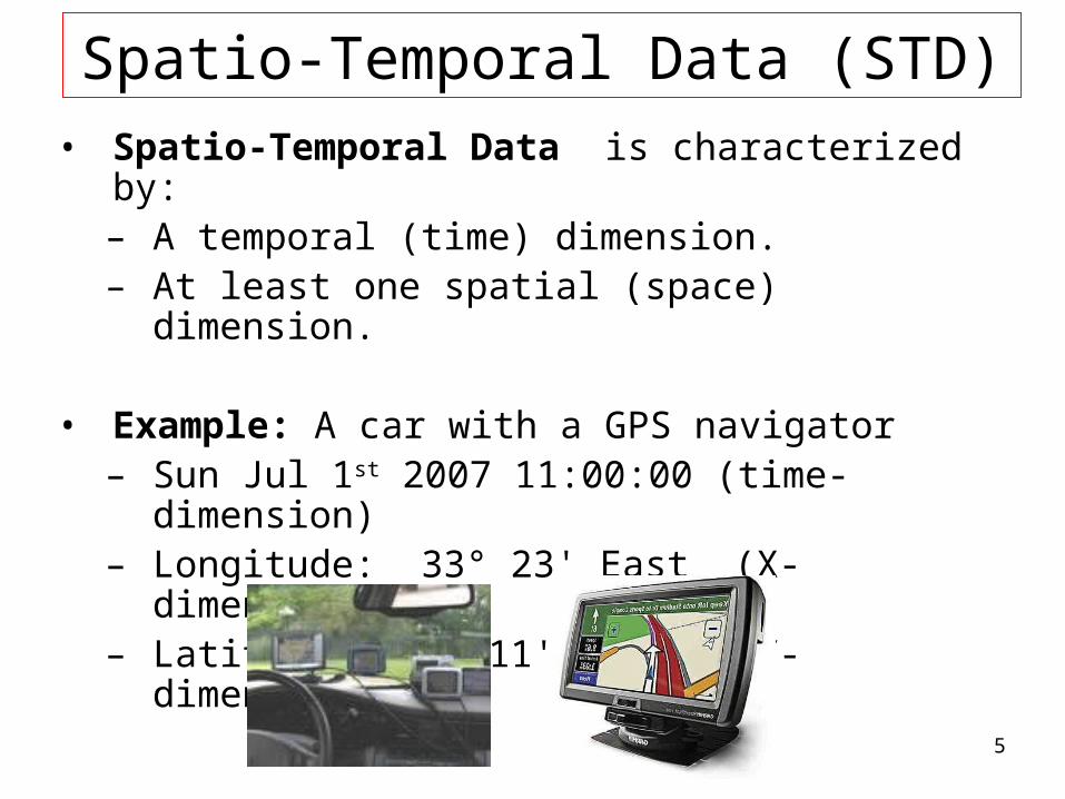
• Spatio-Temporal Data is characterized by:– A temporal (time) dimension.– At least one spatial (space) dimension.

• Example: A car with a GPS navigator– Sun Jul 1st 2007 11:00:00 (time-dimension)– Longitude: 33° 23' East (X-dimension)– Latitude: 35° 11' North (Y-dimension)

6

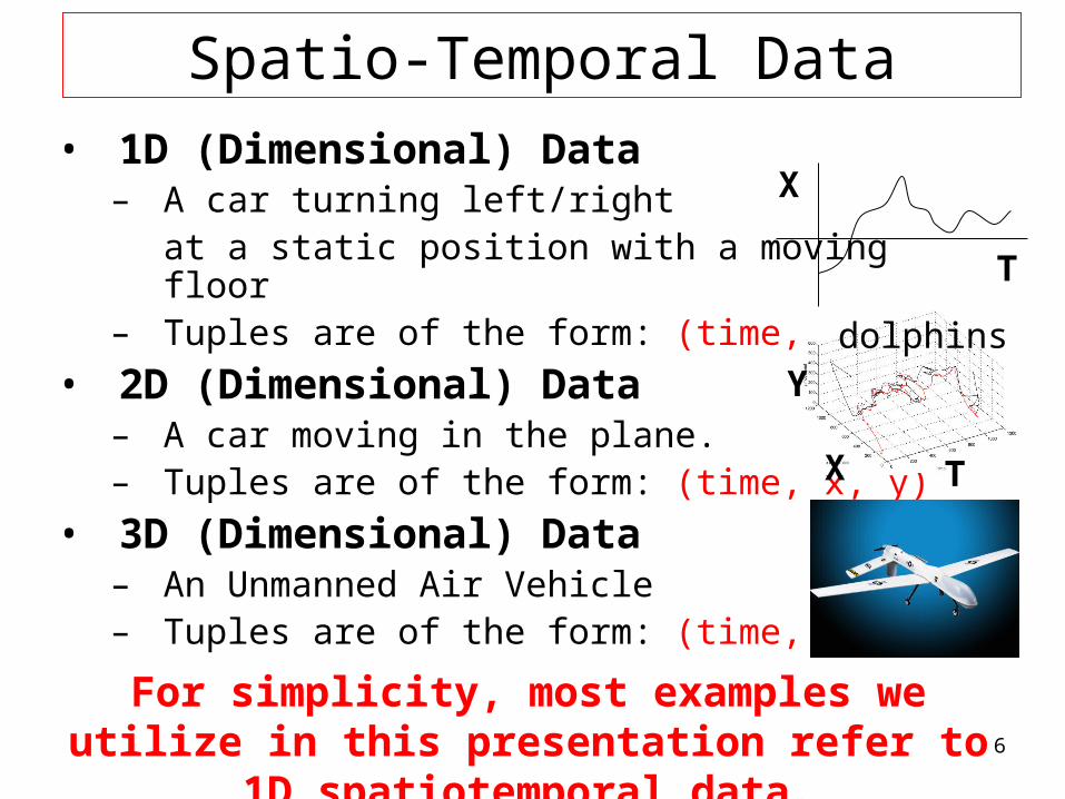
Spatio-Temporal Data

• 1D (Dimensional) Data– A car turning left/right

at a static position with a moving floor– Tuples are of the form: (time, x)

• 2D (Dimensional) Data– A car moving in the plane.– Tuples are of the form: (time, x, y)

• 3D (Dimensional) Data– An Unmanned Air Vehicle– Tuples are of the form: (time, x, y, z)

X

X

Y

T

For simplicity, most examples we utilize in this presentation refer to 1D spatiotemporal data.

T

dolphins

7

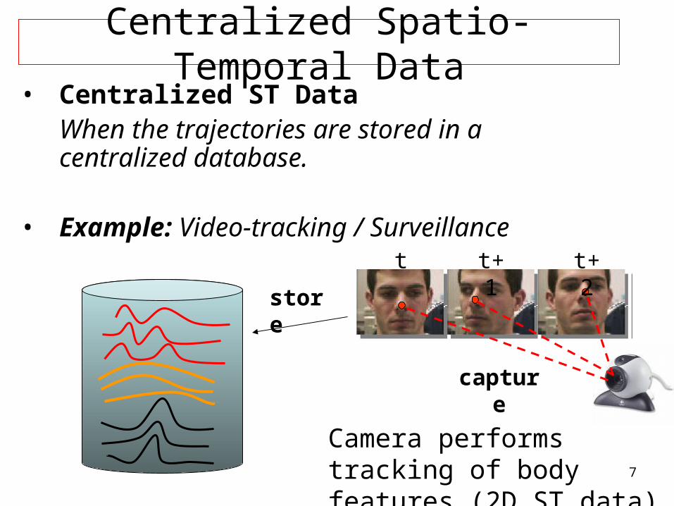
Centralized Spatio-Temporal Data• Centralized ST Data

When the trajectories are stored in a centralized database.

• Example: Video-tracking / Surveillance

Camera performs tracking of body features (2D ST data)

store

capture

t t+1 t+2

8

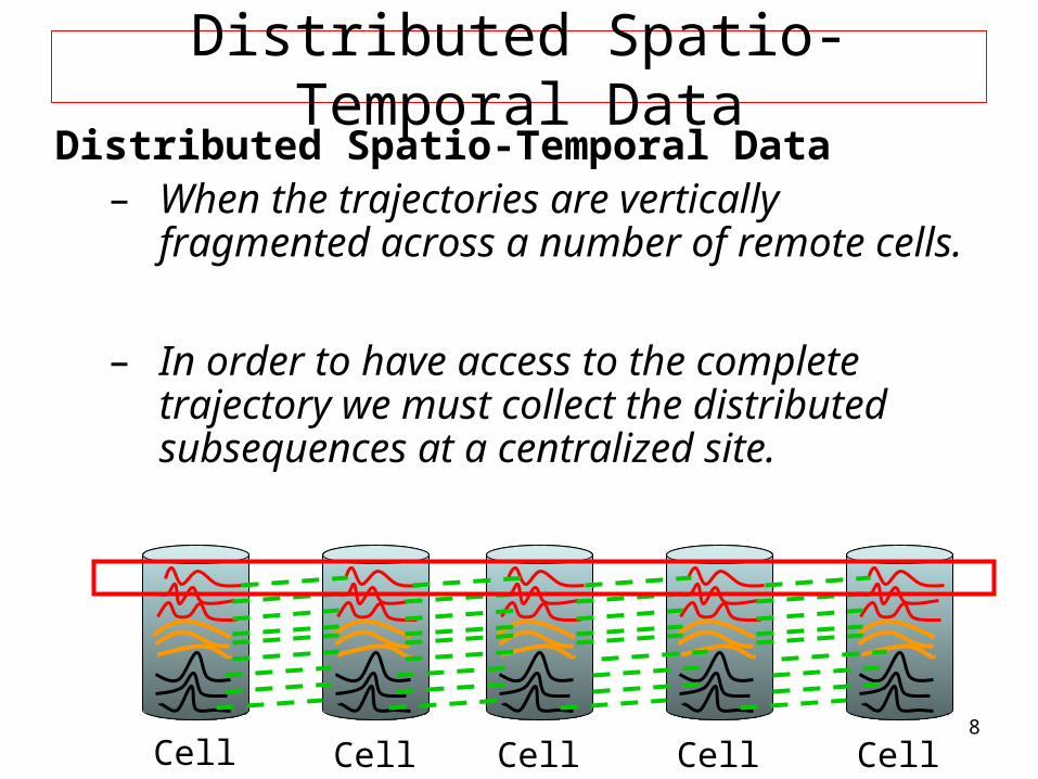
Distributed Spatio-Temporal DataDistributed Spatio-Temporal Data

– When the trajectories are vertically fragmented across a number of remote cells.

– In order to have access to the complete trajectory we must collect the distributed subsequences at a centralized site.

Cell 1 Cell 2 Cell 3 Cell 4 Cell 5

9

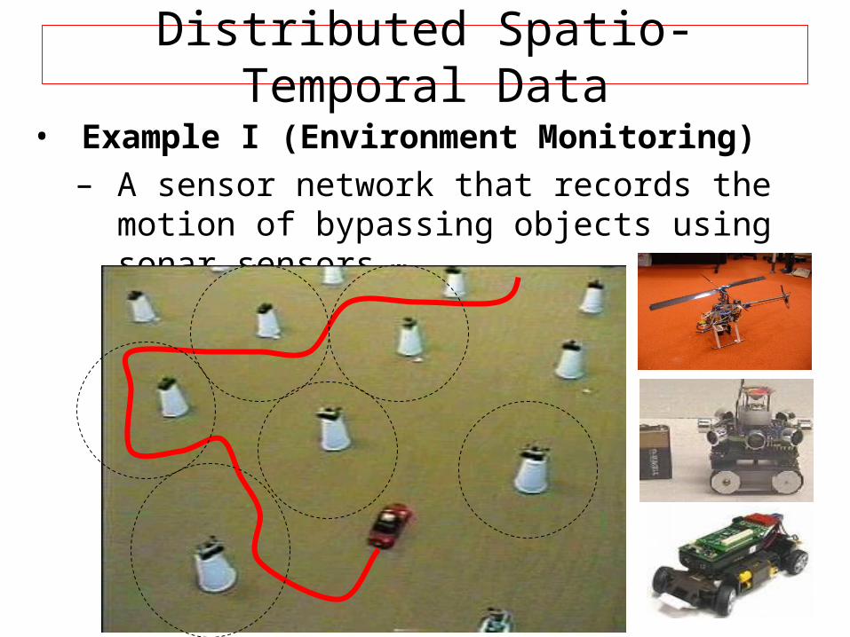
Distributed Spatio-Temporal Data

• Example I (Environment Monitoring)– A sensor network that records the motion of

bypassing objects using sonar sensors.

10

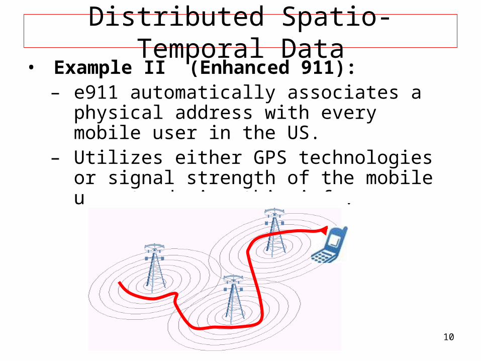
Distributed Spatio-Temporal Data• Example II (Enhanced 911):

– e911 automatically associates a physical address with every mobile user in the US.

– Utilizes either GPS technologies or signal strength of the mobile user to derive this info.

11

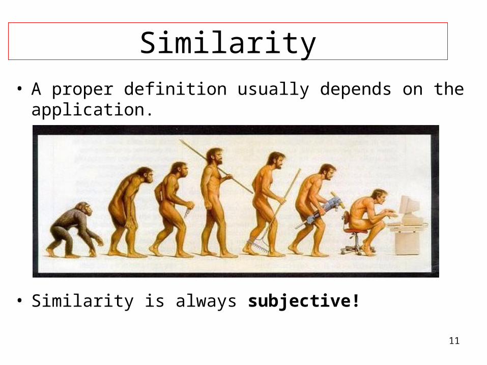
Similarity

• A proper definition usually depends on the application.

• Similarity is always subjective!

12

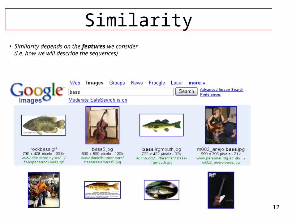
Similarity• Similarity depends on the features we consider

(i.e. how we will describe the sequences)

13

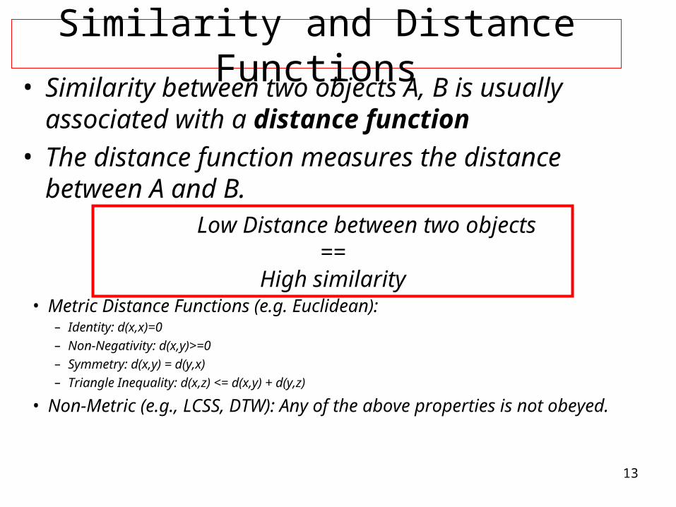
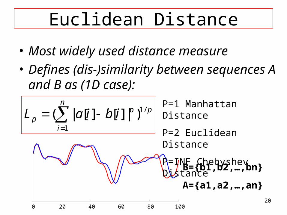
Similarity and Distance Functions• Similarity between two objects A, B is usually

associated with a distance function • The distance function measures the distance

between A and B.Low Distance between two objects

==High similarity

• Metric Distance Functions (e.g. Euclidean):– Identity: d(x,x)=0– Non-Negativity: d(x,y)>=0– Symmetry: d(x,y) = d(y,x)– Triangle Inequality: d(x,z) <= d(x,y) + d(y,z)

• Non-Metric (e.g., LCSS, DTW): Any of the above properties is not obeyed.

14

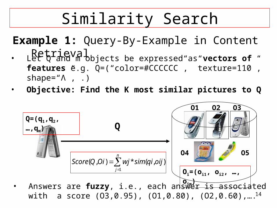
Similarity SearchExample 1: Query-By-Example in Content Retrieval

• Let Q and m objects be expressed as vectors of features e.g. Q=(“color=#CCCCCC”, ”texture=110”, shape=“Λ”, .)

• Objective: Find the K most similar pictures to Q

Q

O1 O2 O3

Q=(q1,q2,…,qm)

Oi=(oi1, oi2, …, oim)

O4 O5

• Answers are fuzzy, i.e., each answer is associated with a score (O3,0.95), (O1,0.80), (O2,0.60),….

n

j

oijqisimwjOiQScore1

),(*),(

15

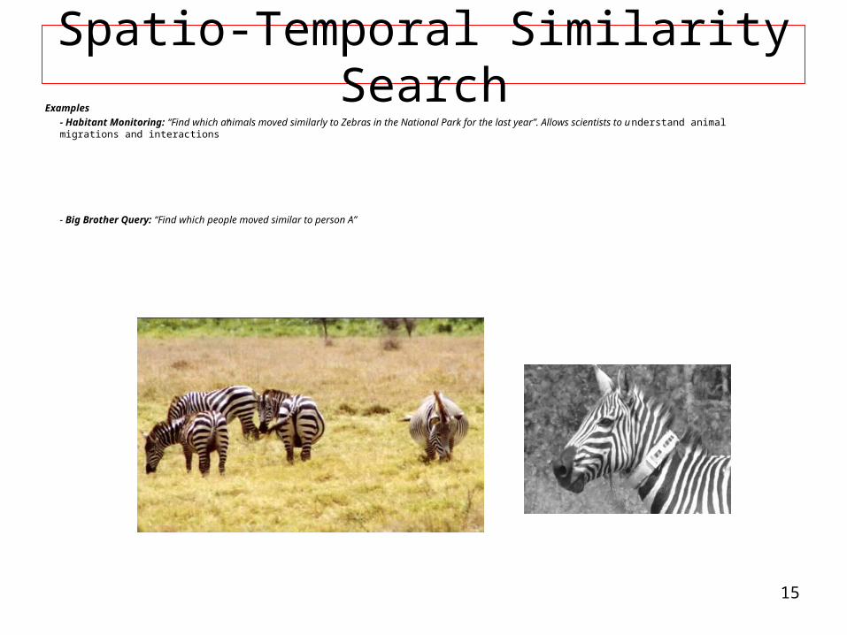
Spatio-Temporal Similarity SearchExamples

- Habitant Monitoring: “Find which animals moved similarly to Zebras in the National Park for the last year”. Allows scientists to understand animal migrations and interactions”

- Big Brother Query: “Find which people moved similar to person A”

16

Spatio-Temporal Similarity Search

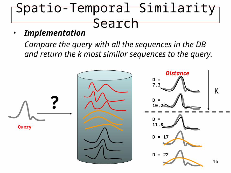
Query

D = 7.3

D = 10.2

D = 11.8

D = 17

D = 22

Distance

?

• Implementation

Compare the query with all the sequences in the DB and return the k most similar sequences to the query.

K

17

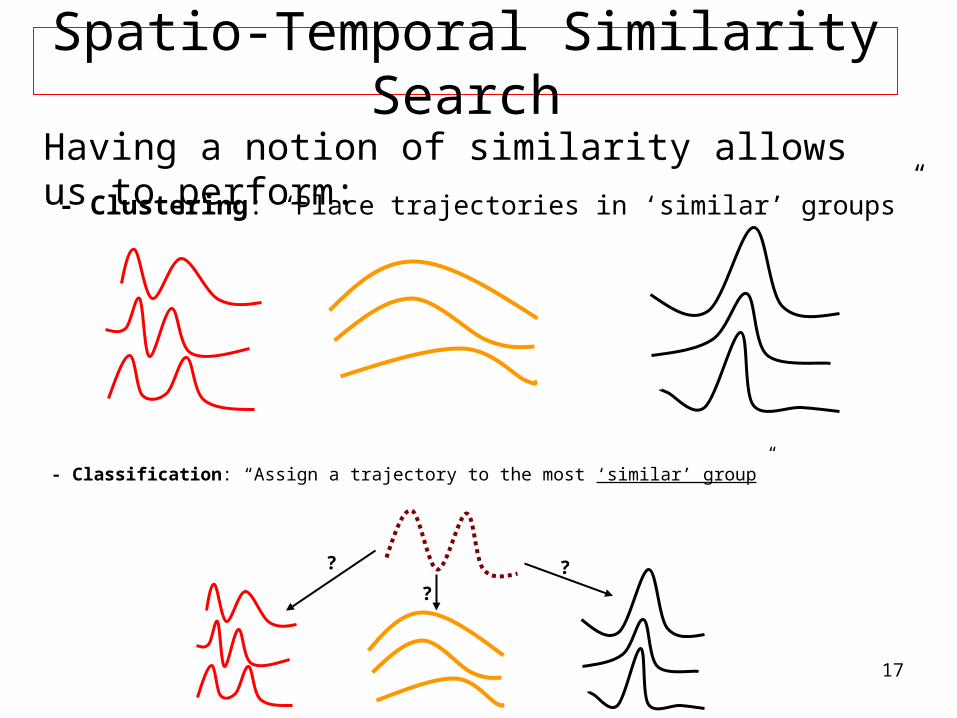
Spatio-Temporal Similarity Search

- Clustering: “Place trajectories in ‘similar’ groups”

- Classification: “Assign a trajectory to the most ‘similar’ group”

?

?

?

Having a notion of similarity allows us to perform:

18

Presentation Outline Definitions and Context Overview of Trajectory Similarity Measures

• Euclidean Matching• DTW Matching• LCSS Matching• Upper Bounding LCSS Matching

Distributed Spatio-Temporal Similarity Search• The UB-K Algorithm• The UBLB-K Algorithm• Experimentation

Distributed Top-K Algorithms • Definitions• The TJA Algorithm

Conclusions

19

Trajectory Similarity MeasuresA. Euclidean Matching

The trajectories are matched 1:1

B. Dynamic Time Warping MatchingCopes with out-of-phase matches (using a warping windows)

Longest Common SubSequence MatchingCopes with out-of-phase matches and outliers (it ignores them)

20

Euclidean Distance

n

i

ppp ibiaL

1

/1)|][][|(

0 20 40 60 80 100

• Most widely used distance measure

• Defines (dis-)similarity between sequences A and B as (1D case):

A={a1,a2,…,an}

B={b1,b2,…,bn}

P=1 Manhattan Distance

P=2 Euclidean Distance

P=INF Chebyshev Distance

21

Euclidean Distance• Euclidean vs. Manhattan distance:

- Euclidean Distance (using Pythagoras theorem) is 6 x √2 = 8.48 points): Diagonal Green line

- Manhattan (city-block) Distance (12 points): Red, Blue, and Yellow lines

0 1 2 3 4 5 6

0 1 2 3 4 56 a1

b1

2-Dimensional Scenario

22

Disadvantages of Lp-norms• Disadvantage 1: Not flexible to out-of-phase matching (i.e., temporal

distortions)– e.g., Compare the following 1-dim sequences:

A={1112234567}

B={1112223456}

Distance = 9– Green Lines indicate successful matching, while red dots indicate an increase in

distance.

• Disadvantage 2: Not flexible to outliers (spatial distortions).A={1111191111}

B={1111101111}

Distance = 9

Many studies show that the Euclidean Distance Error rate might be as high as ~30%!

23

Dynamic Time-WarpingFlexible matching in time: Used in speech recognition for matching words spoken at different speeds (in voice recognition systems)

----Mat-lab--------------------------

Same idea can work equally well for generic spatio-temporal data…

Sound signals

---Maat--llaabb-------------------

24

Euclidean distanceA1 = [1, 1, 2, 2] d = 1d = 1A2 = [1, 2, 2, 2]

Euclidean distanceA1 = [1, 1, 2, 2] d = 1d = 1A2 = [1, 2, 2, 2]

Dynamic Time-WarpingHow does it work?

The intuition is that we span the matching of an element X by several positions after X.

DTW distanceA1 = [1, 1, 2, 2] d = 0d = 0A2 = [1, 2, 2, 2]

DTW distanceA1 = [1, 1, 2, 2] d = 0d = 0A2 = [1, 2, 2, 2]

Euclidean: One-to-one alignment

DTW: One-to-many alignment

25

Dynamic Time-Warping

A

BRecursive DefinitionL[i,j] = LpNorm(Ai,Bj) + min{ L(i-1, j-1),

L(i-1, j ), L(i, j-1) }

Recursive DefinitionL[i,j] = LpNorm(Ai,Bj) + min{ L(i-1, j-1),

L(i-1, j ), L(i, j-1) }

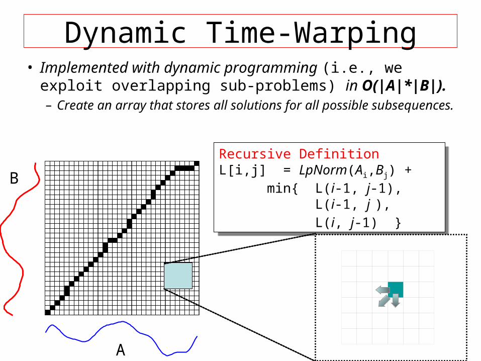
• Implemented with dynamic programming (i.e., we exploit overlapping sub-problems) in O(|A|*|B|). – Create an array that stores all solutions for all possible

subsequences.

26

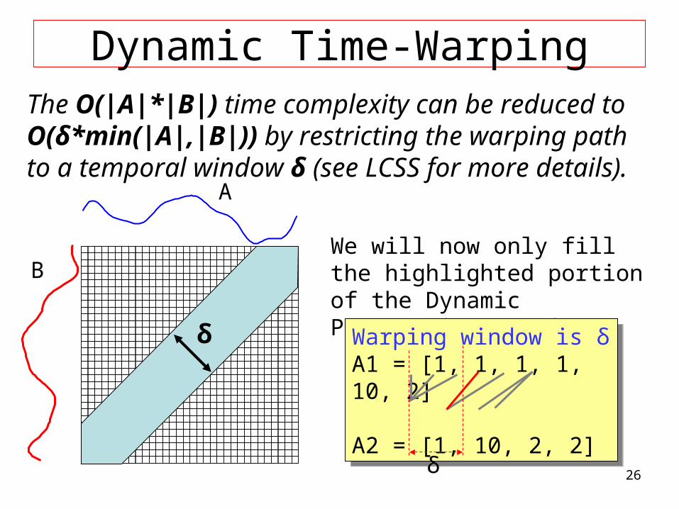
Dynamic Time-WarpingThe O(|A|*|B|) time complexity can be reduced to O(δ*min(|A|,|B|)) by restricting the warping path to a temporal window δ (see LCSS for more details).

A

BWe will now only fill the highlighted portion of the Dynamic Programming matrix

Warping window is δA1 = [1, 1, 1, 1, 10, 2]

A2 = [1, 10, 2, 2]

Warping window is δA1 = [1, 1, 1, 1, 10, 2]

A2 = [1, 10, 2, 2]

δ

δ

27

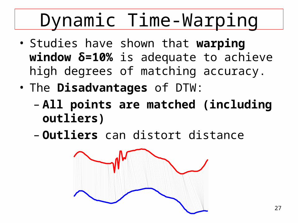
Dynamic Time-Warping• Studies have shown that warping window

δ=10% is adequate to achieve high degrees of matching accuracy.

• The Disadvantages of DTW:– All points are matched (including outliers)– Outliers can distort distance

28

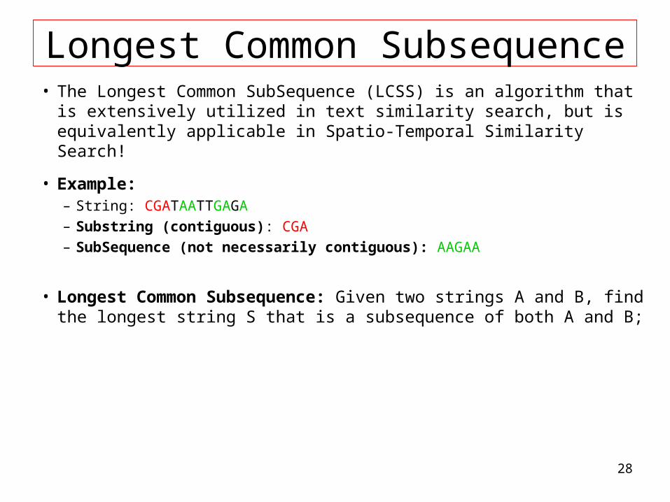
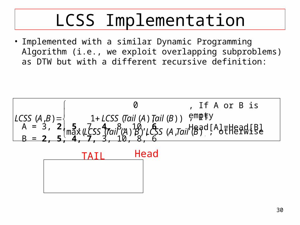
Longest Common Subsequence• The Longest Common SubSequence (LCSS) is an algorithm that

is extensively utilized in text similarity search, but is equivalently applicable in Spatio-Temporal Similarity Search!

• Example:– String: CGATAATTGAGA – Substring (contiguous): CGA– SubSequence (not necessarily contiguous): AAGAA

• Longest Common Subsequence: Given two strings A and B, find the longest string S that is a subsequence of both A and B;

29

Longest Common Subsequence• Find the LCSS of the following 1D-trajectory

A = 3, 2, 5, 7, 4, 8, 10, 7

B = 2, 5, 4, 7, 3, 10, 8, 6

LCSS = 2, 5, 4, 7• The value of LCSS is unbounded: it depends on the length of the

compared sequences.• To normalize it in order to support sequences of variable length we can

define the LCSS distance:• LCSS Distance between two trajectories

dist(A, B) = 1 – LCSS(A,B)/min(|A|,|B|)

e.g. in our example dist (A,B) = 1 – 4/8 = 0.5

30

LCSS Implementation• Implemented with a similar Dynamic Programming Algorithm

(i.e., we exploit overlapping subproblems) as DTW but with a different recursive definition:

A = 3, 2, 5, 7, 4, 8, 10, 6

B = 2, 5, 4, 7, 3, 10, 8, 6

))(,(),),((max(

))(),((1

0

),(

BTailALCSSBATailLCSS

BTailATailLCSSBALCSS

, If A or B is empty

, If Head[A]=Head[B]

, otherwise

TAIL Head

31

LCSS ImplementationPhase 1: Construct DP Tableint A[] = {3,2,5,7,4,8,10,7};

int B[] = {2,5,4,7,3,10,8,6};

int L[n+1][m+1]; // DP Table

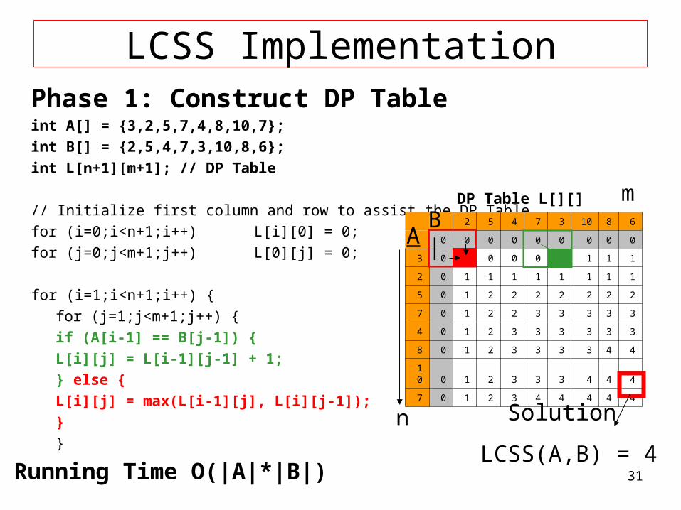
// Initialize first column and row to assist the DP Table

for (i=0;i<n+1;i++) L[i][0] = 0;

for (j=0;j<m+1;j++) L[0][j] = 0;

for (i=1;i<n+1;i++) {

for (j=1;j<m+1;j++) {

if (A[i-1] == B[j-1]) {

L[i][j] = L[i-1][j-1] + 1;

} else {

L[i][j] = max(L[i-1][j], L[i][j-1]);

}

}

DP Table L[][]

    2 5 4 7 3 10 8 6

  0 0 0 0 0 0 0 0 0

3 0 0 0 0 0 1 1 1 1

2 0 1 1 1 1 1 1 1 1

5 0 1 2 2 2 2 2 2 2

7 0 1 2 2 3 3 3 3 3

4 0 1 2 3 3 3 3 3 3

8 0 1 2 3 3 3 3 4 4

10 0 1 2 3 3 3 4 4 4

7 0 1 2 3 4 4 4 4 4

Running Time O(|A|*|B|)

Solution

LCSS(A,B) = 4

n

mB|

A

32

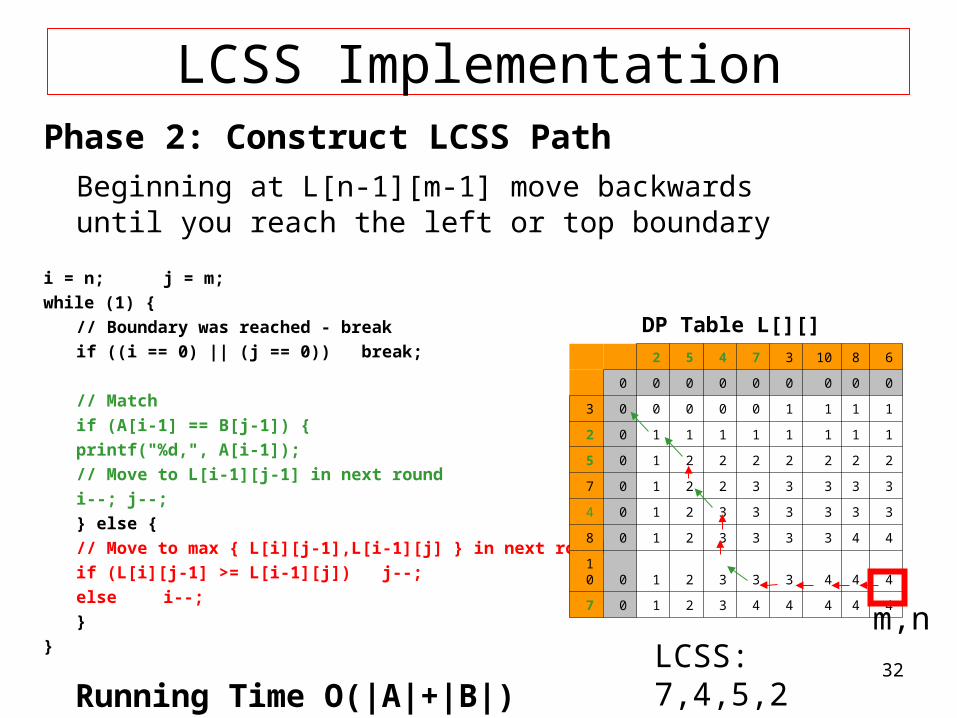
LCSS ImplementationPhase 2: Construct LCSS Path

Beginning at L[n-1][m-1] move backwards until you reach the left or top boundary

i = n; j = m;

while (1) {

// Boundary was reached - break

if ((i == 0) || (j == 0)) break;

// Match

if (A[i-1] == B[j-1]) {

printf("%d,", A[i-1]);

// Move to L[i-1][j-1] in next round

i--; j--;

} else {

// Move to max { L[i][j-1],L[i-1][j] } in next round

if (L[i][j-1] >= L[i-1][j]) j--;

else i--;

}

}

DP Table L[][]

    2 5 4 7 3 10 8 6

  0 0 0 0 0 0 0 0 0

3 0 0 0 0 0 1 1 1 1

2 0 1 1 1 1 1 1 1 1

5 0 1 2 2 2 2 2 2 2

7 0 1 2 2 3 3 3 3 3

4 0 1 2 3 3 3 3 3 3

8 0 1 2 3 3 3 3 4 4

10 0 1 2 3 3 3 4 4 4

7 0 1 2 3 4 4 4 4 4

Running Time O(|A|+|B|)LCSS: 7,4,5,2

m,n

33

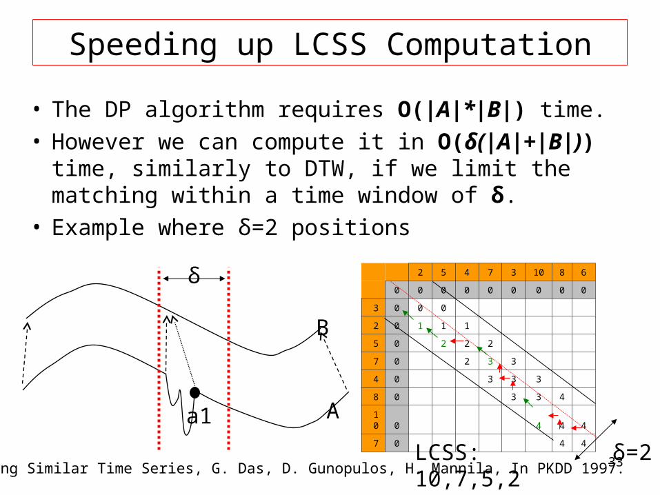
Speeding up LCSS Computation

• The DP algorithm requires O(|A|*|B|) time. • However we can compute it in O(δ(|A|+|B|))

time, similarly to DTW, if we limit the matching within a time window of δ.

• Example where δ=2 positions

* Finding Similar Time Series, G. Das, D. Gunopulos, H. Mannila, In PKDD 1997.

δ

A

    2 5 4 7 3 10 8 6

  0 0 0 0 0 0 0 0 0

3 0 0 0            

2 0 1 1 1          

5 0   2 2 2        

7 0     2 3 3      

4 0       3 3 3    

8 0         3 3 4  

10 0           4 4 4

7 0             4 4

δ=2LCSS: 10,7,5,2

B

a1

34

LCSS 2D Computation

• The LCSS concept can easily be extended to support 2D (or higher dimensional) spatio-temporal data.

• The following is an adaptation to the 2D case, where the computation is limited in time (by window δ) and space (by window ε)

1 2 1 2

0, if or is empty

1 ( ( ), ( )),

( , ) if - and

( ( ( ), ), ( , ( )),

otherwis

i i

A B

LCSS Tail A Tail B

LCSS A B a b i i

max LCSS Tail A B LCSS A Tail B

e

35

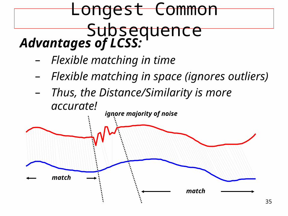
Longest Common Subsequence

ignore majority of noise

match

match

Advantages of LCSS:– Flexible matching in time– Flexible matching in space (ignores outliers)– Thus, the Distance/Similarity is more

accurate!

36

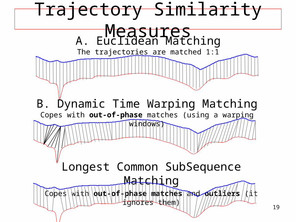
Summary of Distance Measures

Method Complexity* Elastic Matching

(out-of-phase)

1:1 Matching Noise Robustness

(outliers)

Euclidean O(n)

DTW O(n*δ)

LCSS O(n*δ) * Assuming that trajectories have the same length

Any disadvantage with LCSS?

37

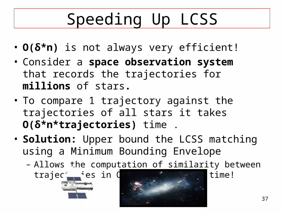
Speeding Up LCSS

• O(δ*n) is not always very efficient!• Consider a space observation system that

records the trajectories for millions of stars. • To compare 1 trajectory against the trajectories

of all stars it takes O(δ*n*trajectories) time .• Solution: Upper bound the LCSS matching

using a Minimum Bounding Envelope– Allows the computation of similarity between

trajectories in O(n*trajectories) time!

38

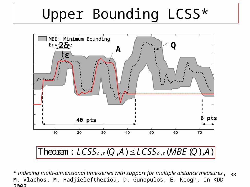
Upper Bounding LCSS*

, ,Theorem: ( , ) ( ( ), )LCSS Q A LCSS MBE Q A

* Indexing multi-dimensional time-series with support for multiple distance measures,M. Vlachos, M. Hadjieleftheriou, D. Gunopulos, E. Keogh, In KDD 2003.

QAε

2δ

40 pts 6 pts

ΜΒΕ: Minimum Bounding Envelope

39

Presentation Outline Definitions and Context Overview of Trajectory Similarity Measures

• Euclidean Matching • DTW Matching• LCSS Matching • Upper Bounding LCSS Matching

Distributed Spatio-Temporal Similarity Search• Definitions• The UB-K and UBLB-K Algorithms• Experimentation

Distributed Top-K Algorithms • Definitions• The TJA Algorithm

Conclusions

40

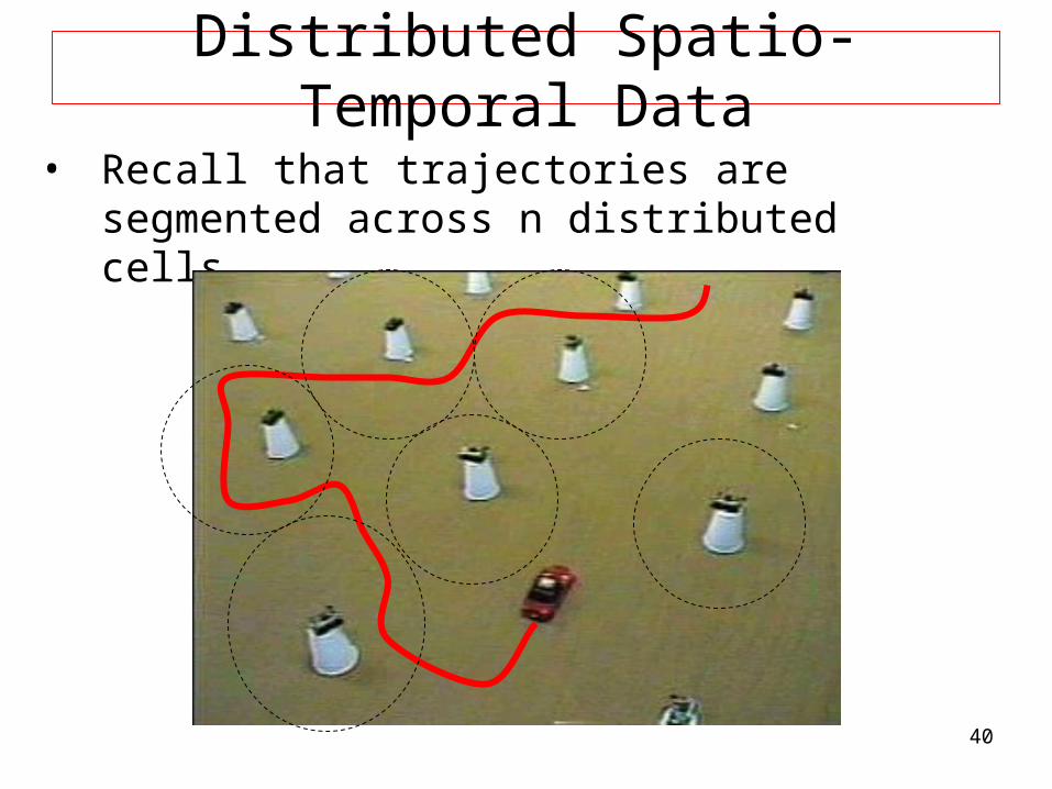
Distributed Spatio-Temporal Data

• Recall that trajectories are segmented across n distributed cells.

41

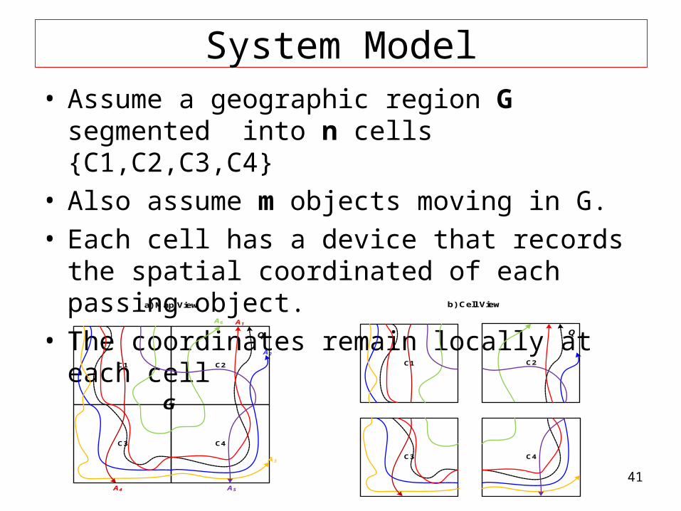
System Model• Assume a geographic region G segmented into

n cells {C1,C2,C3,C4}• Also assume m objects moving in G.• Each cell has a device that records the spatial

coordinated of each passing object.• The coordinates remain locally at each cell

C1 C2

C3 C4

A2

A1

Q

a) Map View b) Cell View

G

A3

A4 A5

A6

C1 C2

Q

C3 C4

42

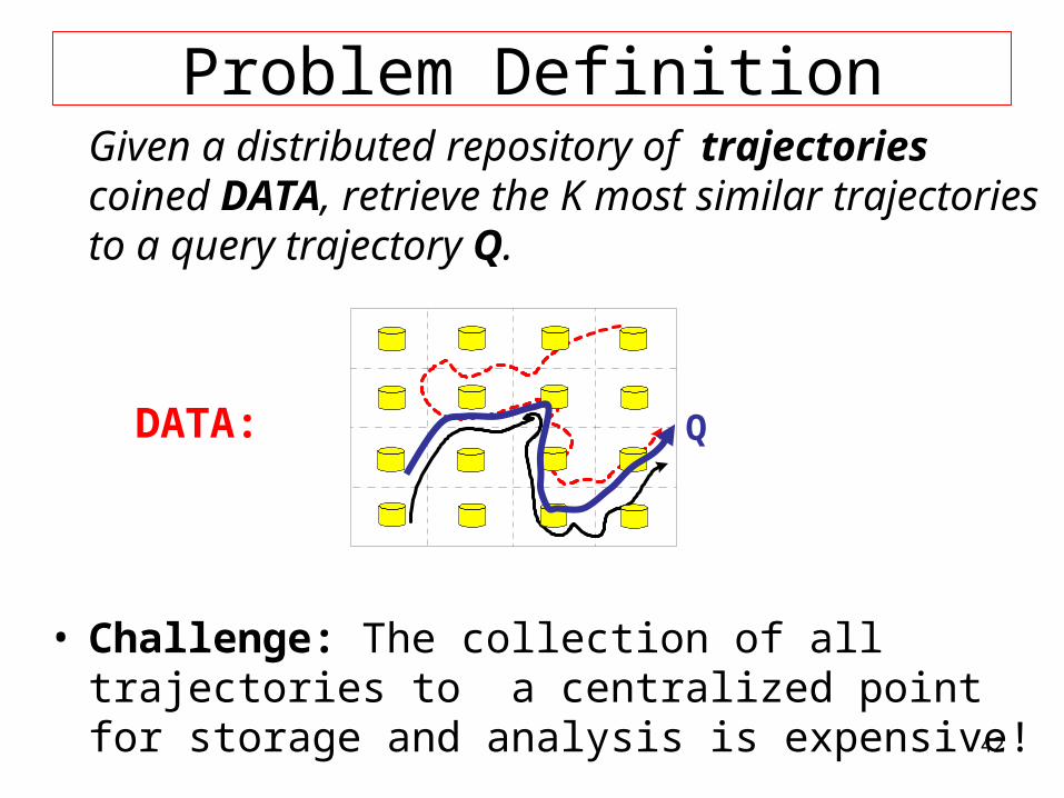
Problem DefinitionGiven a distributed repository of trajectories coined DΑΤΑ, retrieve the K most similar trajectories to a query trajectory Q.

• Challenge: The collection of all trajectories to a centralized point for storage and analysis is expensive!

QDATA:

43

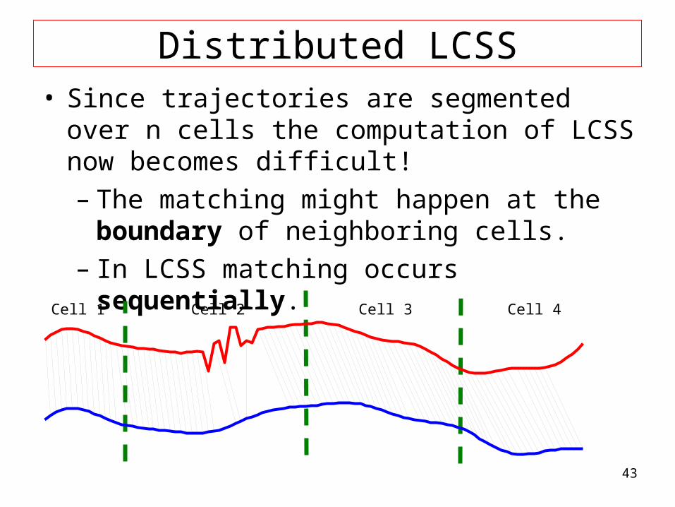
Distributed LCSS• Since trajectories are segmented over n cells the

computation of LCSS now becomes difficult!– The matching might happen at the boundary

of neighboring cells. – In LCSS matching occurs sequentially.

Cell 1 Cell 2 Cell 3 Cell 4

44

Distributed LCSS

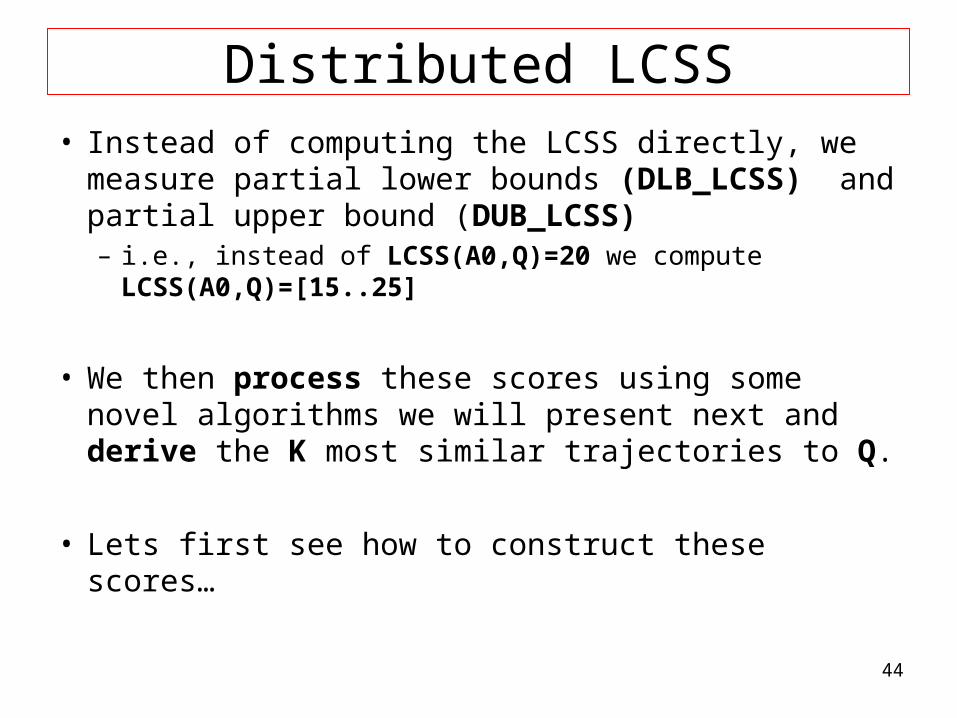
• Instead of computing the LCSS directly, we measure partial lower bounds (DLB_LCSS) and partial upper bound (DUB_LCSS) – i.e., instead of LCSS(A0,Q)=20 we compute

LCSS(A0,Q)=[15..25]

• We then process these scores using some novel algorithms we will present next and derive the K most similar trajectories to Q.

• Lets first see how to construct these scores…

45

QAε

2δ

40 pts 6 pts

ΜΒΕ: Minimum Bounding Envelope

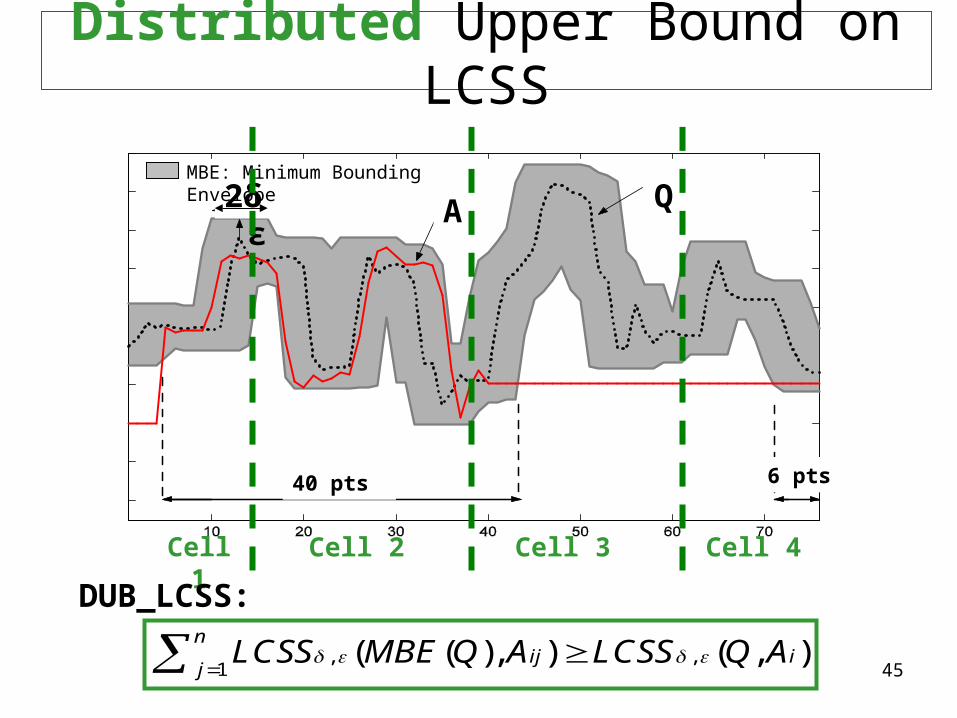
Distributed Upper Bound on LCSS

Cell 1 Cell 2 Cell 3 Cell 4

, ,1

( ( ), ) ( , )n

ij ijLCSS MBE Q A LCSS Q A

DUB_LCSS:

46

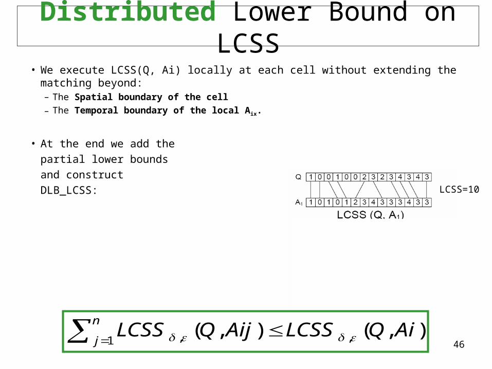
Distributed Lower Bound on LCSS• We execute LCSS(Q, Ai) locally at each cell without extending the matching

beyond:– The Spatial boundary of the cell

– The Temporal boundary of the local Aix.

• At the end we add the

partial lower bounds

and construct

DLB_LCSS:

n

jAiQLCSSAijQLCSS

1 ,, ),(),(

Cell1 Cell2

LCSS=10

LCSS=4+5=9

47

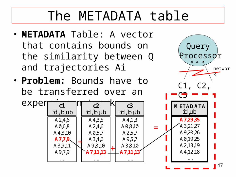
The METADATA table• METADATA Table: A vector that

contains bounds on the similarity between Q and trajectories Ai

• Problem: Bounds have to be transferred over an expensive network

Query Processor

C1, C2, C3

A7,29,35A3,21,27A9,20,26A0,19,25A2,13,19A4,12,18

....

A2,4,6A0,6,8A4,8,10A7,7,9A3,9,11A9,7,9

....

A4,3,5A2,4,6A0,5,7A3,4,6A9,8,10A7,11,13

....

A4,1,3A0,8,10A2,5,7A9,5,7A3,8,10A7,11,13

....

id,lb,ubc3

id,lb,ubc2

id,lb,ubc1

id,ubMETADATA

++

=

network

48

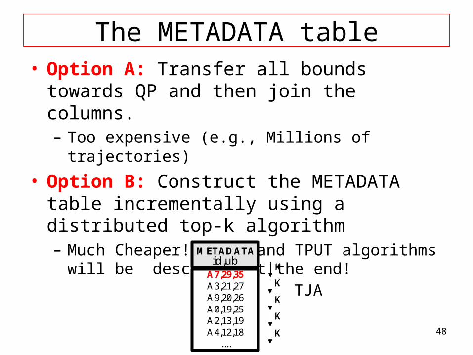
The METADATA table• Option A: Transfer all bounds towards QP and

then join the columns.– Too expensive (e.g., Millions of trajectories)

• Option B: Construct the METADATA table incrementally using a distributed top-k algorithm – Much Cheaper! - TJA and TPUT algorithms will be

described at the end!

K

TJAK

K

K

K

K

K

K

K

K

A7,29,35A3,21,27A9,20,26A0,19,25A2,13,19A4,12,18

....

id,ubMETADATA

49

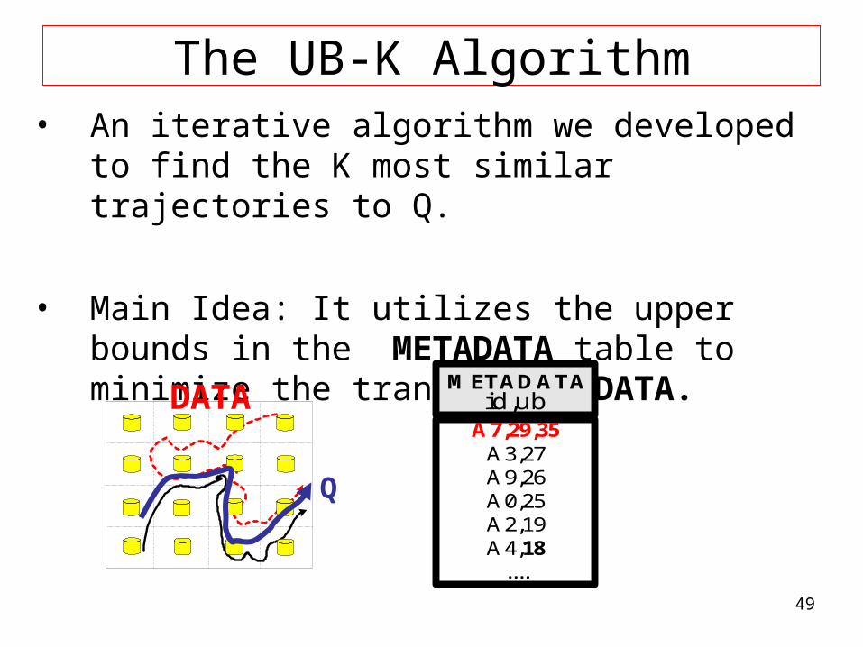
The UB-K Algorithm• An iterative algorithm we developed to find the K

most similar trajectories to Q.

• Main Idea: It utilizes the upper bounds in the METADATA table to minimize the transfer of DATA.

Q

DATAA7,29,35

A3,27A9,26A0,25A2,19A4,18

....

id,ubMETADATA

50

UB-K Execution

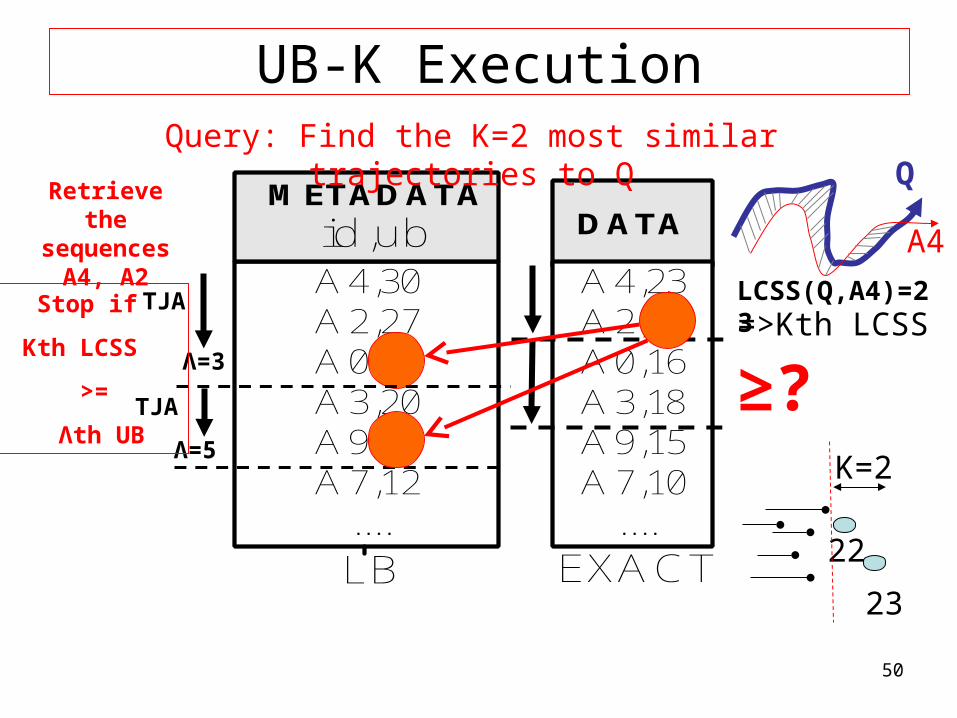
A4,30A2,27A0,25A3,20A9,18A7,12....

id,lbid,ub

A4,23A2,22A0,16A3,18A9,15A7,10....

DATAMETADATA

LB EXACT

Query: Find the K=2 most similar trajectories to Q

Λ=5

TJA ≥?Λ=3

TJA

Q

A4

LCSS(Q,A4)=23

Retrieve the sequences A4,

A2

Stop if

Kth LCSS

>=

Λth UB

=>Kth LCSS

23

22

K=2

51

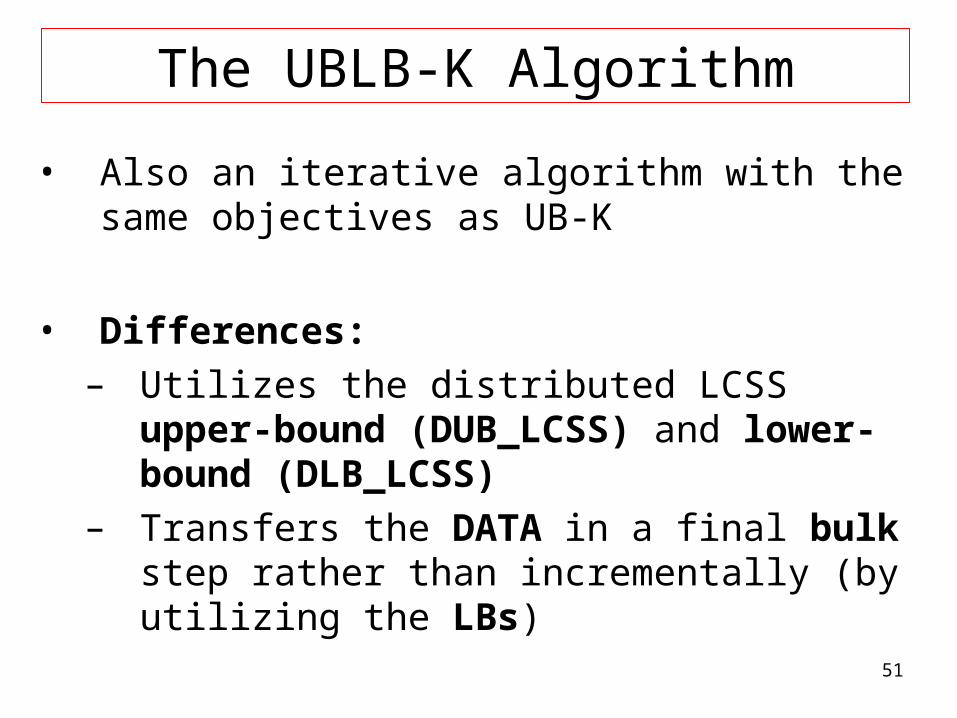
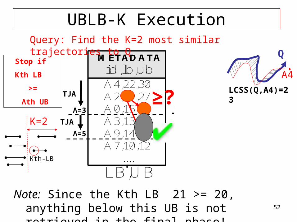
The UBLB-K Algorithm

• Also an iterative algorithm with the same objectives as UB-K

• Differences: – Utilizes the distributed LCSS upper-bound

(DUB_LCSS) and lower-bound (DLB_LCSS)– Transfers the DATA in a final bulk step rather

than incrementally (by utilizing the LBs)

52

A4,22,30A2,21,27A0,15,25A3,13,20A9,14,18A7,10,12

....

id,lbid,lb,ub

METADATA

Exact Score

LB,UB

A4,23A2,22A0,16A3,18A9,15A7,10....

DATA

EXACT

Note: Since the Kth LB 21 >= 20, anything below this UB is not retrieved in the final phase!

Λ=3

TJA ≥?

UBLB-K ExecutionQuery: Find the K=2 most similar trajectories to Q

TJA

Λ=5

≥?

Stop if

Kth LB

>=

Λth UB

K=2

Kth-LB

Q

A4

LCSS(Q,A4)=23

53

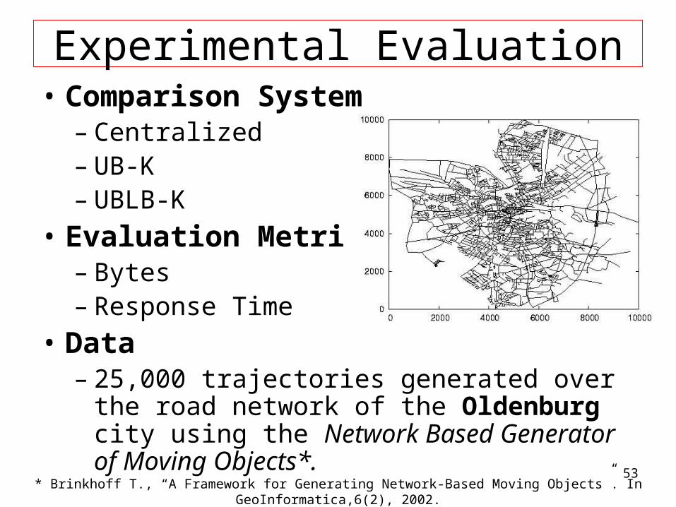
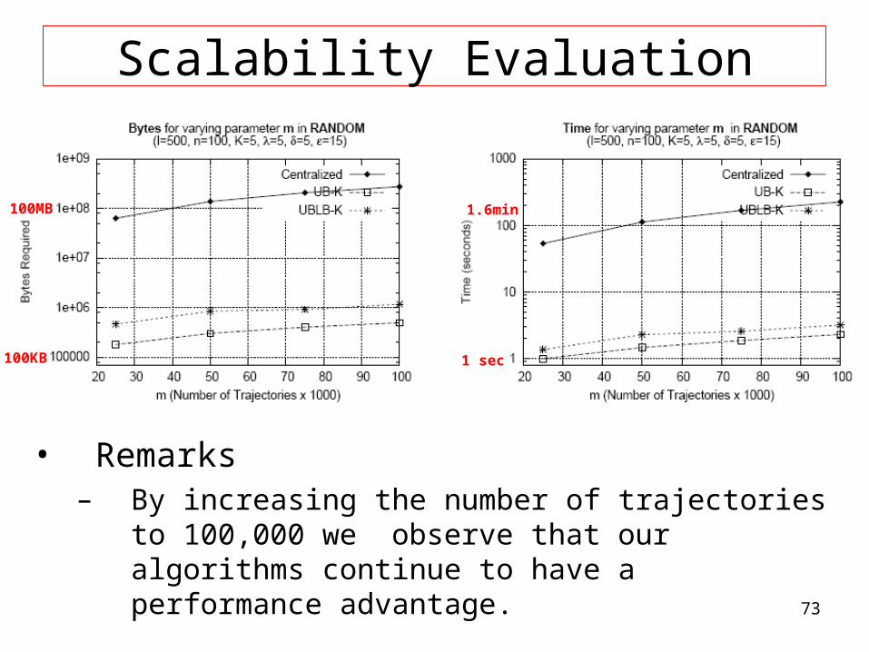
Experimental Evaluation• Comparison System

– Centralized– UB-K– UBLB-K

• Evaluation Metrics– Bytes– Response Time

• Data– 25,000 trajectories generated over the road

network of the Oldenburg city using the Network Based Generator of Moving Objects*.

* Brinkhoff T., “A Framework for Generating Network-Based Moving Objects”. In GeoInformatica,6(2), 2002.

54

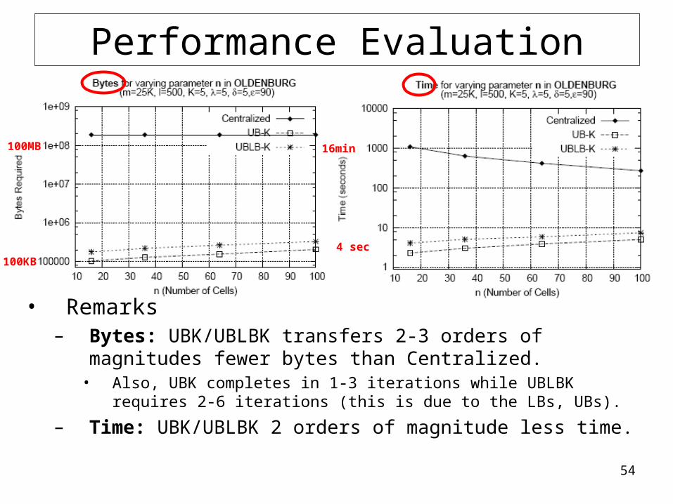
Performance Evaluation

• Remarks– Bytes: UBK/UBLBK transfers 2-3 orders of

magnitudes fewer bytes than Centralized.• Also, UBK completes in 1-3 iterations while UBLBK requires

2-6 iterations (this is due to the LBs, UBs).

– Time: UBK/UBLBK 2 orders of magnitude less time.

100ΜΒ

100ΚΒ

16min

4 sec

55

Presentation Outline Definitions and Context Overview of Trajectory Similarity Measures

• Euclidean Matching • DTW Matching• LCSS Matching • Upper Bounding LCSS Matching

Distributed Spatio-Temporal Similarity Search• Definitions• The UB-K and UBLB-K Algorithms• Experimentation

Distributed Top-K Algorithms • Definitions• The TJA Algorithm

Conclusions

56

DefinitionsTop-K Query (Q)Given a database D of n objects, a scoring function (according to which we rank the objects in D) and the number of expected answers K, a Top-K query Q returns the K objects with the highest score (rank) in D.

Objective:Trade # of answers with the query execution cost, i.e.,• Return less results (K<<n objects)• …but minimize the cost that is associated with

the retrieval of the answer set (i.e., disk I/Os, network I/Os, CPU etc)

57

Definitions

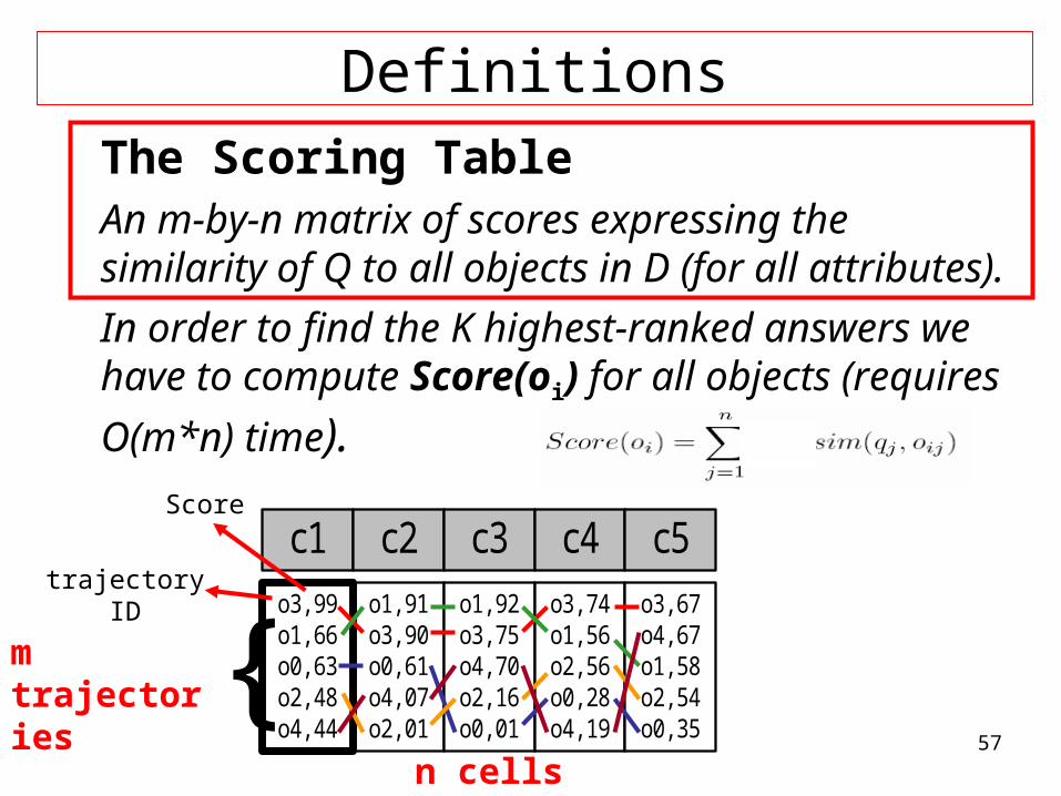
The Scoring TableAn m-by-n matrix of scores expressing the similarity of Q to all objects in D (for all attributes).

In order to find the K highest-ranked answers we have to compute Score(oi) for all objects

(requires O(m*n) time).

c1 c2 c3 c4 c5o1, 91o3, 90o0, 61o4, 07o2, 01

o1, 92o3, 75o4, 70o2, 16o0, 01

o3, 74o1, 56o2, 56o0, 28o4, 19

o3, 67o4, 67o1, 58o2, 54o0, 35

TOP-1

o3, 405o1, 363o4, 207o0, 188o2, 175

o3,405o3, 99o1, 66o0, 63o2, 48o4, 44

{m trajectories

n cells

Score

TOTAL SCORE

trajectoryID

58

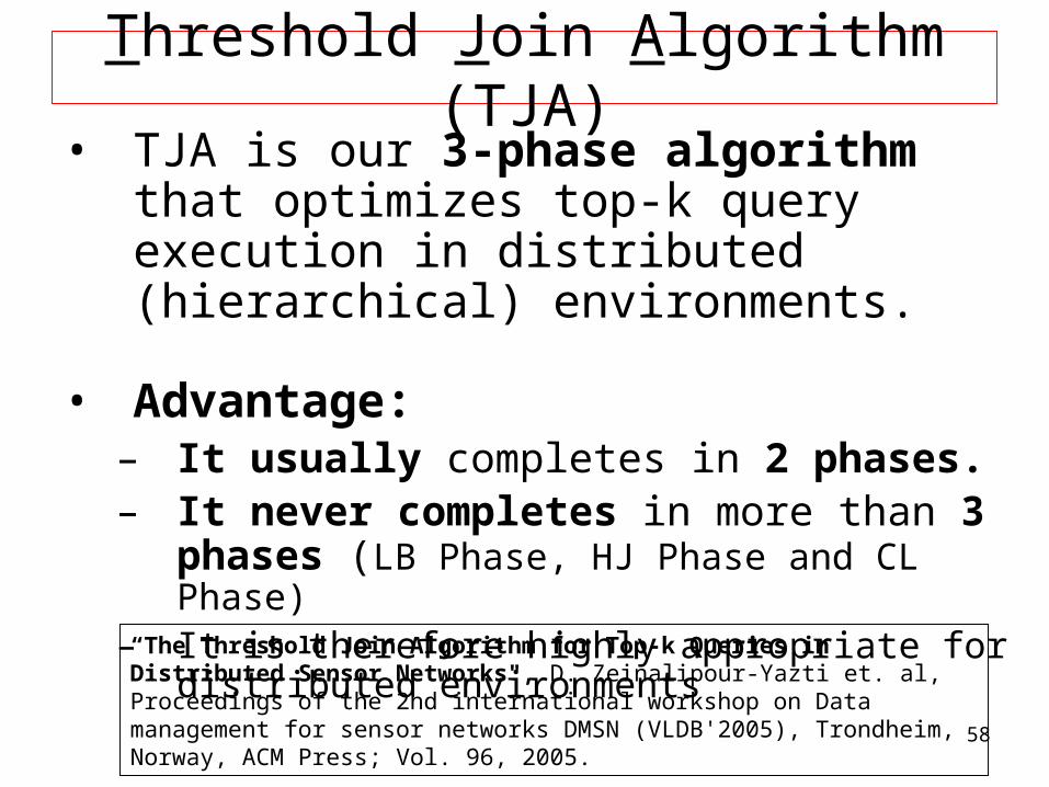
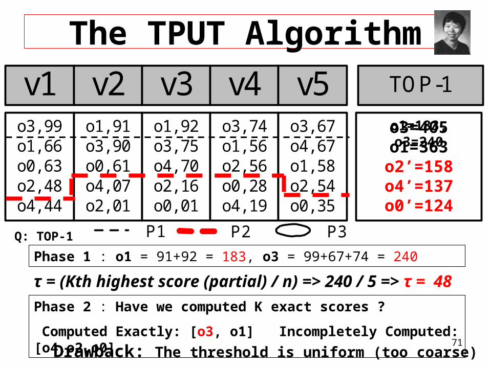
Threshold Join Algorithm (TJA)• TJA is our 3-phase algorithm that

optimizes top-k query execution in distributed (hierarchical) environments.

• Advantage:– It usually completes in 2 phases.– It never completes in more than 3 phases

(LB Phase, HJ Phase and CL Phase)– It is therefore highly appropriate for distributed

environments

“The Threshold Join Algorithm for Top-k Queries in Distributed Sensor Networks", D. Zeinalipour-Yazti et. al, Proceedings of the 2nd international workshop on Data management for sensor networks DMSN (VLDB'2005), Trondheim, Norway, ACM Press; Vol. 96, 2005.

59

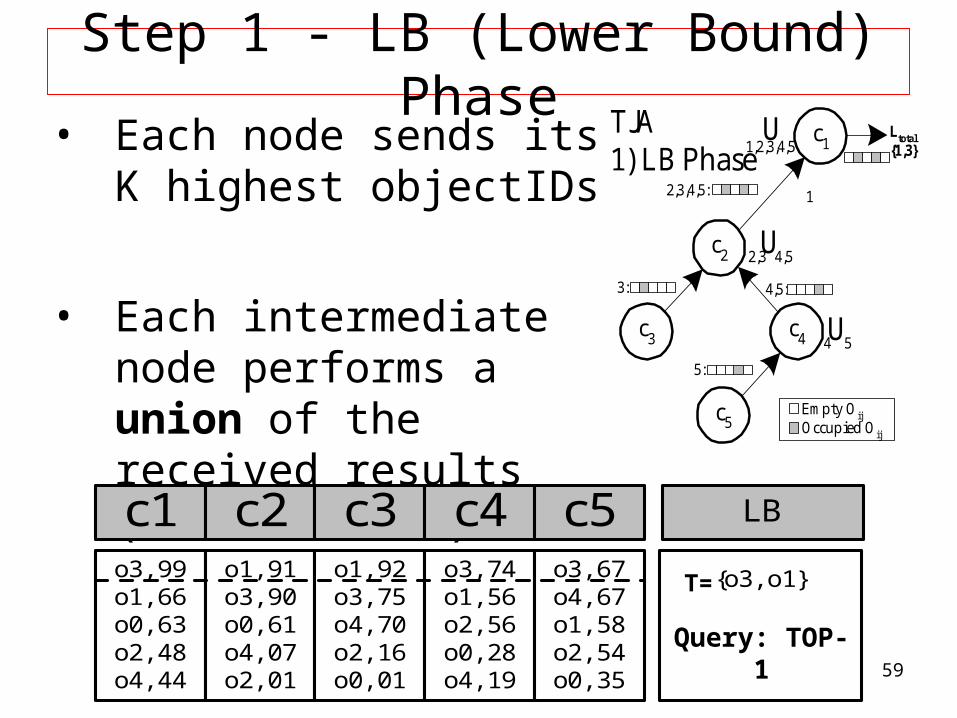
Step 1 - LB (Lower Bound) Phase• Each node sends its K

highest objectIDs

• Each intermediate node performs a union of the received results (defined as τ):

c1

c3

c2

c4

c5

5:

3:

2,3,4,5:

TJA1) LB Phase

4,5:

4U5

2,3U4,5

U

1

1,2,3,4,5Ltotal{1,3}

Occupied Oij

Empty Oij

c1 c2 c3 c4 c5o3, 99o1, 66o0, 63o2, 48o4, 44

o1, 91o3, 90o0, 61o4, 07o2, 01

o1, 92o3, 75o4, 70o2, 16o0, 01

o3, 74o1, 56o2, 56o0, 28o4, 19

o3, 67o4, 67o1, 58o2, 54o0, 35

LB

{o3, o1}

Query: TOP-1

Τ=

60

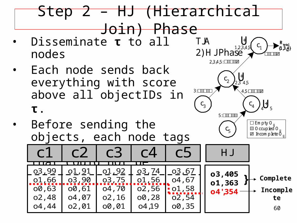
Step 2 – HJ (Hierarchical Join) Phase• Disseminate τ to all nodes • Each node sends back

everything with score above all objectIDs in τ.

• Before sending the objects, each node tags as incomplete, scores that could not be computed exactly (upper bound)

TJA2) HJ Phase

c1

c3

c2

c4

c5

5:

3:

2,3,4,5:

4,5:

4 5

2,3 4,5

1,2,3,4,5Rtotal{1,3,4}

Occupied Oij

Empty Oij

Incomplete Oij

U+

U+

U+

o3, 405o1, 363o4',354

c1 c2 c3 c4 c5o3, 99o1, 66o0, 63o2, 48o4, 44

o1, 91o3, 90o0, 61o4, 07o2, 01

o1, 92o3, 75o4, 70o2, 16o0, 01

o3, 74o1, 56o2, 56o0, 28o4,19

o3, 67o4, 67o1, 58o2, 54o0, 35

HJ

} Complete

Incomplete

61

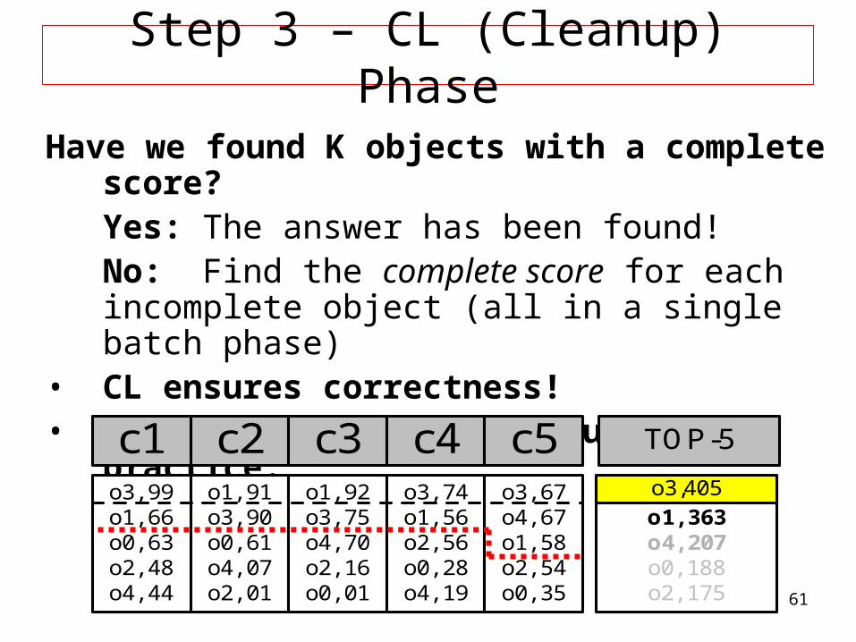
Step 3 – CL (Cleanup) Phase

Have we found K objects with a complete score?Yes: The answer has been found!No: Find the complete score for each incomplete object (all in a single batch phase)

• CL ensures correctness!• This phase is rarely required in practice.

o3, 405o1, 363o4, 207o0, 188o2, 175

c1 c2 c3 c4 c5o3, 99o1, 66o0, 63o2, 48o4, 44

o1, 91o3, 90o0, 61o4, 07o2, 01

o1, 92o3, 75o4, 70o2, 16o0, 01

o3, 74o1, 56o2, 56o0, 28o4, 19

o3, 67o4, 67o1, 58o2, 54o0, 35

TOP-5

o3,405

62

Conclusions• I have presented the Spatio-Temporal

Similarity Search problem: find the most similar trajectories to a query Q when the target trajectories are vertically fragmented.

• I have also presented Distributed Top-K Query Processing algorithms: find the K highest-ranked answers quickly and efficiently.

• These algorithms are generic and could be utilized in a variety of contexts!

63

Bibliography• (PAPER) ``Distributed Spatio-Temporal Similarity Search’’, D.

Zeinalipour-Yazti, S. Lin, D. Gunopulos, ACM 15th Conference on Information and Knowledge Management, (ACM CIKM 2006), November 6-11, Arlington, VA, USA, pp.14-23, August 2006.

• (PAPER) "The Threshold Join Algorithm for Top-k Queries in Distributed Sensor Networks", D. Zeinalipour-Yazti, Z. Vagena, D. Gunopulos, V. Kalogeraki, V. Tsotras, M. Vlachos, N. Koudas, D. Srivastava , In DMSN (VLDB'05), Trondheim, Norway, ACM Series; Vol. 96, Pages: 61-66, 2005.

• (PAPER) “Efficient top-K query calculation in distributed networks”, P. Cao, Z. Wang, In PODC, St. John's, Newfoundland, Canada, pp. 206 – 215, 2004.

• (PAPER) “Indexing Multi-Dimensional Time-Series with Support for Multiple Distance Measures”, Vlachos, M., Hadjieleftheriou, M., Gunopulos, D. & Keogh. E. (2003). In the 9th ACM SIGKDD International Conference on Knowledge Discovery and Data Mining. August, 2003. Washington, DC, USA. pp 216-225.

• (PAPER) Using Dynamic Time Warping to Find Patterns in Time Series. Donald J. Berndt, James Clifford, In KDD Workshop 1994.

• (PAPER) Finding Similar Time Series. G. Das, D. Gunopulos and H. Mannila. In Principles of Data Mining and Knowledge Discovery in Databases (PKDD) 97, Trondheim, Norway.

64

Bibliography• (TUTORIAL) "Hands-On Time Series Analysis with

Matlab", Michalis Vlachos and Spiros Papadimitriou, International Conference of Data-Mining (ICDM), Hong-Kong, 2006

• (TUTORIAL) "Time Series Similarity Measures",  D. Gunopulos, G. Das, Tutorial in SIGMOD 2001.

• Other Tutorials by Eamonn Keogh http://www.cs.ucr.edu/~eamonn/tutorials.html

• (BOOKS) Jiawei Han and Micheline Kamber Data Mining: Concepts and Techniques, 2nd ed.The Morgan Kaufmann Series in Data Management Systems, Jim Gray, Series Editor Morgan Kaufmann Publishers, March 2006. ISBN 1-55860-901-6

Distributed Spatio-Temporal Similarity Search

Thanks!

This presentation is available at the following URL:http://www.cs.ucy.ac.cy/~dzeina/talks.html

Related Publications available at:http://www.cs.ucy.ac.cy/~dzeina/publications.html

Questions?

Backup Slides

67

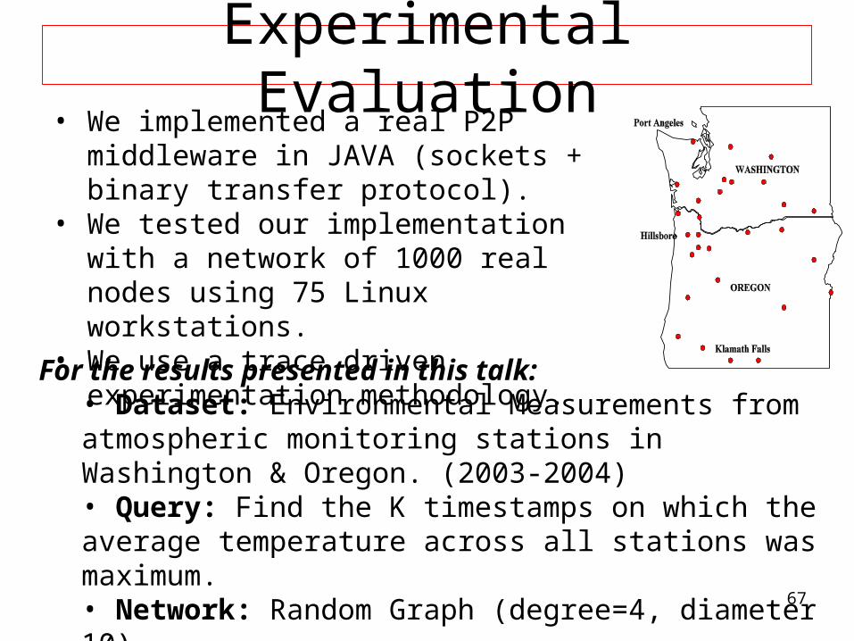
Experimental Evaluation• We implemented a real P2P middleware in

JAVA (sockets + binary transfer protocol).• We tested our implementation with a

network of 1000 real nodes using 75 Linux workstations.

• We use a trace driven experimentation methodology.

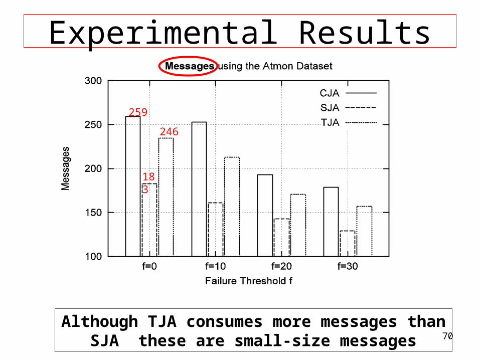
For the results presented in this talk:• Dataset: Environmental Measurements from atmospheric monitoring stations in Washington & Oregon. (2003-2004)• Query: Find the K timestamps on which the average temperature across all stations was maximum.• Network: Random Graph (degree=4, diameter 10)• Evaluation Criteria: i) Bytes, ii) Time, iii) Messages

68

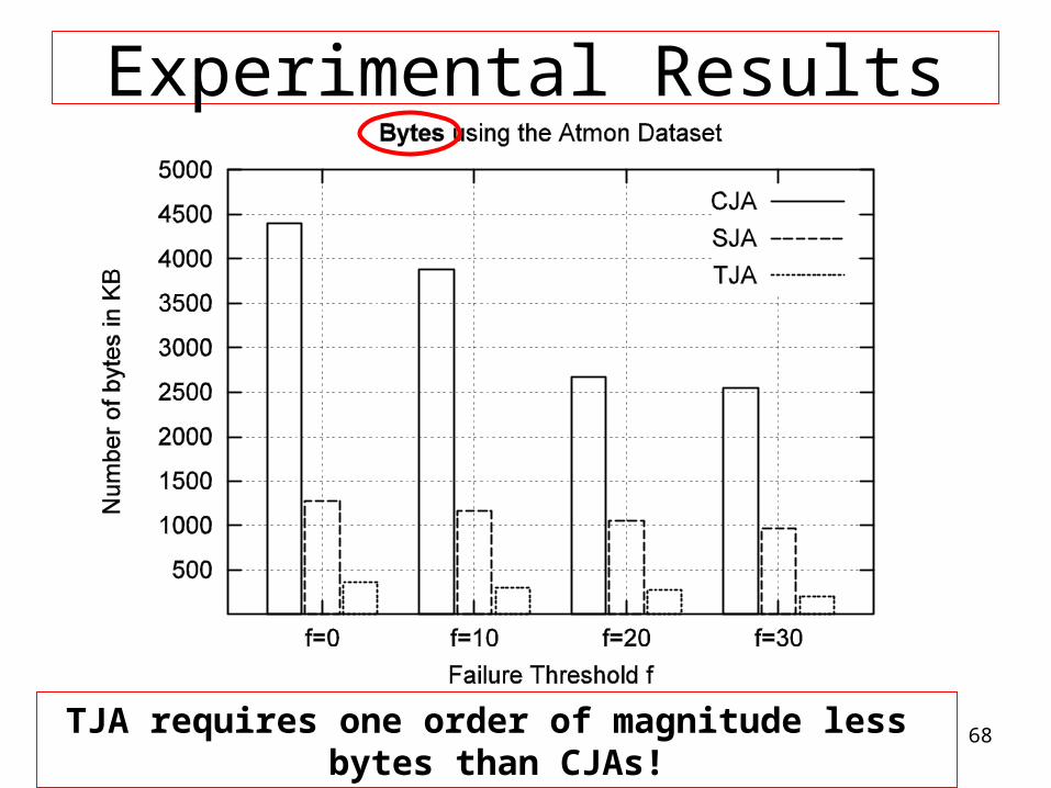
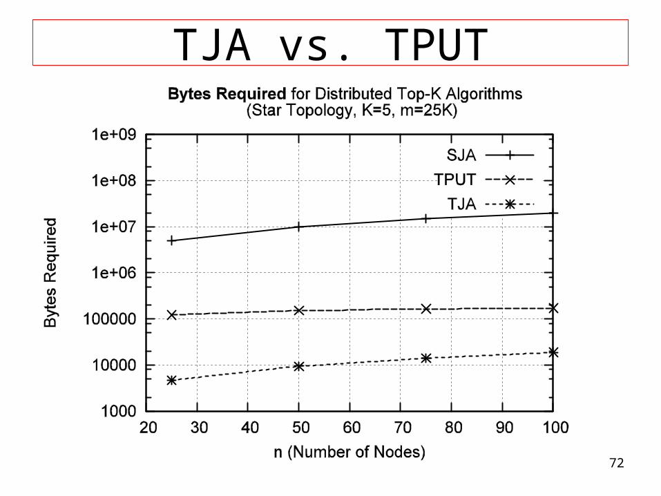
Experimental Results

TJA requires one order of magnitude less bytes than CJAs!

69

Experimental Results

TJA: 3.7sec [ LB:1.0sec, HJ:2.7sec, CL:0.08sec ] SJA: 8.2sec CJA:18.6sec

70

Experimental Results

259

183

246

Although TJA consumes more messages than SJA these are small-size messages

71

The TPUT Algorithm

v1 v2 v3 v4 v5o3, 99o1, 66o0, 63o2, 48o4, 44

o1, 91o3, 90o0, 61o4, 07o2, 01

o1, 92o3, 75o4, 70o2, 16o0, 01

o3, 74o1, 56o2, 56o0, 28o4, 19

o3, 67o4, 67o1, 58o2, 54o0, 35

P1 P2 P3

TOP-1

Phase 1 : o1 = 91+92 = 183, o3 = 99+67+74 = 240

τ = (Kth highest score (partial) / n) => 240 / 5 => τ = 48

Phase 2 : Have we computed K exact scores ?

Computed Exactly: [o3, o1] Incompletely Computed: [o4,o2,o0]

Drawback: The threshold is uniform (too coarse)

Q: TOP-1

o1=183, o3=240o3=405o1=363o2’=158o4’=137o0’=124

72

TJA vs. TPUT

73

Scalability Evaluation

• Remarks– By increasing the number of trajectories to 100,000

we observe that our algorithms continue to have a performance advantage.

100ΜΒ

100ΚΒ

1.6min

1 sec