Distributed Spectrum Sensing for Cognitive Radio Networks...

0090-6778 (c) 2018 IEEE. Personal use is permitted, but republication/redistribution requires IEEE permission. See http://www.ieee.org/publications_standards/publications/rights/index.html for more information.

This article has been accepted for publication in a future issue of this journal, but has not been fully edited. Content may change prior to final publication. Citation information: DOI 10.1109/TCOMM.2018.2880902, IEEETransactions on Communications

1

Distributed Spectrum Sensing for Cognitive RadioNetworks Based on the Sphericity Test

Peter J. Smith, Fellow, IEEE, Rajitha Senanayake, Member, IEEE, Pawel A. Dmochowski, Senior Member, IEEE,and Jamie S. Evans, Senior Member, IEEE

Abstract—We consider spectrum sensing in a cognitive radionetwork, with arbitrary numbers of primary and secondaryusers. Based on the sphericity test, we first analyze centralizedspectrum sensing where all the data available at the secondaryusers are combined for the signal detection of primary users.We derive accurate approximations for the false alarm anddetection probabilities which are also compared against theapproximations already available in literature. Next, we analyzedistributed spectrum sensing where only partial data from eachsecondary user is used in the signal detection of primary users.Two novel techniques namely, the multisample sphericity test andmeta analysis, are proposed and analyzed. Instead of sending allthe raw data received at the secondary user terminals, in themultisample sphericity test and meta analysis only one or two realnumbers are required to be sent to a central processor to make adecision about the presence of primary users. Accurate analyticalexpressions on the false alarm and detection probabilities arederived and numerical examples are provided to verify theiraccuracy. Receiver operating characteristic (ROC) curves are alsopresented to compare the performance of the proposed methods.

Index Terms—

Cognitive radio, distributed spectrum sensing, sphericity test.

I. INTRODUCTION

In view of the radio spectrum’s scarcity, it is necessary tofind new techniques for its efficient use in wireless commu-nications. In [1], it was revealed that some frequency bandsin the radio spectrum are largely unoccupied most of thetime. Cognitive radio is a promising technology that canbe used to improve radio spectrum utilization, by allowingunlicensed secondary users to share the spectrum resourcesof licensed primary users [2]–[7]. One principal requirementof this approach is that secondary user transmission does notcause intolerable interference to the primary users. This isachieved by the secondary users’ ability to detect the presenceof primary users, which is commonly referred to as spectrum

Peter J. Smith and Pawel A. Dmochowski are with Victoria Uni-versity of Wellington, New Zealand (email: [email protected],[email protected]).

Rajitha Senanayake and Jamie S. Evans are with The Univer-sity of Melbourne, Australia (email: [email protected],[email protected]).

Copyright (c) 2013 IEEE. Personal use of this material is permitted.However, permission to use this material for any other purposes must beobtained from the IEEE by sending a request to [email protected].

Manuscript received June 21, 2018; revised August 20, 2018; acceptedNovember 5, 2018. The review of this paper was coordinated by Dr. KyeongJin Kim.

This work is supported in part by the Australian Research Council(ARC) through the Discovery Early Career Researcher (DECRA) AwardDE180100501 and the Discovery Project (DP) DP140101050.

sensing. If no primary users are detected, the secondary usersare allowed to utilize the primary user’s licensed spectrum.

A. Related work and MotivationSpectrum sensing acts as an important tool in detecting the

so called spectrum holes, i.e., idle frequency bands that aretemporarily unused by the corresponding primary users, toefficiently deliver secondary user data, while protecting thecommunication quality of the primary user [8]. It has alsobeen included in the IEEE 802.22 standard, built on cognitiveradio techniques [9].

Several spectrum sensing techniques have been pro-posed in the literature including energy-based detectors [10],[11], eigenvalue-based spectrum sensing techniques [12]–[14],matched-filter based detectors [15] and covariance based spec-trum sensing techniques [16], etc. The energy-based detectorsare usually simple to implement, but they require knowledgeof the effective noise variance. In the present work, wefocus on eigenvalue-based spectrum sensing which does notrequire knowledge of the noise variance and offers remarkablyimproved performance for specific signal categories. In theliterature, many optimal eigenvalue-based spectrum sensingtechniques have been proposed and analysed under the as-sumption of a single active primary user [12]–[14]. However,in cellular systems the existence of multiple, simultaneouslytransmitting primary users is a prevailing condition and verylittle is known about performance under the presence ofmultiple primary users.

For such systems, a novel spectrum sensing algorithm,based on the sphericity test, has been proposed in [17].The authors use the optimal generalized likelihood ratio test(GLRT) paradigm and simulate the false alarm and detectionprobabilities. However, no analytical derivation relating to theperformance measures was presented. In [18], the authorsadopt the same model as in [17] and derive analytical formulaeto approximate the false alarm and detection probabilities inthe presence of multiple primary users. The approximation wasderived by matching the moments of test statistics to a Betadistribution. For the special case of only two secondary usersthe approximations in [18] reduce to the exact performancemeasures. In [19] and [20], the authors derive exact expres-sions for the moments of the GLRT statistic, and show thatthe normalized GLRT statistic converges in distribution to aGaussian random variable when the number of antennas andobservations grow large at the same rate.

While the optimal GLRT technique considered in [17]–[20] exhibits high detection performance, it requires a central



2

processor that gathers and processes the raw data received byall the secondary user terminals. This centralized architecturelimits the applicability of the GLRT technique to large net-works due to the resulting communication and computationburden. In order to overcome this problem, we are motivated toconsider more decentralized spectrum sensing techniques thatrequire only partial information to be exchanged between thesecondary users and the central processor. More specifically,we consider cases where the secondary users process the datalocally at the terminal, and share the processed data with thecentral processor to make the final decision.

B. Contributions

In this paper, we consider a general cognitive radio systemwith an arbitrary number of primary and secondary userterminals. Based on the sphericity test and the GLRT statisticwe investigate the detection performance of centralized anddecentralized spectrum sensing. Our novel contributions aredetailed as follows:

• Under centralized spectrum sensing we derive easy-to-evaluate closed-form approximations for the false alarmand the detection probabilities. Based on numerical ex-amples, we illustrate the accuracy of our approximationsand compare them against the analytical approximationsin [18] and [20].

• Under distributed spectrum sensing we propose two noveltechniques, namely, the multisample sphericity test andmeta analysis. In the multisample sphericity test each sec-ondary user calculates and sends only two real numbers,specifically, the trace and the determinant of the samplecovariance matrix, to detect the primary user signal.Under this scheme, we derive easy-to-evaluate, closed-form approximations for the false alarm and detectionprobabilities when the secondary users are subject toequal or unequal noise variances.

• In meta analysis each secondary user is required tocalculate and send only one real number, i.e., the extremeprobability value, more commonly known as the p-value,of the current test statistic. Under this technique also, wederive an easy-to-evaluate, closed-form approximation forthe false alarm probability.

• Furthermore, we compare the performance of the noveltechniques with other simple binary fusion methods,where each secondary user terminal makes a binarydecision about the presence of primary users and allthe decisions are simply combined through binary ANDor OR operation at the central processor. Under binaryfusion techniques also, we conduct a rigorous theoreticalanalysis by deriving closed-form approximations for thetest statistics distributions under both hypothesis.

• We present extensive numerical examples to illustrate theaccuracy of our results. Using the receiver operating char-acteristics (ROC), curves we compare the performanceof the proposed techniques. We observe that both themultisample sphericity test and meta analysis have similarperformance even though meta analysis requires only halfthe amount of information sent to the central processor.

The rest of the paper is organized as follows. In Section II wepresent the system model and outline the sphericity test basedcentralized test statistics. The theoretical analyses on derivingthe false alarm and detection probabilities are also presented.In Section III, we present the novel techniques of multisamplesphericity test and meta analysis, and analyze the false alarmprobability and detection probabilities. We also compare theperformance of different distributed spectrum sensing tech-niques based on ROC curves and present numerical examples.The paper is concluded in Section IV.

II. CENTRALIZED SPECTRUM SENSING

We consider a standard wireless communications systemwith P primary user terminals and M secondary user ter-minals. The secondary user terminals are tasked with coop-eratively determining the presence of primary users and thesecondary user terminal m is equipped with Qm antennassuch that, K =

∑Mm=1 Qm. In this system, each secondary

user terminal is connected to a central processor1, that coop-eratively detects the presence of primary users. The amountof information exchanged to the central processor could varydepending on the type of spectrum sensing technique used.This detection problem can be formulated as a binary hypoth-esis test, where the null hypothesis, H0, denotes the absenceof primary users and the non-null hypothesis, H1, denotes thepresence of primary users. Under centralized spectrum sensingwe assume that all the signals received at the secondary userterminals are available at the central processor. As such, then-th sample vector, xn, received at the central processor canbe modeled as

H0 : xn = wn no primary users presentH1 : xn = Hs+wn primary users present, (1)

where s = [s1, s2, . . . , sP ]T is the P × 1 data vector, which

contains the zero mean transmitted symbols from the Pprimary users, wn is the K × 1 additive white Gaussiannoise vector at the n-th sample with E[wnw

†n] = σ2IK and,

H = [h1,h2, . . . ,hP ] is the K × P channel matrix betweenthe P primary users and K receive antennas. We collect N in-dependent and identically distributed sample vectors such thatthe observed received signal matrix is X = [x1,x2, . . . ,xN ].Similar to [18], we assume that the channel H remainsconstant during this time. Note that unless otherwise specified,the results in this paper do not assume a specific distributionfor H. We also assume that the primary users signal followsan independent and identically distributed zero mean Gaussiandistribution and is uncorrelated with the noise.

A. Sphericity TestLet us define the sample covariance matrix R = XX†

such that when no primary users are present R follows anuncorrelated complex Wishart distribution with populationcovariance matrix

Σ =E[XX†]

N= σ2IK . (2)

1One of the secondary user terminals could be selected as the centralprocessor.



3

When primary users are present, for a given H, R followsa correlated complex Wishart distribution with populationcovariance matrix

Σ =P∑i=1

γihih†i + σ2IK , (3)

where γi = E[sis†i ] defines the transmission power of the i-th primary user. Thus, the hypothesis testing in (1) can berearranged to test the structure of the population covariancematrix Σ as

H0 : Σ = σ2IK no primary users present

H1 : Σ ≻ σ2IK primary users present, (4)

where A ≻ B denotes that A−B is a positive definite matrix.Note that no a priori knowledge on H, P and σ2 is assumed atthe secondary user terminals. The most critical information forthe secondary user is whether or not there are active primaryusers and the number of active users is not relevant. As such,we reject H0 if we have reason to believe that Σ departs fromthe spherical structure of Σ = σ2IK , which is the well-knownsphericity test [21], [22].

Different test criteria can be considered for the detectionproblem in (4). In this paper, we consider detectors of theNeyman-Pearson type, which involves comparing the gener-alized likelihood ratio to a user-designed detection threshold[23]. The generalized likelihood ratio used for determining H0

or H1 in (4) can be written as

L =supσ2∈R+L(X|σ2IK)

supΣ≻0L(X|Σ), (5)

where L(X|σ2IK) is the likelihood function of the observationmatrix under hypothesis H0 and L(X|Σ) is the likelihoodfunction of the observation matrix under hypothesis H1.Maximizing these likelihoods over the unknown parameters,i.e., finding the maximum likelihood estimates of σ2 underH0, and of σ2, γ1, γ2, . . . , γP and H under H1, results in theGLRT statistic [24]

TS =|R|(

1K tr(R)

)K . (6)

More details on the derivation of TS can be found in [18],[24]. Now, to determine H0 or H1 admits

TS ≷H0

H1ζ, (7)

where ζ is a user-specified detection threshold. Thus, thecentral processor calculates TS and declares that the primaryuser signals are present if TS < ζ, while no primary usersignals are believed to be present if TS > ζ.

B. Performance Measures

We consider two performance measures for the sphericitytest based detection, namely, the false alarm probability de-noted by Pfa and the detection probability denoted by Pd. Inthe following, we present the analytical results of those per-formance measures in closed-form expressions. We note thatunder centralized spectrum sensing approximate expressions

for the false alarm probability and detection probability arederived in [18], [20]. In [18], the test statistic is approximatedby a beta variable based on the moments of the distributions in-volved. In [20], the inverse of the test statistic is approximatedusing a Gaussian random variable. In the present paper, wederive alternative approximations for Pfa and Pd that are moreaccurate and yet easy-to-evaluate. In addition to the simplicity,our results are based on chi-squared (for Pfa) and normal(for Pd) approximations, which have a rigorous mathematicalbasis in asymptotic expansions as shown in [24, pg. 436] and[22, pg. 351], respectively. Numerical examples are presentedcomparing our results with the results in [18], [20].

1) Probability of false alarm: The false alarm probabilityis the probability of wrongly declaring H1, i.e., H1 is chosengiven that H0 is the true hypothesis. It can be defined as

Pfa = Pr[TSH0 ≤ ζ], (8)

where TSH0 is TS defined under hypothesis H0. From (8),note that Pfa is the CDF of TSH0 , evaluated at ζ which canbe denoted by FTSH0

(ζ). The threshold ζ should be carefullychosen such that Pfa is small and it can be calculated bynumerically inverting FTSH0

(ζ), i.e.,

ζ = F−1TSH0

(Pfa). (9)

In order to analyse Pfa, first we use the result in [18, eq.(35)] to find the exact moments of the N -th power of TSH0 ,i.e., TSN

H0, as

E[TSnNH0

] = KKn Γ(NK)

Γ(NK + nNK)

K∏k=1

Γ(N + nN − k + 1)

Γ(N − k + 1),

(10)

where n denotes the n-th moment and Γ(·) denotes the gammafunction [25, eq. (8.310)]. Next, we proceed to compare thesemoments with [24, Section 8.5.1, eq. (1)]. We observe thatthe expression in [24, Section 8.5.1, eq. (1)] reduces to (10)

when the constant K = Γ(NK)(∏K

k=1 Γ(N + 1− k))−1

,b = 1, a = K, y1 = NK, xk = N ∀ k ∈ {1, 2, . . . , a},η1 = 0 and {−ξ1,−ξ2, . . . ,−ξa} = {0, . . . ,K}. Hence wecan directly apply the general theory of asymptotic expansionsin [24, Section 8.5.1] to derive an approximation to the CDFof −2Nρ ln(TSH0) under the null hypothesis as

Pr[−2ρ ln(TSH0) ≤ x] ≈ Pr[χ2f ≤ x], (11)

where f = K2 − 1, ρ = N − 1+2K2

6K , and χ2f denotes a

chi-squared distribution with f degrees of freedom. Note thatthe full expression for the CDF of −2Nρ ln(TSH0) in [24]contains additional correction terms written in-terms of higherorder chi-squared distributions. For simplicity, we ignore thesecorrection terms and approximate Pr[−2Nρ ln(TSH0) ≤ x]by the chi-squared distribution in (11). We also note that thisresults can be obtained by using [26], [27]. Following simplemathematical manipulations (11) can be expressed as

Pr[

TSH0 ≥ exp

(− x

2Nρ

)]≈ Pr[χ2

f ≤ x]. (12)



4

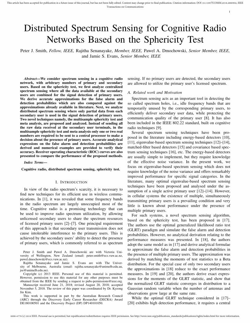
Fig. 1. Probability of false alarm vs the detection threshold for centralizedspectrum sensing.

Hence, we can derive an approximation for the CDF of TSH0

as

Pr[TSH0 ≤ x] ≈ 1− Pr[χ2f ≤ −2Nρ ln(x)]. (13)

Thus, Pfa for centralized spectrum sensing can be approxi-mated as

Pfa ≈ 1− Pr[χ2f ≤ −2Nρ ln(ζ)]. (14)

Comparing (14) with [18, eq. (17)] and [20, eq. (11)] we noticethat our results has a much simpler form and is very easy toevaluate.

Fig. 1 plots the Pfa versus the detection threshold ζ for dif-ferent numbers of secondary user terminals, by setting M = 4and 5. The secondary use terminals are allocated Qm = 2antennas each. We also change the number of observations,by setting N = 20 and 100. For each simulation trial, thenoise components are drawn from an independent complexGaussian distribution. The simulation curves are generatedbased on Monte-Carlo simulation, while the analytical curvesare generated using the approximation in (14). The figureillustrates extremely close agreement between the analyticalapproximation and the simulation curves. For a given detectionthreshold, an increase in M results in an increase in Pfa. Wealso compare these results with the beta and Gaussian approx-imations in [18] and [20]2, respectively. We observe that whencompared to the accuracy of our analytical approximation, thebeta approximation in [18, eq. (17)] is slightly loose in thelower tail when N = 20 and, the Gaussian approximation in[20, eq. (11)] is slightly loose in the lower tail when N = 100.

2In Fig. 1 we plot the Gaussian approximation in [20], without thecorrection terms. We agree that adding the correction terms will makethe approximation more accurate, but the complexity of the approximationincreases as it requires the calculation of the third and the fourth centralmoments of X . Therefore, to keep the complexity comparable with (14) and[18, eq. (17)] we ignore the correction terms in [20, eq. (11)].

0.15 0.2 0.25 0.3 0.35 0.4 0.45 0.5

ζ

10-2

10-1

100

Pd

Simulation

Analytical

Beta Approximation in [18]

Gaussian Approximation in [20]

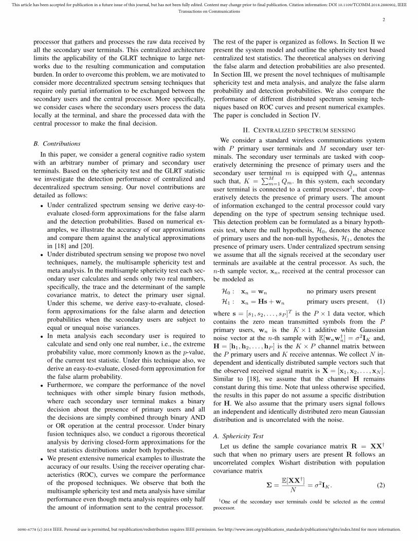
Fig. 2. Probability of detection vs the detection threshold for centralizedspectrum sensing.

2) Probability of detection: The detection probability is theprobability of declaring correctly H1, i.e., H1 is chosen giventhat H1 is the true hypothesis. It can be defined as

Pd = Pr[TSH1 ≤ ζ]

= FTSH1(ζ), (15)

where TSH1 is TS defined under hypothesis H1 and FTSH1(ζ)

is the CDF of TSH1 evaluated at ζ.In order to analyse Pd, we first use [22, Theorem 8.3.9] to

learn that under H1, the distribution of the variable ln(TSH1)is closely Gaussian. This is also confirmed by the Monte-Carlosimulations which showed that the empirical distribution ofln(TSH1) approaches a Gaussian as the number of observa-tions grows large. Motivated by these observations we proceedto approximate the CDF of TSH1 using a Gaussian distributionas

Pr[TSH1 ≤ x] ≈ Pr[Z ≤ ln(x)], (16)

where Z ∼ N (µ, ν2), µ = K2 ln(m2)− 2K ln(m1) and ν2 =

K2 ln(m2)−2K2 ln(m1) denote the mean and the variance ofthe Gaussian distribution. The terms m1 and m2 denote thefirst and the second moments of TS−1/K

H1, respectively, and

are given by (17) and (18) at the top of the next page, withσ2 < λ1 ≤ λ2 ≤ . . . ≤ λK < ∞ denoting the eigenvalues ofHH† + σ2IK . A detailed proof of (16) is given in AppendixA.

Based on (16), Pd for centralized spectrum sensing can beapproximated as

Pd ≈ Pr[Z ≤ ln(ζ)]. (19)

Comparing (19) with [18, eq. (25)] and [20, eq. (11)] we noticethat our result has a much simpler form and is trivial evaluate.

Fig. 2 plots Pd versus the detection threshold ζ for a networkwith P = 3 primary users, M = 5 and N = 100. Thesecondary user terminals are allocated Qm = 2 antennas each.



5

m1 =

(NK − 1

K2

) K∏k=1

λ−1/Kk

K−1∏j=0

Γ(N −K − 1/K + 1 + j)

Γ(N −K + 1 + j)

K∑i=1

λi, (17)

m2 =

(NK − 2

K3

) K∏k=1

λ−2/Kk

K−1∏j=0

Γ(N −K − 2/K + 1 + j)

Γ(N −K + 1 + j)

K∑i=1

λi +

(N − 2

K

)( K∑i=1

λi

)2 , (18)

We fix the transmit power values as γ1 = γ2 = γ3 = −10dB and plot the detection probability for three differentchannel realizations. The simulation curves are generatedbased on Monte-Carlo simulation, while the analytical curvesare generated using the approximation in (19). The figureillustrates close agreement between the approximation and thesimulation curves. We also compare this results with the betaand Gaussian approximations in [18] and [20]. We observethat the approximation in [20] and our result have very closeperformance as the distributions of both 1/TSH1 and ln(TSH1)are closely Gaussian. Observing the lower tail of the plots,we also understand that the accuracy of each approximationdepends on the random channel realization that is selected.

III. DECENTRALIZED SPECTRUM SENSING

In this section, we consider decentralized spectrum sensing.Under the centralized spectrum sensing we assume that all thesignals received at secondary user terminals are received at thecentral processor. However, centralized spectrum sensing is notvery suitable for practical implementations of cognitive radionetworks. This is because calculating TS requires the sharingof all raw data received at the M secondary user terminalswith the central processor, producing considerable networkoverhead. Based on the sphericity test and the GLRT statis-tic, in the following we analyze two new spectrum sensingtechniques namely, the multisample sphericity test and metaanalysis that require the exchange of only partial information,with the central processor. Furthermore, we investigate thesimple binary fusion technique and compare the performance.

We consider the same system model as described in SectionII. Under this distributed setup we define the two hypotheses,H0 and H1, for sphericity as

H0 : Σm = σ2IQm for all m ∈ {1, 2, . . . ,M},H1 : Σm ≻ σ2IQm for at least one m ∈ {1, 2, . . . ,M},

(20)

where Σm = E[XmX†m]/N is the population covariance

matrix with Xm denoting the Qm ×N observed data matrixat the secondary user terminal m.

A. Multisample sphericity test

In this subsection we present the first novel distributedspectrum sensing technique named, the multisample sphericitytest. Based on the distributed setup, the generalized likelihood

ratio for determining H0 or H1 defined in (20) can be writtenas

L =supσ2∈R+L(X1,X2, . . . ,XM |σ2IQ1 , . . . , σ

2IQM)

supΣ1≻0,...,ΣM≻0L(X1,X2, . . . ,XM |Σ1, . . . ,ΣM ),

(21)

where L(X1,X2, . . . ,XM |σ2IQ1 , . . . , σ2IQM ) is the likeli-

hood function of the observation matrices under hypothesisH0 and L(X1,X2, . . . ,XM |Σ1, . . . ,ΣM ) is the likelihoodfunction of the observation matrices under hypothesis H1. Fol-lowing the derivation methodology in [22, Theorem 8.3.2] andmaximizing these likelihoods over the unknown parameters,the modified GLRT statistic for testing the above hypothesiscan be obtained as

MSTS =

∏Mm=1 |Rm|(

1K

∑Mm=1 tr(Rm)

)K , (22)

where Rm = XmX†m is the sample covariance matrix at

the secondary user terminal m. Note that the MSTS in (22)reduces to a similar form to TS in (6) when M = 1.Thus, instead of sending the whole matrix Xm, which isthe case with the centralized spectrum sensing, the multi-sample sphericity test requires the secondary user terminalm to calculate |Rm| and tr(Rm) and share with the centralprocessor the two real numbers. The central processor collectsall matrix determinants and traces from the M secondary userterminals and calculates the global MSTS according to (22).We determine H0 or H1 in the multisample sphericity test as

MSTS ≷H0

H1ζ. (23)

In order to analyse the performance of the multisamplesphericity test, we next proceed to derive an analytical ex-pression for Pfa and Pd based on (22).

1) Probability of false alarm: Based on [18], we first writethe exact n-th moment of the N -th power of MSTS under H0

as

E[(MSTSH0)Nn] =

KnNKΓ(NK)

Γ(NK + nNK)

M∏m=1

Qm∏q=1

Γ(N + nN + 1− q)

Γ(N + 1− q), (24)

where MSTSH0 denotes the MSTS under H0, Similar toSection II-B1, next we proceed to compare (24) with [24,Section 8.5.1, eq. (1)]. We observe that the expressionin [24, Section 8.5.1, eq. (1)] reduces to (24) when the

constant K = Γ(NK)(∏M

m=1

∏Qm

q=1 Γ(N + 1− q))−1

,



6

0.85 0.9 0.95 1ζ

0

0.2

0.4

0.6

0.8

1

Pfa

AnalyticalSimulation

Scenario 02

Scenario 03

Scenario 01

Fig. 3. Probability of false alarm vs the detection threshold for scenario 01,02 and 03 with N = 200, M = 5.

b = 1, a = K, y1 = NK, xk = N ∀ k ∈{1, 2, . . . , a}, η1 = 0 and {−ξ1,−ξ2, . . . ,−ξa} ={0, . . . , Q1 − 1, 0, . . . , Q2 − 1, . . . , 0, . . . , QM − 1}. Thus,we follow the expansion method in [24, Section 8.5.1] andderive an approximation to the CDF of −2ρ ln(MSTSH0)under the null hypothesis as

Pr[−2ρ ln(MSTSH0) ≤ x] ≈ Pr[χ2f≤ x], (25)

where f =∑M

m=1 Q2m−1, ρ = N− 1+K2−2K

∑Mm=1 Q3

m

6K(1−∑M

m=1 Q2m)

. Fol-lowing simple mathematical manipulations an approximationfor the CDF of MSTS can be derived as

Pr[MSTSH0 ≤ x] ≈ 1− Pr[χ2f≤ −2ρ ln(x)]. (26)

Thus, Pfa for the multisample sphericity test can be approxi-mated as

Pfa ≈ 1− Pr[χ2f≤ −2ρ ln(ζ)]. (27)

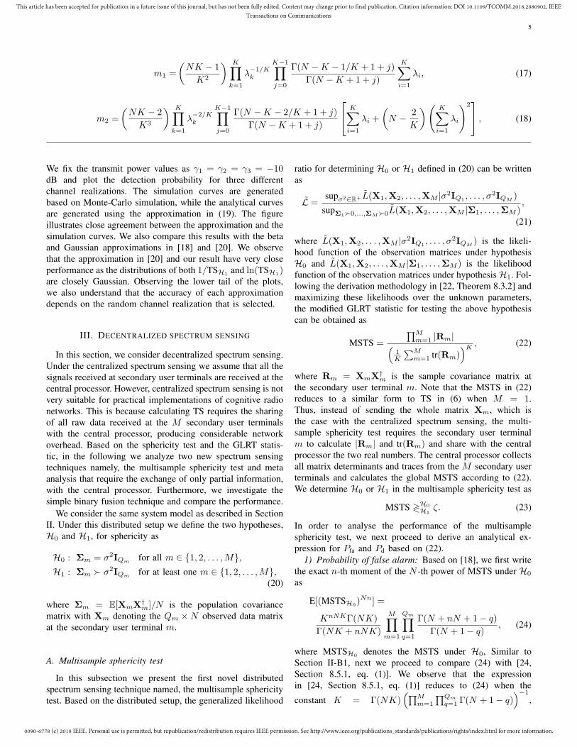
Fig. 3 plots Pfa versus the detection threshold ζ for differentnumber of antennas at each secondary user terminal. For fixedM = 5, N = 200, we consider the following three scenarios.In scenario 01, Q1 = 3, Q2 = 1 Q3 = 2, Q4 = 4 andQ5 = 2. In scenario 02, Q1 = 2, Q2 = 1 Q3 = 1, Q4 = 3and Q5 = 2, and in scenario 03, Qm = 1, ∀m ∈ {1, 2, . . . 5}.As such, the root mean square (RMS) value of the numberof antennas is 2.6, 1.67 and 1, respectively. As observed inthe conference vesion of this paper [28], the figure illustratesthat the approximation is very accurate for all three scenariosand for a given detection threshold the Pfa increases with theincreasing RMS value of Qm.

2) Probability of detection: We follow a similar ap-proach to Section II-B2 and approximate the distribution ofln(MSTSH1), where MSTSH1 denotes MSTS under H1, by

0.4 0.5 0.6 0.7 0.8 0.9 1

ζ

0

0.2

0.4

0.6

0.8

1

P d


N = 50, 100, 200

Fig. 4. Probability of detection vs the detection threshold for N = 50, 100and 200, with M = 2 and Qm = 3.

a Gaussian distribution with mean µ and variance ν2. Let usfirst define a new random variable X such that

X ≈ ln

(1

MSTSH1

), (28)

and X ∼ N (−µ, ν2). Based on (28), we can approximate thefirst and the second moments of MSTSH1 as

m1 = E[(

1

MSTSH1

)]≈ E[eX ] = e−µ+ ν2

2 , (29)

m2 = E

[(1

MSTSH1

)2]≈ E[e2X ] = e−2µ+2ν2

, (30)

where (29) and (30) are derived using the moment generatingfunction. Next, we take the ratio between (29) and (30) anddo some mathematical manipulations to derive approximateexpressions for µ and ν2 in terms of m1 and m2 as

µ ≈ ln(m2)− 2 ln(m1), (31)

ν2 ≈ 1

2ln(m2)− 2 ln(m1). (32)

We derive the exact expressions for m1 and m2 in AppendixC and the resultant closed-form expressions can be found in(81) and (84), respectively.

Thus, the CDF Of ln(MSTSH1) can be approximated by

Pr[ln(MSTSH1) ≤ x] ≈ Pr[Z ≤ x], (33)

where Z ∼ N (µ, ν2), µ and ν can be approximated bysubstituting (81) and (84) into (31) and (32), respectively.Based on (33), Pd for decentralized spectrum sensing withmultisample sphericity test can be approximated as

Pd ≈ Pr[Z ≤ ln(ζ)]. (34)

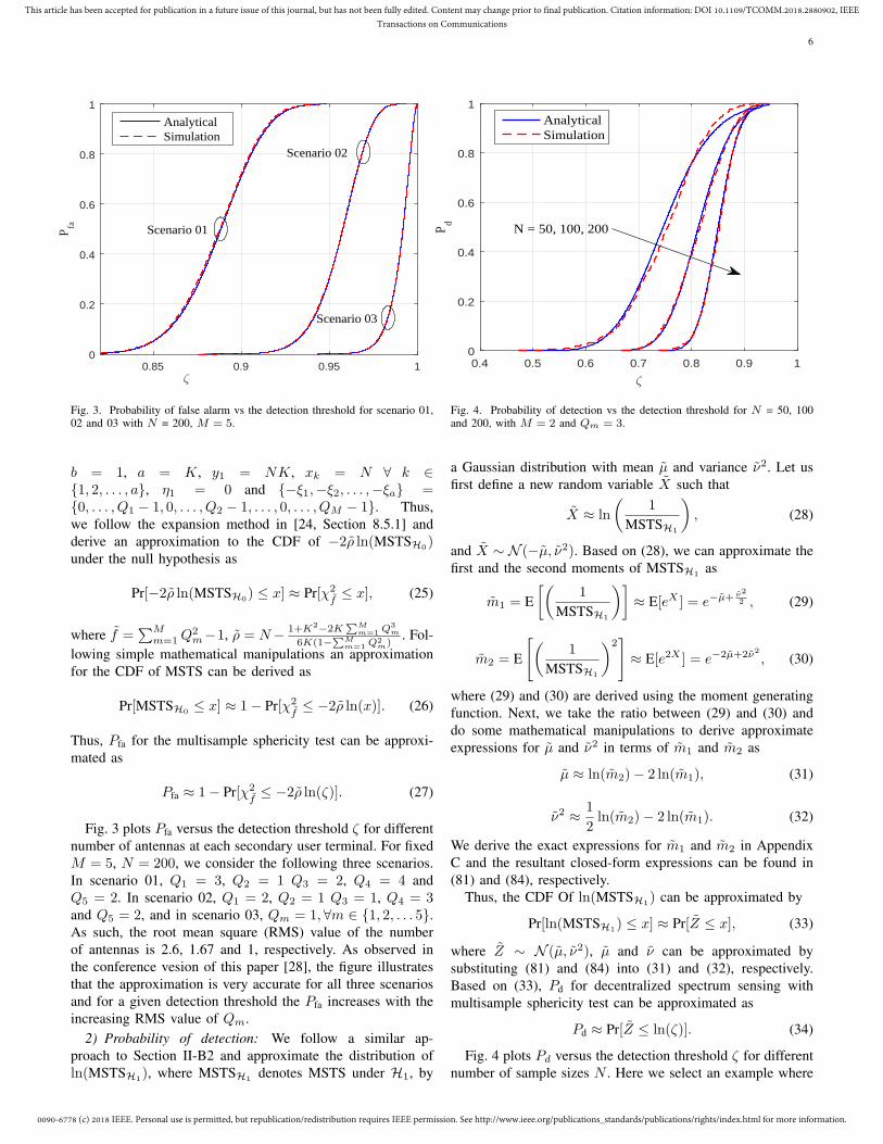
Fig. 4 plots Pd versus the detection threshold ζ for differentnumber of sample sizes N . Here we select an example where



7

0.75 0.8 0.85 0.9 0.95 1

ζ

0

0.2

0.4

0.6

0.8

1

Pfa


N = 50, 100, 200

Fig. 5. Probability of false alarm vs the detection threshold for N = 50, 100,and 200 with M = 4 and Qm = 2.

P = 2, M = 2, Q1 = Q2 = 3 and examine Pd forN = 50, 100 and 200. We fix the transmit power values toγ1 = γ2 = −10 dB. The simulation curves are generatedusing Monte-Carlo simulations while the analytical curves aregenerated using the approximation in (34). As the Gaussianapproximation is large sample based, we expect the approxi-mation to be more accurate when N is large. This is clearlyillustrated by the close agreement between the approximationand the simulation curves, especially when N = 100 and 200.

3) Multisample sphericity test with unequal noise variance:Under the distributed hypothesis testing in (20) we assumethat the secondary user terminals experience the same noisevariance. While this is a very common assumption in thecommunications literature, geographically separated secondaryuser terminals may experience different noise variances due totemperature changes and/or changes in the mechanical prop-erties they experience. In that case, the distributed hypothesistesting in (20) can be rearranged as

H0 : Σm = σ2mIQm for all m ∈ {1, 2, . . . ,M},

H1 : Σm ≻ σ2mIQm for at least one m ∈ {1, 2, . . . ,M},

(35)

where σ2m is the noise variance at secondary user terminal

m. The GLRT statistic for testing the above hypothesis canbe obtained by following the same derivation methodology in[22, Theorem 8.3.2] which results in

MSTS′ =M∏

m=1

|Rm|(1

Qmtr(Rm)

)Qm. (36)

As the new global test statistic in (36) takes a form differentto MSTS in (22), Pfa and Pd under unequal noise varianceslead to different approximations given by

Pfa ≈ 1− Pr[χ2f≤ −2ρ ln(ζ)], (37)

0.1 0.2 0.3 0.4 0.5 0.6 0.7 0.8 0.9

ζ

0

0.1

0.2

0.3

0.4

0.5

0.6

0.7

0.8

0.9

1

P d


N = 50, 100, 200

Fig. 6. Probability of detection vs the detection threshold for N = 50, 100,and 200 with M = 4 and Qm = 5.

where ρ = N −∑M

m=1

Q3m3 −K

6 −∑M

m=11

6Qm∑Mm=1 Q2

m−∑M

m=1 Qm−M, f =

∑Mm=1 Q

2m −

M and

Pd ≈ Pr[Z ≤ ln(ζ)

], (38)

where Z ∼ N(∑M

m=1 µm,∑M

m=1 ν2m

), µm = Qm

2 ln(m′2)−

2Qm ln(m′1) and ν2m = Q2

m ln(m′2)−2Q2

m ln(m′1). The terms

m′1 and m′

2 are given at the top of the next page by (39) and(40), respectively, with σ2

m < λm1 ≤ λm

2 ≤ . . . ≤ λmQm

<

∞ denoting the eigenvalues of HmH†m + σ2

mIQm and Hm

denoting the Qm × P channel matrix between the P primaryusers and the Qm receive antennas at secondary user terminalm. More details on the derivation of (37) and (38) are givenin Appendix B.

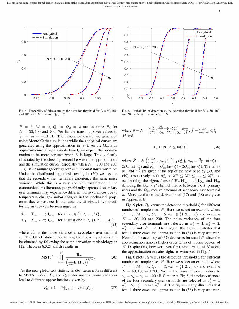
Fig. 5 plots Pfa versus the detection threshold ζ for differentnumber of sample sizes N . Here we select an example whereP = 3, M = 4, Qm = 2, ∀m ∈ {1, 2, . . . 4} and examineN = 50, 100 and 200. The noise variances of the foursecondary user terminals are selected as σ2

1 = 1, σ22 = 2,

σ23 = 3 and σ2

4 = 4. Once again, the figure illustrates thatfor all three cases the approximation in (37) is very accurate.Note that the accuracy of (37) decreases for small N , since theapproximation ignores higher order terms of inverse powers ofN . Despite this, however, even for a small value of N = 50,the approximation remains tight, as witnessed in Fig. 5.

Fig. 6 plots Pd versus the detection threshold ζ for differentnumber of sample sizes N . Here we select an example whereP = 3, M = 4, Qm = 5, ∀m ∈ {1, 2, . . . 4} and examineN = 50, 100 and 200. We fix the transmit power values toγ1 = γ2 = γ3 = −20 dB. Similar to Fig. 5, the noise variancesof the four secondary user terminals are selected as σ2

1 = 1,σ22 = 2, σ2

3 = 3 and σ24 = 4. The figure clearly illustrates that

for all three cases the approximation in (38) is very accurate.



8

m′1 =

(NQm − 1

Q2m

) Qm∏k=1

(λmk )−1/Qm

Qm−1∏j=0

Γ(N −Qm − 1/Qm + 1 + j)

Γ(N −Qm + 1 + j)

Qm∑i=1

λmi , (39)

m′2 =

(NQm − 2

Q3m

) Qm∏k=1

(λmk )−2/Qm

Qm−1∏j=0

Γ(N −Qm − 2/Qm + 1 + j)

Γ(N −Qm + 1 + j)

Qm∑i=1

λmi +

(N − 2

Qm

)(Qm∑i=1

λmi

)2 , (40)

B. Meta Analysis

In this subsection we present the second novel distributedspectrum sensing technique named meta analysis. Meta anal-ysis refers to the synthesis of data from multiple independenttests. Several techniques of meta analysis are available in theliterature. In this paper, we use the Fisher’s method whichcombines the results from several independent tests bearingupon the same overall hypothesis to produce a global teststatistic [29].

Similar to the multisample sphericity test, under this dis-tributed setup we can define the hypothesis H0 for sphericityas given in (20). Based on the measurements over the Ntime slots, each secondary user terminal calculates the extremevalue probabilities, commonly known as p-values. The p-valueat the secondary user terminal m can be written as

pm = Pr[TSm ≤ TSm|H0] (41)

where TSm = |Rm|( 1

Qmtr(Rm))

Qm, is the random variable repre-

senting the local GLRT at the secondary user terminal m andTSm is the current value of this test statistic. It is important tonote that the MSTS expression in (22) reduces to TSm whenM = 1. As such, we can follow the same steps as in thederivation of Pfa in (14) to find an analytical approximationfor pm as

pm ≈ 1− Pr[χ2fm ≤ −2ρm ln(TSm)], (42)

where fm = Q2m − 1, ρm = N − 1+Q2

m−2Q4m

6Qm(1−Q2m) .

Having computed the p-value, each secondary user terminalsends it to the central processor. Thus, instead of sendingthe whole matrix Xm, which is the case with the centralizedspectrum sensing, meta analysis requires each secondary userterminal to send a single real number. The central processorcollects all the p-values from the M secondary user terminalsand combines them according to Fisher’s method to producea global test statistic [29]

MATS = −2

M∑m=1

ln(pm). (43)

We determine H0 or H1 in the meta analysis test as

MATS ≶H0

H1ζ, (44)

where we reject the null hypothesis if MATS is larger than thethreshold ζ and reject the alternative hypothesis if MATS issmaller than ζ. In order to analyse the performance of the metaanalysis sphericity test, we now proceed to derive analyticalexpressions for Pfa based on (44). We would like to note that,

0 5 10 15 20 25ζ

0

0.2

0.4

0.6

0.8

1

Pfa


Q1 = 2, Q

2 = 3, Q

3 = 5, Q

4 = 4

Q1 = 2, Q

2 = 3, Q

3 = 5, Q

4 = 4, Q

5 = 2

M = 3, 4, 5

Q1 = 2,

Q2 = 3, Q

3 = 5

Fig. 7. Probability of false alarm vs the detection threshold for meta analysiswhen M = 3, 4 and 5.

due to the complexity of the derivation, we are unable to derivean analytical expression for Pd under meta analysis.

1) Probability of false alarm: While the CDF of the teststatistic in (43) is commonly available in the meta analysisliterature [29], for the sake of completeness we summarize thederivation of Pfa in the following. As the test statistic MATS isa sum of the logarithms of p-values, in order to derive the CDFof MATS we first focus on the CDF of − ln(pm). Following[29] we use the inverse transform method and write

TSm = F−1TSm,H0

(u), (45)

where FTSm,H0is the CDF of TSm under the hypothesis

H0 and u is uniformly distributed between 0 and 1. Basedon (45) we can express the p-value in (41) as pm =FTSm,H0

(F−1TSm,H0

(u)) = u. Hence, pm is also uniformlydistributed between 0 and 1 and the CDF of − ln(pm) has anexponential distribution. As the sum of M independent andexponentially distributed random variables has a standard chi-squared distribution with 2M degrees of freedom, we derivethe CDF of MATS as

Pr[MATS ≤ x] = Pr[χ22M ≤ x]. (46)

Thus, the exact closed-form expression for Pfa in meta analysiscan be derived as

Pfa = 1− Pr[χ22M ≤ ζ]. (47)



9

From (47) we learn that Pfa for meta analysis only dependson M and ζ, i.e., unlike in (14) for the multisample sphericitytest, it is not a function of the sensing duration N nor thenumber of secondary user antennas Qm. In the following, weuse numerical examples to illustrate the accuracy of (47).

While in this paper we consider only the GLRT statistic tocalculate the p-values, it is important to note that meta analysiscan be implemented with secondary user terminals operatingwith different test statistics. For example, the approach canbe used when one secondary user terminal uses the GLRTstatistic and another uses a simple power detector.

Fig. 7 plots the meta analysis Pfa versus the detectionthreshold ζ for different numbers of secondary user terminals,specifically M = 3, 4 and 5. In each case the secondaryuser terminals are allocated unequal number of antennas asnoted in the figure. The observation window is N = 200.We note that the parameters Qm and N do not effect the Pfain meta analysis. This is because under the null hypothesisthe p-values have a uniform distribution that varies betweenzero and one. The distribution of these tail probabilities donot change with Qm and N . Once again, the results obtainedusing the analytical expression in (47) agree closely with theMonte-Carlo simulations. Note that while the probability offalse alarm expression is exact, the p-values used to computeMATS use the chi-squared approximation in (42), which isthe cause of the slight discrepancy between the simulated andanalytical results.

C. Binary Fusion

In this subsection we present the third distributed spectrumsensing technique named binary fusion. In binary fusion eachsecondary user terminal performs a GLRT based on its ownmeasurements and makes a binary decision about the presenceof primary users. Based on (6), the individual test statistic ofsecondary user terminal m is given by TSm = |Rm|

( 1Qm

tr(Rm))Qm

.

To determine H0 or H1 at each secondary user terminal admits

TSm ≷H0

H1ζ. (48)

Each secondary user terminal then sends its binary decisionsto the central processor. As such, instead of sending the wholematrix Xm, in binary fusion the secondary user terminalm sends only one bit of information. The central processorcollects all M decisions and performs a binary AND or ORoperation to form the final decision.

1) Probability of false alarm: If the binary AND operationis used, the central processor declares H0 if at least onesecondary user terminal has declared H0. In other words, thecentral processor declares H1 if and only if all the secondaryuser terminals declared H1. As such, we can derive Pfa as

Pfa =M∏

m=1

Pr[TSmH0 < ζ]. (49)

Based on (14) we can derive an analytical approximation forPfa in (49) as

Pfa ≈M∏

m=1

[1− Pr[χ2fm ≤ −2ρm ln(ζ)]], (50)

0.95 0.96 0.97 0.98 0.99 1

ζ

0

0.2

0.4

0.6

0.8

1

Pfa


Binary AND

Binary OR

Fig. 8. Probability of false alarm vs the detection threshold for binary fusionwith N = 200, M = 4 and Qm = 2.

where fm = Q2m − 1, ρm = N − 1+Q2

m−2Q4m

6Qm(1−Q2m) .

Similarly, if the binary OR operation is used, the centralprocessor declares H0 if and only if all M secondary userterminals have declared H0. In other words, the central pro-cessor declares H1 if at least one secondary user terminal hasdeclared H1. Assuming independence of test statistics formedby each secondary user terminal, the overall Pfa is given by

Pfa = 1−M∏

m=1

[1− Pr[TSmH0 < ζ]] . (51)

Based on (14) we can derive an analytical approximation forPfa in (51) as

Pfa ≈ 1−M∏

m=1

Pr[χ2fm ≤ −2ρm ln(ζ)]. (52)

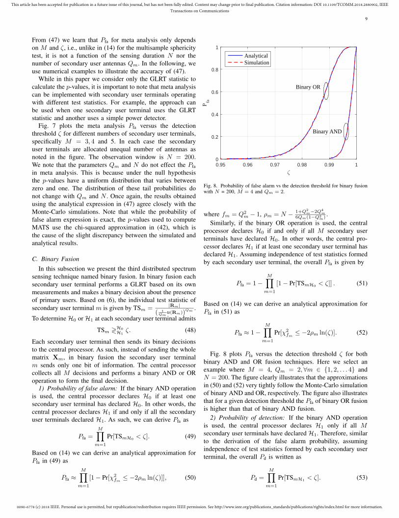
Fig. 8 plots Pfa versus the detection threshold ζ for bothbinary AND and OR fusion techniques. Here we select anexample where M = 4, Qm = 2,∀m ∈ {1, 2, . . . 4} andN = 200. The figure clearly illustrates that the approximationsin (50) and (52) very tightly follow the Monte-Carlo simulationof binary AND and OR, respectively. The figure also illustratesthat for a given detection threshold the Pfa of binary OR fusionis higher than that of binary AND fusion.

2) Probability of detection: If the binary AND operationis used, the central processor declares H1 only if all Msecondary user terminals have declared H1. Therefore, similarto the derivation of the false alarm probability, assumingindependence of test statistics formed by each secondary userterminal, the overall Pd is written as

Pd =M∏

m=1

Pr[TSmH1 < ζ]. (53)



10

Based on (19) we can derive an analytical approximation forPd in (53) as

Pd ≈M∏

m=1

Pr[Zm ≤ ln(ζ)], (54)

where Zm ∼ N (µm, ν2m).Similarly, if the binary OR operation is used, the central

processor declares H1 if at least one secondary user terminalhas declared H1. As such, we can derive Pd as

Pd = 1−M∏

m=1

[1− Pr[TSmH1 < ζ]] . (55)

Based on (19) we can derive an analytical approximation forPd in (55) as

Pd ≈ 1−M∏

m=1

[1− Pr[Zm ≤ ln(ζ)]] . (56)

Whilst not shown here, due to page page limitation, basedon numerical results we observe that the the approximation in(56) accurately follows the Monte-Carlo simulation of binaryOR fusion. The approximation in (54) is slightly loose in theupper tail regime, where Pd is close to one.

D. Comparison

In this subsection we investigate the performance of dis-tributed spectrum sensing schemes, by comparing the ROCcurves of multisample sphericity test, meta analysis, binaryfusion OR and binary fusion AND. In generating the ROCcurves we use our analytical approximations for Pfa and Pd,that was derived in Section III. For meta analysis the Pdperformance is generated using Monte-Carlo simulations. It isimportant to note that our accurate analytical approximationssave a significant amount of run time when compared to theMonte-Carlo simulations.

It is important to note that the amount of information ex-changed between the central processor and the secondary userterminals are different in each distributed sensing technique. Inthe multisample sphericity test each secondary user terminalexchanges two real numbers with the central processor, whilein meta analysis this amount is halved. In binary fusion, theamount of information exchanged is further reduced to a singlebinary data bit per secondary user terminal.

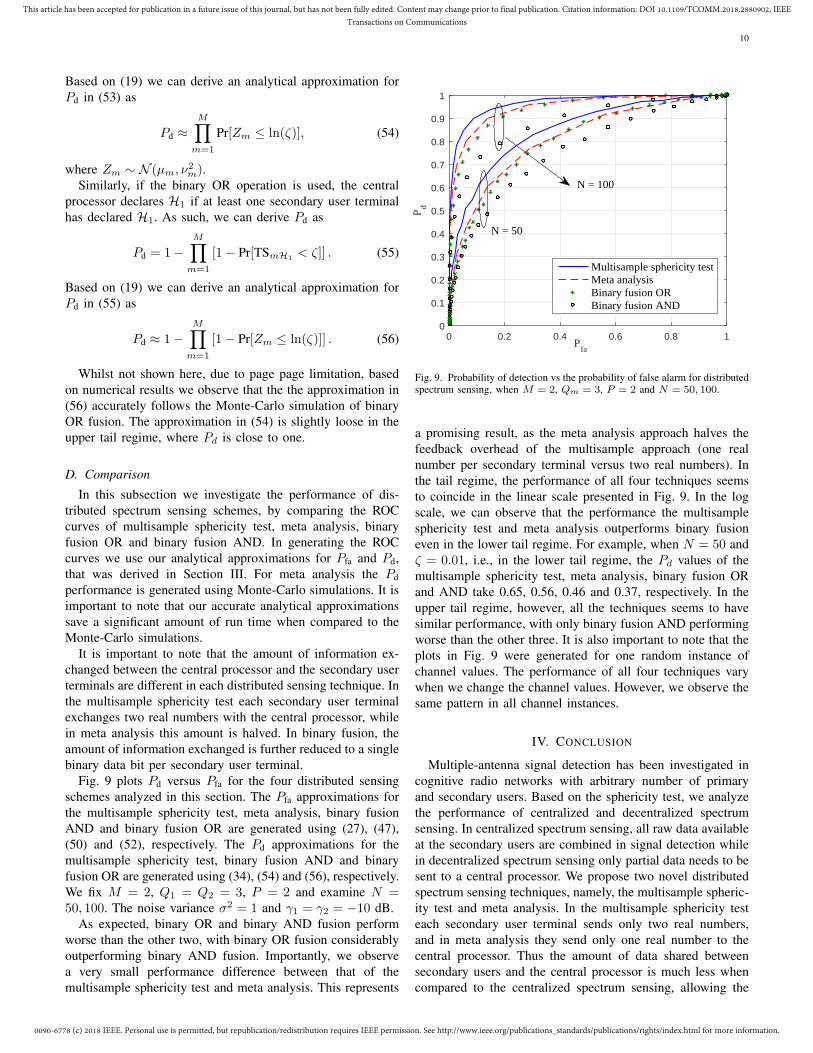
Fig. 9 plots Pd versus Pfa for the four distributed sensingschemes analyzed in this section. The Pfa approximations forthe multisample sphericity test, meta analysis, binary fusionAND and binary fusion OR are generated using (27), (47),(50) and (52), respectively. The Pd approximations for themultisample sphericity test, binary fusion AND and binaryfusion OR are generated using (34), (54) and (56), respectively.We fix M = 2, Q1 = Q2 = 3, P = 2 and examine N =50, 100. The noise variance σ2 = 1 and γ1 = γ2 = −10 dB.

As expected, binary OR and binary AND fusion performworse than the other two, with binary OR fusion considerablyoutperforming binary AND fusion. Importantly, we observea very small performance difference between that of themultisample sphericity test and meta analysis. This represents

0 0.2 0.4 0.6 0.8 1P

fa

0

0.1

0.2

0.3

0.4

0.5

0.6

0.7

0.8

0.9

1

Pd

Multisample sphericity testMeta analysisBinary fusion ORBinary fusion AND

N = 100

N = 50

Fig. 9. Probability of detection vs the probability of false alarm for distributedspectrum sensing, when M = 2, Qm = 3, P = 2 and N = 50, 100.

a promising result, as the meta analysis approach halves thefeedback overhead of the multisample approach (one realnumber per secondary terminal versus two real numbers). Inthe tail regime, the performance of all four techniques seemsto coincide in the linear scale presented in Fig. 9. In the logscale, we can observe that the performance the multisamplesphericity test and meta analysis outperforms binary fusioneven in the lower tail regime. For example, when N = 50 andζ = 0.01, i.e., in the lower tail regime, the Pd values of themultisample sphericity test, meta analysis, binary fusion ORand AND take 0.65, 0.56, 0.46 and 0.37, respectively. In theupper tail regime, however, all the techniques seems to havesimilar performance, with only binary fusion AND performingworse than the other three. It is also important to note that theplots in Fig. 9 were generated for one random instance ofchannel values. The performance of all four techniques varywhen we change the channel values. However, we observe thesame pattern in all channel instances.

IV. CONCLUSION

Multiple-antenna signal detection has been investigated incognitive radio networks with arbitrary number of primaryand secondary users. Based on the sphericity test, we analyzethe performance of centralized and decentralized spectrumsensing. In centralized spectrum sensing, all raw data availableat the secondary users are combined in signal detection whilein decentralized spectrum sensing only partial data needs to besent to a central processor. We propose two novel distributedspectrum sensing techniques, namely, the multisample spheric-ity test and meta analysis. In the multisample sphericity testeach secondary user terminal sends only two real numbers,and in meta analysis they send only one real number to thecentral processor. Thus the amount of data shared betweensecondary users and the central processor is much less whencompared to the centralized spectrum sensing, allowing the



11

application of these distributed spectrum sensing techniquesto larger cognitive radio networks. We have derived easy-to-compute and accurate analytical expressions for the falsealarm and the detection probabilities. Furthermore, we analyzethe performance of two simple fusion techniques based onbinary AND and binary OR combining and provide accurateapproximations for the false alarm and the detection probabil-ities. Extensive numerical examples are used to illustrate theaccuracy of our approximations. ROC curves are presented tocompare the performance of the proposed methods.

APPENDIX ADISTRIBUTION OF TS UNDER H1

Here we present the proof of (16). As described in II-B2,we are motivated to approximate the distribution of ln(TSH1)using a Gaussian distribution with mean µ and variance ν2.Let us first define a new random variable X such that

X ≈ ln

((1

TSH1

)1/K), (57)

and X ∼ N (−µ/K, ν2/K2). Based on (57), we can approx-imate the first and the second moments of (TSH1)

−1/K as

m1 ≈ e−µK + ν2

2K2 , (58)

m2 ≈ e−2µK + 2ν2

K2 , (59)

where (58) and (59) are derived using the moment generatingfunction. Next, we take the ratio between (58) and (59) anddo some mathematical manipulations to derive approximateexpressions for µ and ν2 in-terms m1 and m2 as

µ ≈ K

2ln(m2)− 2K ln(m1), (60)

ν2 ≈ K2 ln(m2)− 2K2 ln(m1). (61)

The exact expressions for the moments of (TSH1)−1/K can

be derived using [20, eq. (8)] which results in (60) and (61)for m1 and m2, respectively. Thus, the CDF Of ln(TSH1

) canbe approximated by

Pr[ln(TSH1) ≤ x] ≈ Pr[Z ≤ x], (62)

where Z ∼ N (µ, ν2). The expression in (62) can be rear-ranged as (16), completing the proof.

APPENDIX BDERIVATION OF (37) AND (38)

Here we present a detailed derivation of (37) and (38). Letus denote the random variable representing the local GLRTat the secondary user terminal m by TSm = |Rm|

( 1Qm

tr(Rm))Qm

.

The terms TSmH0and TSmH1

denote TSm under the nullhypothesis and the non-null hypothesis, respectively. It isstraightforward to derive the exact n-th moment of the N -th power of TSmH0

by simply replacing K in (24) by Qm.Noting that MSTS′ =

∏Mm=1 TSm, the n-th moment of the

N -th power of MSTS′ under the null hypothesis can then bederived as

E[(MSTS′H0

)Nn] =

M∏m=1

QnNQmm Γ(NQm)

Γ(NQm + nNQm)

Qm∏q=1

Γ(N + nN + 1− q)

Γ(N + 1− q), (63)

where MSTS′H0

denotes MSTS′ under H0. Similar to theequal noise case, next we proceed to compare (63) with [24,Section 8.5.1, eq. (1)]. We observe that the expression in[24, Section 8.5.1, eq. (1)] reduces to (63) when the constant

K =∏M

m=1 Γ(NQm)(∏M

m=1

∏Qm

q=1 Γ(N + 1− q))−1

,b = M , a = K, yj = NQj , xk = N ∀ k ∈{1, 2, . . . , a}, ηj = 0 and {−ξ1,−ξ2, . . . ,−ξa} ={0, . . . , Q1 − 1, 0, . . . , Q2 − 1, . . . , 0, . . . , QM − 1}. Thus,we follow the expansion method in [24, Section 8.5.1] andderive an approximation to the CDF of −2ρ ln(MSTS′

H0) as

Pr[−2ρ ln(MSTS′H0

) ≤ x] ≈ Pr[χ2f≤ x], (64)

which results in (37) for the false alarm probability of multi-sample sphericity test under unequal noise variances.

Under the non-null hypothesis, we use the result in (16)to first approximate the distribution of ln

(TSmH1

)using a

Gaussian distribution with mean µm and variance ν2m. Letus first define a new random variable Xm such that Xm ∼N (−µm/Qm, ν2m/Q2

m) and

Xm ≈ ln

( 1

TSmH1

)1/Qm . (65)

Based on (65), we can approximate the first and the secondmoments of

(TSmH1

)−1/Qm as

m′1 ≈ e

− µmQm

+ν2m

2Q2m , (66)

m′2 ≈ e

− 2µmQm

+2ν2

mQ2

m , (67)

where (66) and (67) are derived using the moment generatingfunction. Next, we take the ratio between (66) and (67) anddo some mathematical manipulations to derive approximateexpressions for µm and ν2m in-terms m′

1 and m′2 as

µm ≈ Qm

2ln(m′

2)− 2Qm ln(m′1), (68)

ν2m ≈ Q2m ln(m′

2)− 2Q2m ln(m′

1). (69)

The exact expressions for the moments of(TSmH1

)−1/Qm

can be derived using [20, eq. (8)] which results in (39) and (40)for m′

1 and m′2, respectively. Since MSTS′ =

∏Mm=1 TSm, we

can finally approximate the distribution of ln(MSTS′) using

a Gaussian distribution with mean∑M

m=1 µm and variance∑Mm=1 ν

2m and write

Pr[MSTS′H1

≤ x] ≈ Pr[Z ≤ ln(x)

], (70)

where here Z ∼ N(∑M

m=1 µm,∑M

m=1 ν2m

), µm =

Qm

2 ln(m′2)− 2Qm ln(m′

1). This results in (38) for the detec-tion probability of multisample sphericity test under unequalnoise variances.



12

APPENDIX CDERIVATION OF m1 AND m2

In this section, we derive an analytical expressions for thefirst and the second moments of 1

MSTSH1. From [18, eq. (40)],

we learn that the PDF of the sample covariance matrix at thesecondary user terminal m, is given by

f(Rm) =|Rm|N−Qm∆N,Qmexp

(tr(−Σ−1

m Rm))

|Σm|N, (71)

where ∆N,Qm = 1/(π

Qm2 (Qm−1)

∏Qm−1q=1 Γ(N − q)

). Based

on (71), we can write the r-th moment of 1MSTSH1

as

E[

1

MSTSrH1

]=

1

KKr

∫R1

. . .

∫RM

(∑Mm=1 tr(Rm)

)Kr

∏Mm=1 |Rm|r

×M∏j=1

|Rj |N−Qj∆N,Qj exp(tr(−Σ−1

j Rj))

|Σj |NdR1 . . . dRM .

(72)

Assuming that all the secondary user terminals have thesame number of antennas, i.e., Qm = Q ∀{1, 2, . . . ,M}, werearrange (72) as

E[

1

MSTSrH1

]

=1

KKr

M∏m=1

∆N,Q

|Σm|r∆N−r,Q

∫R1

. . .

∫RM

(M∑

m=1

tr(Rm)

)Kr

×M∏j=1

|Rj |N−Q−r∆N−r,Qexp(tr(−Σ−1

j Rj))

|Σj |N−rdR1 . . . dRM .

(73)

Identifying that the M -fold integral in (73) represents the

expected value of(∑M

m=1 tr(Rm))Kr

, we further simplify(73) as

E[

1

MSTSrH1

]=

1

KKr

(∆N,Q

∆N−r,Q

)M[

M∏m=1

1

|Σm|r

]

× E

( M∑m=1

tr(Rm)

)Kr . (74)

Based on (74), we next proceed to find m1. We set r = 1 in(74) and write

m1 =1

KK∏Q−1

j=0 (N − 1− j)M∏M

m=1 |Σm|

× E

( M∑m=1

tr(Rm)

)K . (75)

Note that the derivation of the expected value of 1MSTSH1

has

now reduced to deriving the K-th moment of∑M

m=1 tr(Rm).

Let us denote ωm = tr(Rm). To derive the K-th moment of∑Mm=1 ωm we use the multinomial expansion and write

E

( M∑m=1

ωm

)K

=∑

∑ij=K,0≤ij≤K

(K!

i1!i2! . . . iM !

) M∏m=1

E[ωimm

], (76)

where the product in (76) results from the independence ofωm. Note that ωm =

∑Qi=1

λmi χi

2 , where λmi denotes the i-

th eigenvalue of hmh†m + σ2

mIQm and χi denotes a randomvariable with the standard chi-squared distribution, with 2(N−1) degrees of freedom. Thus, we can express E

[ωimm

]as

E[ωimm

]=

∑∑

jq=im,0≤jq≤im

(im!

j1!j2! . . . jQ!

) ∏Qq=1(λ

mq )jqE

[χjqq

]2im

,

(77)

where (77) are derived by applying the multinomial expansion.Let us denote E

[χjqq

]by µ

(2N−2)jq

. The moments of a chi-squared variable is well-known and can be found in [30] as

µ(2N−2)q =

2jqΓ(jq +N − 1)

Γ(N − 1). (78)

We substitute (78) into (77), using which (76) can be re-expressed as

E

( M∑m=1

ωm

)K

=∑

∑ij=K,0≤ij≤K

[(K!

i1!i2! . . . iM !

) M∏m=1

Ξm,im

], (79)

where

Ξm,im =∑∑

jq=im,0≤jq≤im

[(im!

j1!j2! . . . jQ!

) ∏Qq=1(λ

mq )jqµ

(2N−2)q

2im

].

(80)

Substituting (79) into (75) we finally derive a closed-formexpression for m1 as

m1 =1

KK∏Q−1

j=0 (N − 1− j)M∏M

m=1 |Σm|

∑∑

ij=K,0≤ij≤K

×

[(K!

i1!i2! . . . iM !

) M∏m=1

Ξm,im

]. (81)



13

Based on (74), we next proceed to find m2. Following a sim-ilar approach to deriving the K-th moment of

∑Mm=1 tr(Rm)

we derive the 2K-th moment of∑M

m=1 tr(Rm) as

E

( M∑m=1

ωm

)2K

=∑

∑ij=2K,0≤ij≤2K

[((2K)!

i1!i2! . . . iM !

) M∏m=1

Θm,im

], (82)

where

Θm,im =∑∑

jq=im,0≤jq≤im

[(im!

j1!j2! . . . jQ!

) ∏Qq=1(λ

mq )jqµ

(2N−4)q

2im

],

(83)

and µ(2N−4)q =

2jqΓ(jq+N−2)Γ(N−2) . Substituting (82) into (74)

when r = 2, we derive a closed-form expression for m2 as

m2 =1[∏Q−1

j=0 (N − j − 1)M (N − j − 2)M]∏M

m=1 |Σm|2

× 1

K2K

∑∑

ij=2K,0≤ij≤2K

[((2K)!

i1!i2! . . . iM !

) M∏m=1

Θm,im

].

(84)

REFERENCES

[1] F. C. Commission, Spectrum policy task force, Rep. ET Docket no., pp.02135, Nov. 2002.

[2] B. Li, S. Li, A. Nallanathan, and C. Zhao, Deep sensing for futurespectrum and location awareness 5G communications, IEEE J. Sel. AreasCommun., vol. 33, pp. 13311344, Jul. 2015.

[3] S. Haykin, Cognitive radio: Brain-empowered wireless communications,IEEE J. Sel. Areas Commun., vol. 23, pp. 201220, Feb. 2005.

[4] I. F. Akyildiz, W. Y. Lee, M. C. Vuran, and S. Mohanty, A surveyon spectrum management in cognitive radio networks, IEEE Commun.Mag., vol. 46, pp. 4048, Jan. 2008.

[5] G. Staple and K. Werbach, The end of spectrum scarcity, IEEE Spectrum,vol. 41, pp. 4852, Mar. 2004.

[6] D. Cabric, Addressing feasibility of cognitive radios, IEEE Trans. SignalProcess., vol. 25, pp. 8593, Nov. 2008.

[7] J. M. Peha, Sharing spectrum through spectrum policy reform andcognitive radio, Proc. IEEE, vol. 97, pp. 708719, 2009.

[8] N. I. Miridakis, T. A. Tsiftsis, G. C. Alexandropoulos, and M. Debbah,Simultaneous spectrum sensing and data reception for cognitive spatialmultiplexing distributed systems, IEEE Trans. Wireless Commun., vol.16, pp. 33133327, Oct. 2017.

[9] C. Cordeiro, K. Challapali, and N. S. Shankar, IEEE 802.22: Thefirst worldwide wireless standard based on cognitive radios, in IEEEInt. Symp. New Frontiers Dynam. Spectrum Access Netw. (DySPAN),Baltimore, USA, Nov. 2005, pp. 328337.

[10] V. Kostylev, Energy detection of a signal with random amplitude, inIEEE International Conference on Communications (ICC), New York,NY, USA, USA, Aug. 2002, pp. 16061610.

[11] F. Digham, M. S. Alouini, and M. K. Simon, On the energy detection ofunknown signals over fading channels, in IEEE International Conferenceon Communications (ICC), May 2003, pp. 35753579.

[12] S. Kritchman and B. Nadlerg, Non-parametric detections of the numberof signals: Hypothesis testing and random matrix theory, IEEE Trans.Signal Process., vol. 57, pp. 39303941, Oct. 2009.

[13] A. Taherpour, M. N. Kenari, and S. Gazor, Multiple antenna spectrumsensing in cognitive radios, IEEE Trans. Wireless Commun., vol. 9, pp.814823, Feb. 2010.

[14] Y. Zeng, C. L. Koh, and Y. C. Liang, Maximum eigenvalue detection:theory and application, in IEEE International Conference on Communi-cations (ICC), Beijing, China, May 2008.

[15] S. Haykin, D. Thomson, and J. Reed, Spectrum sensing for cognitiveradio, Proc. IEEE, vol. 97, pp. 849877, May 2009.

[16] Y. Zeng and Y. C. Liang, Spectrum-sensing algorithms for cognitiveradio based on statistical covariances, vol. 4, pp. 18041815, May 2009.

[17] R. Zhang, T. J. Lim, Y. C. Liang, and Y. Zeng, Multi-antenna basedspectrum sensing for cognitive radios: A GLRT approach, IEEE Trans.Commun., vol. 58, pp. 8488, Jan. 2010.

[18] L. Wei and O. Tirkkonen, Spectrum sensing in the presence of multipleprimary users, IEEE Trans. Commun., vol. 60, pp. 12681277, May 2012.

[19] R. H. Y. Louie, M. R. McKay, and Y. Chen, Multiple-antenna signaldetection in cognitive radio networks with multiple primary user signals,in IEEE Int. Conf. Commun. (ICC) 2014, Sydney, Australia, Jun. 2014,pp. 49514956.

[20] D. M. Jimenez, R. H. Y. Louie, M. R. McKay, and Y. Chen, Analysisand design of multiple-antenna cognitive radios with multiple primaryuser signals, IEEE Trans. Signal Process., vol. 63, pp. 49254939, Sep.2015.

[21] J. W. Mauchly, Significance test for sphericity of a normal n-variatedistribution, Annals of Mathematical Statistics, vol. 11, pp. 204209, Jan.1940.

[22] R. J. Muirhead, Aspects of multivariate statistical theory. New Jersey,USA. Wiley and Sons, Inc, 1982.

[23] K. V. Mardia, J. T. Kent, and J. M. Bibby, Multivariate Analysis. NewYork, NY, USA: Academic, 1979.

[24] T. W. Anderson, An Introduction to Multivariate Statistical Analysis.Wiley, 2003.

[25] I. S. Gradshteyn and I. M. Ryzhik, Table of Integrals, Series, andProducts, 7th ed. Academic Press, 2007.

[26] D. K. Nagar and A. K. Gupta, On testing multisample sphericity in thecomplex case, Journal of the Korean Statistical Society, vol. 13, pp.7380, Jan. 1984.

[27] A. K. Gupta and D. K. Nagar, Nonnull distribution of likelihood ratiocriterion for testing multisample sphericity in the complex case, Austral.Journal of Statistics, vol. 30, pp. 307318, Jan. 1988.

[28] P. J. Smith, R. Senanayake, P. A. Dmochowski, and J. S. Evans, Noveldistributed spectrum sensing techniques for cognitive radio networks, inIEEE Wireless Communications and Networking Conference (WCNC),Barcelona, Spain, Apr. 2018.

[29] R. A. Fisher, Statistical Methods for Research Workers, 5th ed. Tweed-dale Court, Edinburgh: Oliver and Boyd, 1925.

[30] M. K. Simon, Probability Distributions Involving Gaussian RandomVariables. New York, Springer, 2002.

Peter J. Smith (M’93-SM’01-F’15) received theB.Sc. degree in mathematics and the Ph.D. degreein statistics from the University of London, London,U.K., in 1983 and 1988, respectively. From 1983 to1986, he was with the Telecommunications Labo-ratories, General Electric Company Hirst ResearchCentre. From 1988 to 2001, he was a Lecturer instatistics with the Victoria University of Wellington,Wellington, New Zealand. During 20012015, he waswith the Department of Electrical and ComputerEngineering, University of Canterbury, Christchurch,

New Zealand. In 2015, he joined Victoria University of Wellington asProfessor of statistics. His research interests include the statistical aspects ofdesign, modeling, and analysis for communication systems, cognitive radio,massive multiple-inputmultiple-output, and millimeter-wave systems.



14

Rajitha Senanayake (S’11-M’16) received the B.E. degree in Electrical and Electronics Engineeringfrom the University of Peradeniya, Sri Lanka, andthe BIT degree in Information Technology from theUniversity of Colombo, Sri Lanka, in 2009 and2010, respectively. From 2009 to 2011, she was withthe research and development team at Excel Tech-nology, Sri Lanka. She received the Ph.D. degree inElectrical and Electronics Engineering from the Uni-versity of Melbourne, Australia, in 2015. From 2015to 2016 she was with the Department of Electrical

and Computer Systems Engineering, Monash University, Australia. Currentlyshe is a research fellow at the Department of Electrical and ElectronicsEngineering at the University of Melbourne, Australia. She is a recipient ofthe Australian Research Council Discovery Early Career Researcher Award.Her research interests are in cooperative communications, distributed antennasystems and Fog computing.

Pawel A. Dmochowski (S02-M07-SM’11) was bornin Gdansk, Poland. He received a B.A.Sc (En-gineering Physics) from the University of BritishColumbia, and M.Sc. and Ph.D. degrees fromQueens University, Kingston, Ontario. He is cur-rently with the School of Engineering and Com-puter Science at Victoria University of Wellington,New Zealand. Prior to joining Victoria Universityof Wellington, he was a Natural Sciences and Engi-neering Research Council (NSERC) Visiting Fellowat the Communications Research Centre Canada. In

2014-2015 he was a Visiting Professor at Carleton University in Ottawa.He is a Senior Member of the IEEE. Between 2014-2015 he was the

Chair of the IEEE Vehicular Technology Society Chapters Committee. Hehas served as an Editor for IEEE Communications Letters and IEEE WirelessCommunications Letters. His research interests include mmWave, MassiveMIMO and Cognitive Radio systems, with a particular emphasis on statisticalperformance characterisation.

Jamie S. Evans (S’93-M’98) was born in Newcas-tle, Australia, in 1970. He received the B.S. degree inphysics and the B.E. degree in computer engineeringfrom the University of Newcastle, in 1992 and 1993,respectively, where he received the University Medalupon graduation. He received the M.S. and the Ph.D.degrees from the University of Melbourne, Australia,in 1996 and 1998, respectively, both in electricalengineering, and was awarded the Chancellor’s Prizefor excellence for his Ph.D. thesis. From March1998 to June 1999, he was a Visiting Researcher in

the Department of Electrical Engineering and Computer Science, Universityof California, Berkeley. Since returning to Australia in July 1999 he hasheld academic positions at the University of Sydney, the University ofMelbourne and Monash University. He is currently a Professor and DeputyDean in the Melbourne School of Engineering at the University of Melbourne.His research interests are in communications theory, information theory,and statistical signal processing with a focus on wireless communicationsnetworks.

Date post:	27-Aug-2019
Category:	Documents
Upload:	hanhu
View:	213 times
Download:	0 times

Distributed Spectrum Sensing for Cognitive Radio Networks...

Documents