14
AASHTOWare BrR 6.8.4 Distribution Factor-Line Girder Analysis Tutorial DF1 – Distribution Factor Analysis (NSG) Example
AASHTOWare BrR 6.8.4
Distribution Factor-Line Girder Analysis Tutorial DF1 – Distribution Factor Analysis (NSG) Example
DF1 - Distribution Factor Analysis (NSG) Example
Last Modified: 8/31/2020 1
This example describes the distribution factor analysis feature in BrR to determine the adequacy of a superstructure
for a non-standard gage vehicle.
Topics covered:
• Distribution Factor Analysis method of solution
• Non-standard gage vehicle description
• Vehicle paths
• Distribution Factor Analysis
Distribution Factor Analysis Method of Solution
The Distribution Factor Analysis feature computes live load distribution factors for a vehicle traveling in a specified
path along the length of the superstructure. This feature allows you to analyze a bridge for non-standard gage
vehicles.
A 3D and a 2D finite element analysis of the superstructure is performed and moment and shear live load
distribution factors are computed for a vehicle traveling along user-specified paths along the length of the
superstructure. The computed distribution factors are then used to perform a rating analysis using traditional girder-
line analysis techniques.
In the 3D finite element model, the deck is modeled as shell elements and the beams are modeled as frame elements.
The deck is always included in the model regardless of whether the beams are composite with deck. Diaphragms
are not included in the 3D finite element model.
BrR determines which nodes in the 3D FE model should be loaded with the vehicle by using the vehicle path
location and vehicle wheel description entered by the user. Unit loads are placed at each of these nodes in the 3D
FE model and the resulting moment and shear element forces in the beam elements are stored. Moment and shear
influence surfaces are generated from these element forces. The influence surfaces are then loaded with the vehicle
traveling along the user-defined vehicle path. The moments and shears in the beams due to the actual distribution of
the vehicle through the deck are then computed.
A 2D finite element analysis is then performed for each beam. The 2D FE model consists of the beam modeled as
frame elements. The nodes in the 2D FE model are at the same locations as the nodes in the 3D FE model.
Unit loads are placed at each node along the beam in the 2D FE model and the moment and shear influence lines are
generated for the beam. These influence lines are then loaded with the axle weights of the vehicle traveling along
the superstructure and the resulting moments and shears in the beam are then computed.
Moment and shear distribution factors are computed by dividing the 3D model moments and shears by the 2D model
moments and shears. The critical distribution factor is chosen for each vehicle path by first finding the distribution
DF1 - Distribution Factor Analysis (NSG) Example
Last Modified: 8/31/2020 2
factors that correspond to the maximum 3D moment, the minimum 3D moment, the maximum 3D shear and the
minimum 3D shear. The critical distribution factor is the maximum of these 4 distribution factors. A traditional
girderline analysis of the beam is then performed using this distribution factor.
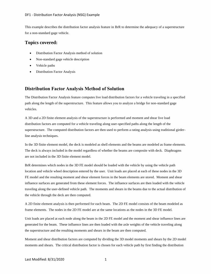
Non-standard gage vehicle description
Elevation View
12'-0"
Load/Axle Line
Load/Tire
Total Vehicle Weight
NSG Truck Load Data
40 kips
20 kips
88 kips
Front Axle
Load/Axle Line
Load/Tire
48 kips
12 kipsRear Axle
5'-0"
End View of Rear Axle
2'-6" 2'-6"
Vehicle CL
5'-0"
6'-3"
7'-6"
End View of Front Axle
Vehicle CL
3'-9"
7'-6"
The preceding non-standard gage vehicle can be entered in the BrR vehicle library as follows. Open the Library
Explorer in BrR.
DF1 - Distribution Factor Analysis (NSG) Example
Last Modified: 8/31/2020 3
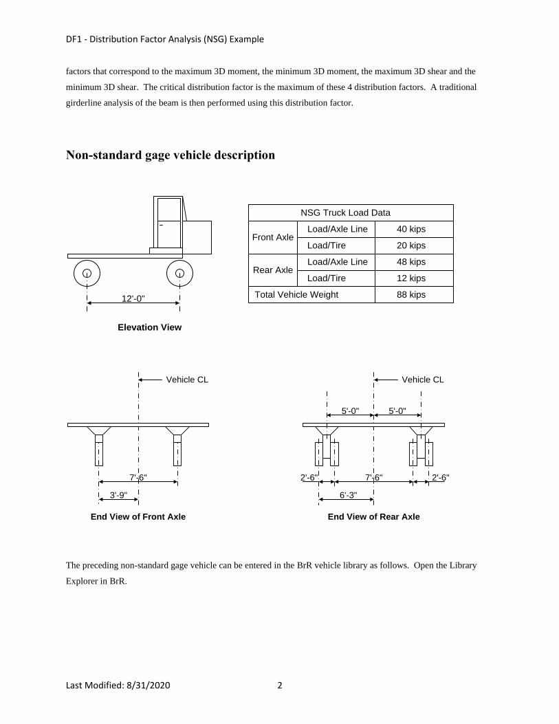
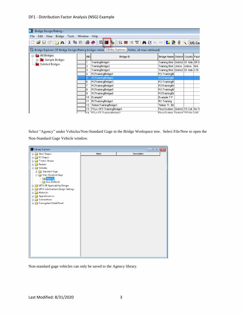
Select “Agency” under Vehicles/Non-Standard Gage in the Bridge Workspace tree. Select File/New to open the
Non-Standard Gage Vehicle window.
Non-standard gage vehicles can only be saved to the Agency library.
DF1 - Distribution Factor Analysis (NSG) Example
Last Modified: 8/31/2020 4
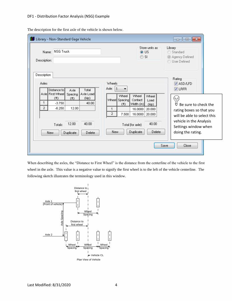
The description for the first axle of the vehicle is shown below.
When describing the axles, the “Distance to First Wheel” is the distance from the centerline of the vehicle to the first
wheel in the axle. This value is a negative value to signify the first wheel is to the left of the vehicle centerline. The
following sketch illustrates the terminology used in this window.
Distance to
first wheel
Plan View of Vehicle
Wheel
Spacing
Wheel
Spacing
Wheel
Spacing
Vehicle CL
Wheel
Spacing
Axle 2
Axle 1
Axle
Sp
acin
g
Distance to
first wheel
(Front of vehicle)
Be sure to check the
rating boxes so that you
will be able to select this
vehicle in the Analysis
Settings window when
doing the rating.
DF1 - Distribution Factor Analysis (NSG) Example
Last Modified: 8/31/2020 5
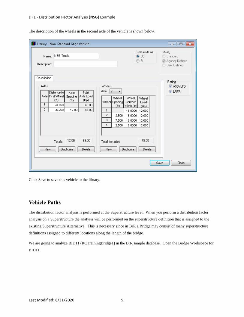
The description of the wheels in the second axle of the vehicle is shown below.
Click Save to save this vehicle to the library.
Vehicle Paths
The distribution factor analysis is performed at the Superstructure level. When you perform a distribution factor
analysis on a Superstructure the analysis will be performed on the superstructure definition that is assigned to the
existing Superstructure Alternative. This is necessary since in BrR a Bridge may consist of many superstructure
definitions assigned to different locations along the length of the bridge.
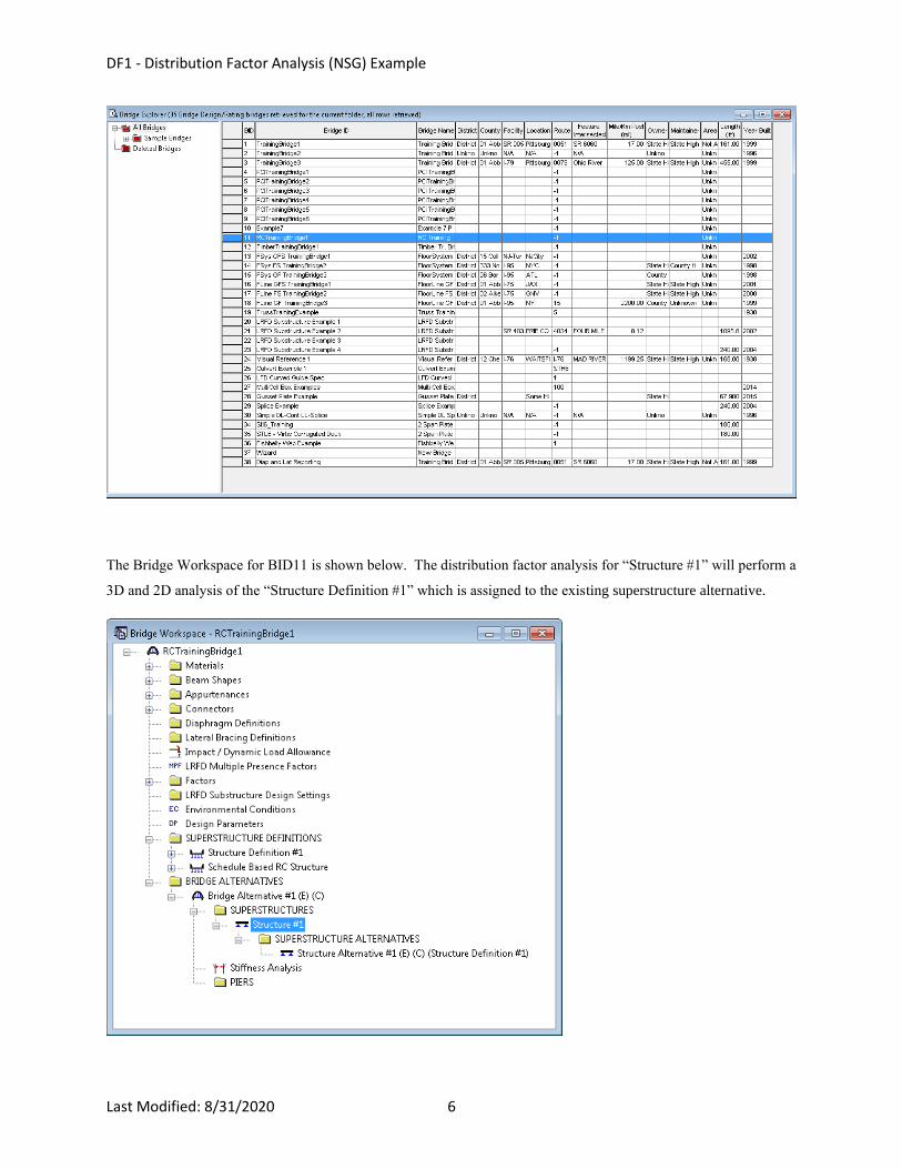
We are going to analyze BID11 (RCTrainingBridge1) in the BrR sample database. Open the Bridge Workspace for
BID11.
DF1 - Distribution Factor Analysis (NSG) Example
Last Modified: 8/31/2020 6
The Bridge Workspace for BID11 is shown below. The distribution factor analysis for “Structure #1” will perform a
3D and 2D analysis of the “Structure Definition #1” which is assigned to the existing superstructure alternative.
DF1 - Distribution Factor Analysis (NSG) Example
Last Modified: 8/31/2020 7
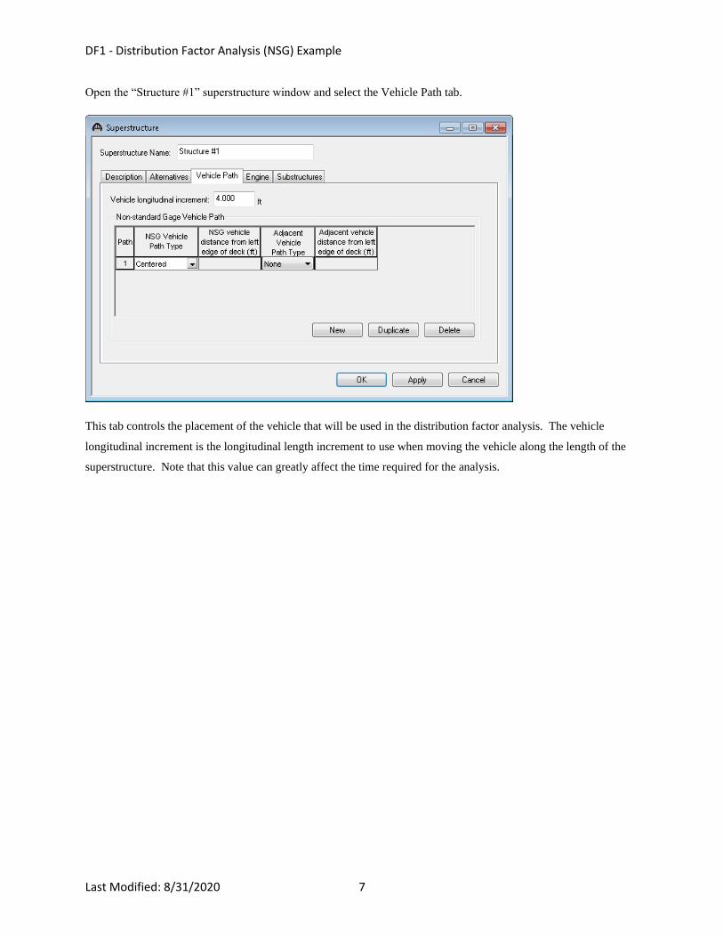
Open the “Structure #1” superstructure window and select the Vehicle Path tab.
This tab controls the placement of the vehicle that will be used in the distribution factor analysis. The vehicle
longitudinal increment is the longitudinal length increment to use when moving the vehicle along the length of the
superstructure. Note that this value can greatly affect the time required for the analysis.
DF1 - Distribution Factor Analysis (NSG) Example
Last Modified: 8/31/2020 8
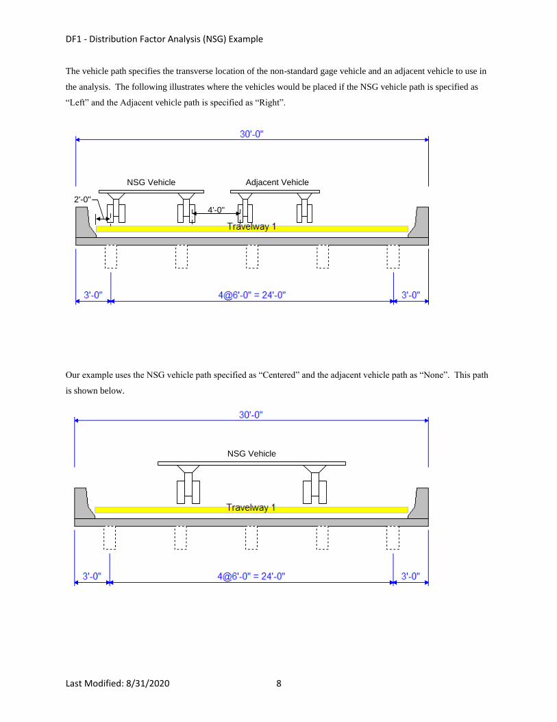
The vehicle path specifies the transverse location of the non-standard gage vehicle and an adjacent vehicle to use in
the analysis. The following illustrates where the vehicles would be placed if the NSG vehicle path is specified as
“Left” and the Adjacent vehicle path is specified as “Right”.
2'-0"
4'-0"
NSG Vehicle Adjacent Vehicle
Our example uses the NSG vehicle path specified as “Centered” and the adjacent vehicle path as “None”. This path
is shown below.
NSG Vehicle
DF1 - Distribution Factor Analysis (NSG) Example
Last Modified: 8/31/2020 9
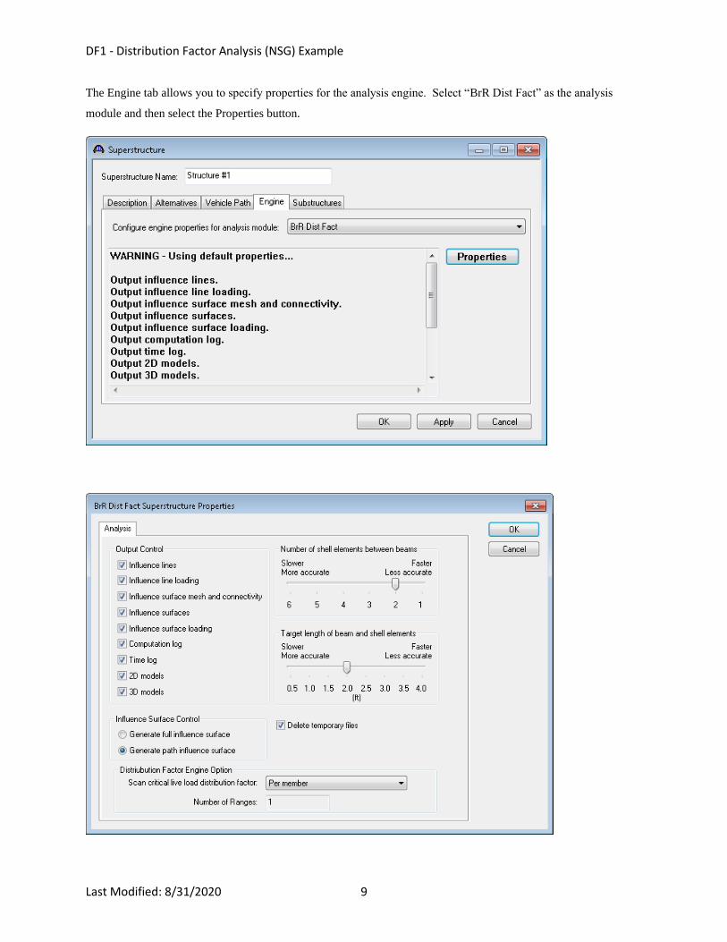
The Engine tab allows you to specify properties for the analysis engine. Select “BrR Dist Fact” as the analysis
module and then select the Properties button.
DF1 - Distribution Factor Analysis (NSG) Example
Last Modified: 8/31/2020 10
This window allows you to specify the level of output that you want from the analysis and allows you to control how
the FE models are created and loaded. The “Number of shell elements between beams” and “Target length of beam
and shell element” selections control the size of the elements in the model and also greatly influence the time
required for the analysis.
Click OK to close the BrR Dist Fact Superstructure Properties window and then click OK again to close the
Superstructure window.
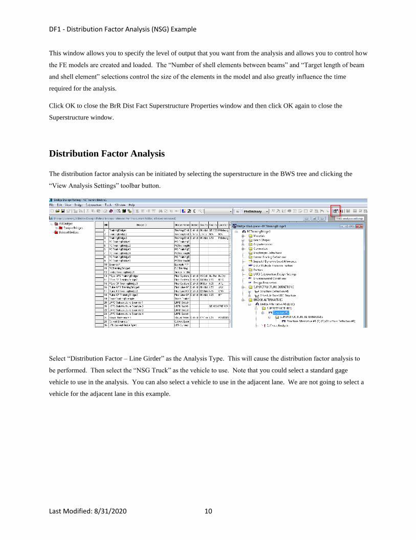
Distribution Factor Analysis
The distribution factor analysis can be initiated by selecting the superstructure in the BWS tree and clicking the
“View Analysis Settings” toolbar button.
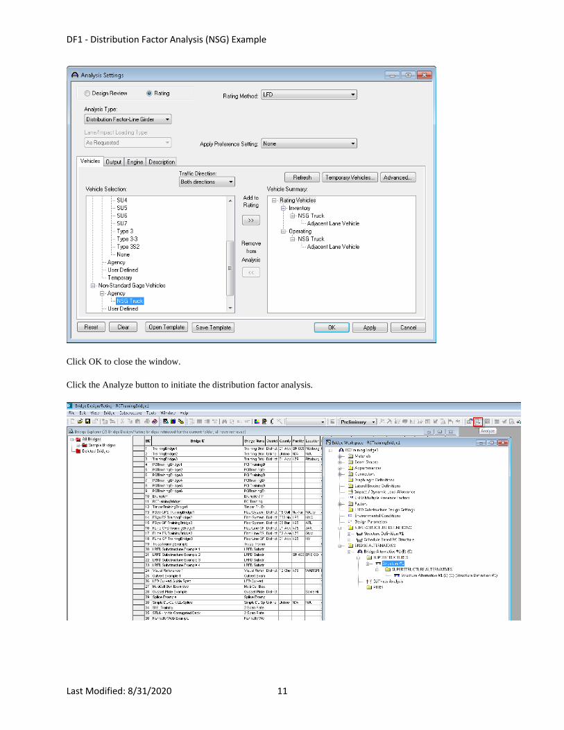
Select “Distribution Factor – Line Girder” as the Analysis Type. This will cause the distribution factor analysis to
be performed. Then select the “NSG Truck” as the vehicle to use. Note that you could select a standard gage
vehicle to use in the analysis. You can also select a vehicle to use in the adjacent lane. We are not going to select a
vehicle for the adjacent lane in this example.
DF1 - Distribution Factor Analysis (NSG) Example
Last Modified: 8/31/2020 11
Click OK to close the window.
Click the Analyze button to initiate the distribution factor analysis.
DF1 - Distribution Factor Analysis (NSG) Example
Last Modified: 8/31/2020 12
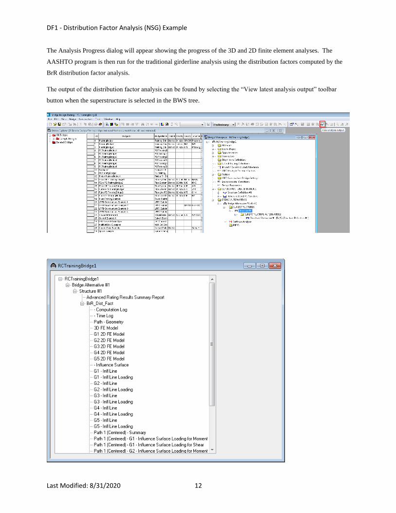
The Analysis Progress dialog will appear showing the progress of the 3D and 2D finite element analyses. The
AASHTO program is then run for the traditional girderline analysis using the distribution factors computed by the
BrR distribution factor analysis.
The output of the distribution factor analysis can be found by selecting the “View latest analysis output” toolbar
button when the superstructure is selected in the BWS tree.
DF1 - Distribution Factor Analysis (NSG) Example
Last Modified: 8/31/2020 13
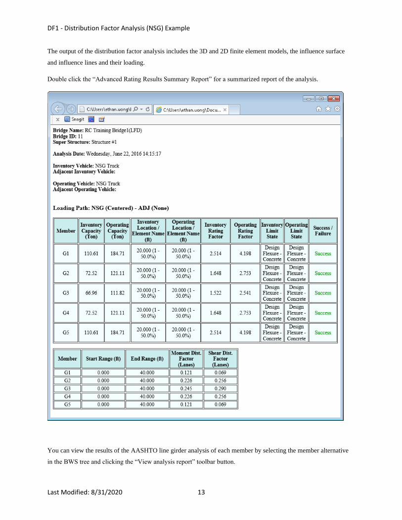
The output of the distribution factor analysis includes the 3D and 2D finite element models, the influence surface
and influence lines and their loading.
Double click the “Advanced Rating Results Summary Report” for a summarized report of the analysis.
You can view the results of the AASHTO line girder analysis of each member by selecting the member alternative
in the BWS tree and clicking the “View analysis report” toolbar button.


