Distributional preferences and the incidence of costs and benefits in climate change policy

Beilei Cai, Trudy Ann Cameron* Department of Economics, 435 PLC,

1285 University of Oregon, Eugene, OR 97403-1285

and

Geoffrey R. Gerdes Board of Governors of the Federal Reserve System,

Washington, DC, USA

November 12, 2009 * Correspondence (e-mail: cameron@uoregon.edu ) Acknowledgements: The data for this study were collected with funding from the National Science Foundation (SES-9818875). This research was supported in part by the endowment of the R.F. Mikesell Chair in Environmental and Resource Economics at the University of Oregon. We are grateful to Vilija Gulbinas for assistance with survey development and implementation at UCLA. We are also grateful for the very generous cooperation of 114 instructors at 92 different colleges and universities in the U.S. and Canada who announced our survey to their classes and encouraged participation, and to participants at the 2007 Heartland Environmental & Resource Economics Workshop (Ames, IA), the 2007 CU Environmental and Resource Economics Workshop (Vail, CO), and the 2008 EAERE conference (Gothenburg, Sweden). Dan Burghart and Ron Davies have also provided helpful suggestions. The opinions expressed in this paper are those of the authors and do not necessarily reflect the opinions of the Federal Reserve Board of Governors or its staff.

Distributional preferences and the incidence of costs and benefits in climate change policy

Abstract: We explore the relationship between willingness to pay (WTP) for climate change mitigation and distributional preferences, by which we mean individuals’ opinions about who should be responsible for climate change prevention and whether the share of climate change impacts borne by the poor is a cause for concern. We use 1770 responses to an online stated preference survey. The domestic costs in our survey’s policy choice scenarios are expressed as a set of randomized shares across four different payment vehicles, and the international cost shares are randomized across four groups of countries. We also elicit respondents’ perceptions of the likely regressivity of climate change impacts under a policy of business-as-usual. WTP is higher when larger cost shares are borne by parties deemed to bear a greater responsibility for mitigation, and when respondents believe (and care) that the impacts of climate change may be borne disproportionately by the world’s poor. That WTP for an environmental policy depends on the distributional consequences of the policy is an unsettling result: efficiency assessments are typically assumed to be separate from equity considerations in most benefit-cost analyses. Key words: climate change, distributional preferences, equity, regressivity, stated preference, payment vehicle, construct validity JEL: C35, C42, H41, Q51, Q54

I. Introduction The 2007 Nobel Peace Prize was awarded to the Intergovernmental Panel on Climate Change

(IPCC) and Albert Gore “for their efforts to build up and disseminate greater knowledge about

man-made climate change, and to lay the foundations for the measures that are needed to

counteract such change." According to the Nobel Committee, “[e]xtensive climate changes may

alter and threaten the living conditions of much of mankind. They may induce large-scale

migration and lead to greater competition for the earth's resources. Such changes will place

particularly heavy burdens on the world's most vulnerable countries. There may be increased

danger of violent conflicts and wars, within and between states.” In other words, climate policy

is relevant to world peace because of its distributional consequences. We might (a.) allow

climate change to proceed, via a policy of business-as-usual, and merely learn to adapt, or (b.)

embark upon more- or less- aggressive policies to limit climate change. Depending upon our

choices, the domestic and international distributions of net benefits are likely to be very different

and perhaps very unequal. This inequality has the potential to cause significant regional and/or

global strife. As Stern (2006) emphasizes in his landmark review of climate change for the U.K.

government, “Climate-related shocks have sparked violent conflict in the past, and conflict is a

serious risk in areas such as West Africa, the Nile Basin and Central Asia” (p. vii).1

The distribution of costs and benefits has been an important issue in climate negotiations as

well. Many different authors have considered the distribution of climate change impacts and

issues related to the problem of how to craft domestic policies and international agreements

concerning climate change mitigation which are sufficiently acceptable in terms of their

distributional consequences. Some examples include Azar and Sterner (1996), Stephan and

1Some reactions to the Stern Review include Nordhaus (2007) and Weitzman (2007), as well as a symposium in the Review

of Environmental Economics and Policy, including Mendelsohn (2008), Sterner and Persson (2008), Weyant (2008), and Dietz and Stern (2008), as well as further comments and rejoinders in subsequent issues.

2

Muller-Furstenberger (2004), Reibstein (2005), Thomas and Twyman (2005), Lange (2006),

Mendelsohn et al. (2006), Parks and Roberts (2006), Raymond (2006), and Anthoff et al. (2009).

In contrast to these types of studies, we investigate individual preferences for climate change

policies. Lange et al. (2007) survey a sample of individuals who are actually involved with

international climate policy, but we explore the preferences of ordinary non-experts. We

demonstrate that the distributional consequences of climate change policy—both in terms of the

domestic and international distributions of mitigation costs, and the regressivity of perceived

climate change impacts in the absence of mitigation—can have strongly significant effects on

individual willingness to pay for prevention for some people, although not for everyone.

Numerous other studies which have sought to value environmental public goods have

certainly included people’s attitudes about the importance of these public goods as determinants

of willingness to pay for their protection. To our knowledge, however, this is the first study of

willingness to pay (WTP) for climate change mitigation to undertake a comprehensive

assessment of the effects of heterogeneity in normative opinions about responsibility for

mitigation and concerns about the regressivity of climate change impacts. Different perceptions

about responsibility are very clearly relevant to how domestic and international policy-making

authorities might contemplate the implementation of future climate policies.

To address normative preferences over the distribution of costs and benefits in climate

change mitigation policies (including a policy of no action), we use a comprehensive online

survey of individuals concerning their personal climate policy preferences. At the core of this

survey, after an extensive preamble, is a so-called “stated preference” (SP) question concerning

some alternative policy options. The question is posed as a hypothetical referendum, and each

3

policy alternative is described in terms its likely costs and benefits.2 In the existing literature,

Flores and Strong (2007) note that benefit-cost analysis, especially when it employs stated

preference methods, cannot be done properly without careful attention to the question of who

will pay the costs. These authors note that “If researchers are eliciting values for public goods,

they need to make clear the costs to others.” Our survey does an unusually thorough job of

specifying how the costs of the different policy options will be borne.

The review by Stern (2006) points out that “Policies also have important differences in

their consequences for the distribution of costs across individuals, and their impact on public

finances” (p. xviii). Ours appears to be the first SP climate policy survey to randomize, across its

choice scenarios, both the domestic distribution of the initial incidence of mitigation costs, and

the international distribution of global mitigation costs across different country groups.3 We

also elicit from each respondent a subjective assessment of the extent to which the adverse

effects of climate change will be borne by the poorest 50% of the world’s population. This is

interpreted as an estimate of the expected regressivity of a business-as-usual policy, when

nothing is done to prevent climate change. This expected regressivity is reflected in the Stern

Review’s recognition that the “…impacts of climate change are not evenly distributed – the

poorest countries and people will suffer earliest and most.” (See Stern (2006), p. vii.)

Our analysis makes use of normative opinions, elicited from each individual survey

respondent, which allow us to control for certain types of preference heterogeneity that are

typically unobserved. Most stated preference surveys collect an array of observable

2 Stated preference studies of consumer demand have been used widely in the marketing literature, the transportation economics literature, the environmental economics literature, and increasingly in the health economics literature. Early examples were fraught with problems, but much has been learned over the last two decades in how to design these surveys to collect the most reliable information possible. Where actual revealed preference (RP) information is available, most economists still strongly prefer to rely on these actual choices as their data. In many cases, however, no appropriate RP information is available, and SP survey data represent the best possible alternative source of information about consumer demands.

3 In a review of existing SP studies, Schlapfer (2006) finds that very few such surveys employ payment mechanisms which are sophisticated enough to cover various payment vehicles with specific cost distributions.

4

sociodemographic characteristics for each respondent. If preferences are allowed to be

heterogeneous, these observable characteristics are sometimes used as shifters for the preference

parameters in stated choice models.4

It is much less common to seek to measure directly each individual’s attitudes with

respect to different attributes of the policy alternatives in a set of stated preference choice

scenarios. In our study, we ask each respondent about the extent to which they agree or disagree

with the responsibility of a range of different domestic and international groups to bear the costs

of climate change mitigation. We also enquire about the extent to which each individual

professes to be worried about the equity or fairness of likely climate change impacts. We argue

that these attitudes (or levels of concern) are some of the underlying latent factors that we would

typically attempt to proxy using observable sociodemographic characteristics. In this survey,

however, we have direct measures of these attitudes.

Our paper shows that the distributions of costs and benefits associated with climate

change policy are considered by some respondents to be relevant policy attributes in deciding

their willingness to pay (WTP) for that policy. The distributional consequences have greater

relevance to individuals who have explicitly agreed (or explicitly disagreed) with separate

statements concerning the degree of responsibility for mitigation costs that should belong to

those groups who are described as bearing larger shares of those costs under the policy scenario

in question. Additionally, WTP is enhanced when a respondent both believes that climate change

impacts will be regressive, and cares about this outcome.

4 As an alternative approach to preference heterogeneity, the researcher may allow each preference parameter

to vary randomly. A distributional family is specified for each preference parameter and the researcher estimates both the expected value and the dispersion of each parameter (and sometimes the covariances among parameters) across the sample. More rarely, preference parameters may vary both systematically with observable characteristics, and randomly, in the same model.

5

We also demonstrate considerable systematic heterogeneity in WTP according to a

number of sociodemographic and ideological variables. It is striking that for a number of

different groups, there is little evidence that WTP exceeds zero unless the variables which

capture distributional attitudes are brought into play. However, under the right mix of policy

attributes (domestic and international cost distributions), expectations about climate change

impacts, sociodemographic characteristics, and attitudes (distributional preferences), predicted

WTP can be dramatically higher. Disagreements about the urgency of climate change mitigation

policy undoubtedly stem from this heterogeneity in beliefs and attitudes, as well as from

differences in the likely incidence of the costs and benefits of every possible policy, including the

status quo.

Finally, our evidence that WTP for climate change mitigation policies depends critically

upon respondents’ stated distributional preferences is an unsettling result from the perspective of

benefit-cost analysis of public programs and regulations. Economists commonly approach

welfare analysis by assuming that efficiency considerations can be divorced from equity

concerns. Flores (2002), though, raises the question of whether purely selfish values for public

goods exist, in practice. Our empirical findings respond to Flores’ question. “Purely selfish

values” for an environmental public good could presumably be derived independent of any

information about how much others might benefit from the policy or how much they would be

required to pay for it. Based on our results, we argue that the usual WTP estimates employed as

benefits measures in the types of benefit-cost analyses that address efficiency questions should

be approached with caution. We contend that individual WTP often cannot be derived without

reference to the distributional consequences (be they explicit or imputed) of the proposed policy

or regulation, controlling for each individual’s attitudes about these distributional consequences.

Such normative concerns probably apply much more broadly than to just this climate policy

6

study. We argue that issues such as those explored in this study should be on the table—from the

design stages through the final analysis—in most economic assessments of public policies and

proposed regulations.

The research described in this paper has connections to a number of persistent themes in the

literature on the valuation of non-market public goods. First, it is well-known that the “payment

vehicle” (i.e. who will pay for a policy, and how) can matter very much in studies designed to

determine WTP for a non-market public good. This is typically because different payment

vehicles imply different initial incidence for policy costs and therefore different distributional

impacts for a policy. Payment vehicle effects also reflect perceptions about opportunities for

free-riding, where subjects may prefer a payment vehicle that imposes a greater share of the costs

of the policy on someone else. In SP studies, the designated payment vehicle conveys an implicit

incidence for the costs of the policy and can thus it be a crucial determinant of willingness to pay

(WTP) for improvements in non-market environmental goods. This undesirable sensitivity

reveals that respondents, on average, prefer some types of payment vehicles (i.e. some types of

distributional consequences) to others.5,6

Another vein in the literature concerns the “polluter-pays” principle (PPP) and related

notions of clean-up responsibility that have been examined in previous studies. Johnson (2006)

suggests that individuals are inclined to pay more when the cost share paid by polluters increases.

In the present study, we are specifically interested in individuals’ preferences over the

5 An assortment of payment vehicle issues are addressed in de Blaeij et al. (2003), Rollins (1997), Bergstrom et al. (2004), Morrison et al. (2000), and Florax et al. (2005). The literature has also touched on other questions about the details of how a public good would be provided. Stevens et al. (1997) find that respondents’ valuations of a good can be quite sensitive to whether periodic or lump sum payment schedules are employed. Champ et al. (2002) determine that payment mechanisms with differing incentive structures give rise to different implied values.

6 In a related vein of the empirical literature, it has been noted that respondents’ preferences over the distributional consequences implied by payment vehicles can trigger so-called “protest votes,” and the researcher’s choice of payment vehicle can thus play an important role in managing the odds of such protest votes. Jorgensen and Syme (2000) note that voters may object to only one aspect of the SP survey, such as the selected payment vehicle and its coverage. Morrison, Blamey et al. (2000) find that incorporating respondents’ attitudes toward the selected payment vehicle may reduce the bias resulting from differences in the coverage of payment vehicles.

7

distribution of costs among various categories of payers (domestically, via their exposures to

different types of payment vehicles). In contrast to earlier studies, however, the choice is not

whether the costs will be paid just by polluters, or by the general population. Instead, the general

population is collectively required to pay all the costs, but policies differ in terms of which

segments of society will bear what share of these costs. Individuals may play a variety of roles in

society, such as taxpayers, consumers, energy users, and industry investors. Furthermore,

everyone is a polluter, in some capacity, when it comes to climate change. Realistically, the

initial incidence of domestic policy costs is likely to be felt via a variety of payment vehicles

simultaneously (including income tax increases, consumer price increases, energy tax increases,

and decreases in investment returns). We randomly assign a stated cost share for all four of these

domestic payment vehicles, and examine how people’s utility from a proposed policy differs

when the cost share assigned to each payment vehicle varies. Stated international shares of

global mitigation costs are also randomly assigned for the same research purpose. This aspect of

the survey design allows us to examine the influence on policy choices of respondents’

preferences across payment vehicles (domestically) and different groups of countries

(internationally).

SP methods are typically afforded much greater scrutiny than revealed preference (RP)

methods as a tool for benefit-cost analysis.7 SP researchers thus endeavor to verify the

“theoretical construct validity” of SP estimates in variety of ways. The models examined in this

paper can also be interpreted as tests of the theoretical construct validity of respondents’ WTP for

climate change mitigation programs.8 WTP and planned behavioral changes have been shown to

7 A standard citation for early criticism of SP methods is Diamond and Hausman (1994). An early assessment

by an independent Blue Ribbon Panel is reported in Arrow et al. (1993). 8 “Theoretical” construct validity generally refers to the correlation of implied individual WTP amounts with

other objective or subjective factors that logic suggests should be systematically related to the magnitude of WTP. So-called “convergent” construct validity is sometimes also assessed (e.g. by assessing the correspondence between

8

depend on beliefs and attitudes about environmental public goods in many contexts, but in this

paper, we show that that the stated choices also bear plausible relationships to respondents’

preferences over the mix of payment vehicles (i.e. the distributional consequences in terms of

climate change mitigation policy costs) as well as their concerns about the potential regressivity

of the status quo option. These identified regularities should encourage future researchers, in

many different welfare assessment contexts, to elicit and use respondents’ normative opinions

about responsibility for policy costs and the potential regressivity of different policy options.

At this point, we need to be very clear about the innovations offered by this research.

Competent benefit-cost analysts have always been concerned with the distributional

consequences of alternative policies.9 Typically, individual net benefits are determined, then the

policy-maker considers the distribution of these individual net benefits across different segments

of the population, as in the type of tableau recommended by Krutilla (2005).10 Overall social net

benefits can only be determined after a set of distributional weights has been selected, although

these weights often default to equality. In contrast, our work emphasizes that distributional

considerations cannot be postponed to a second step that is subsequent to the calculation of

individual net benefits. Instead, individual net benefits often cannot be determined without

specific reference to the distributional consequences of the proposed policy, both in terms of

benefits and in terms of costs.

averting costs and WTP estimates, as in Laughland et al. (1996). Alternately it is sometimes possible to compare WTP inferences from respondents’ expressed voting preference and estimated WTP, as in Berrens et al. (1998), and between WTP estimates obtained from different elicitation methods (see Whitehead et al. (1998)).

9 Atkinson et al. (2000) and Turner (2005) discuss the practice of benefit-cost analysis, the use of equal weights or alternative social welfare functions, and other considerations with respect to environmental equity.

10 Krutilla (2005) proposed a Kaldor-Hicks tableau for assessment of the distributional consequences of a project. This is a matrix where rows give the types of benefits, costs, and financial transfers, and the columns disaggregate these effects by stakeholder group. This fuller disclosure of the distribution of benefits, costs, and transfers makes it easier for policy-makers to appreciate the net benefits for different groups and, presumably, to employ subjective discretionary weights in the process of making a decision.

9

II. Available Data: The online climate change survey The sample used here is drawn from a population consisting primarily of college students

who were surveyed during 2001. Respondents were recruited by 114 different instructors from

classes at 92 different colleges and universities throughout the U.S. and Canada. Our dataset

consists of 1770 responses to a comprehensive online survey of climate change. This

multi-campus analog to a conventional classroom survey (http://globalpolicysurvey.ucla.edu )

uses a remotely administered Web-based questionnaire.11,12

A. Predicted impacts of climate change

Many scientists now believe that climate change has the potential to pose major threats to

agriculture, weather, human health, and ecosystems.13 In our survey, we elicited respondents’

subjective concerns about climate change impacts across five broad categories. We asked: “How

worried are you about the vulnerability to climate change of each of the following?” The

categories of impacts were described as “Agriculture, Water,” “Ecosystems,” “Human health,”

“Oceans, Weather,” and “Equity, Fairness.” Respondents’ levels of concern regarding each

11 The core portions of this survey are very similar to those of a related general-population mail survey

reported in Lee and Cameron (2008). The randomizations in that survey were less extensive, since the mail survey format is more limiting than the online medium employed for this study. To demonstrate the presence of preferences over the distributional consequences of alternative policies, the more homogeneous student sample actually seems to make it easier for us to detect systematic effects. It is less necessary to control for variables such as age, education, employment status, marital status, etc., that might confound our ability to detect significant distributional preferences in a sample of fewer than 2000 respondents.

12 Berrens et al. (2003) and Berrens et al. (2004) report upon the findings from another extensive online climate survey. They employ a split-sample design where respondents were given either “basic information” or “enhanced information” about global climate change and the Kyoto Protocol, and their survey uses “increased energy and gasoline prices,” alone, as the payment vehicle. They also use an 11-level scale which measures whether the respondent believes that the Kyoto Protocol is fair, and respondents who perceived greater fairness had higher WTP values. Our survey goes into considerably greater detail on the fairness dimension. Our different climate policies vary in their level of cost to the individual and the domestic and international distribution of their costs, and heterogeneous measures of the size and distribution of climate change impacts (benefits of mitigation) are subjectively elicited. We elicit attitudes that correspond to respondent’s perceptions of fairness on all of these dimensions.

13 For example, see Bosello et al. (2006), Kelly et al. (2005), Kinnell et al. (2002), and Kurukulasuriya et al. (2006).

10

category of impacts can be described as one of the alternatives “not worried,” “somewhat

worried,” “very worried,” and “don’t know.”14

We also elicited respondents’ subjective expected ratings of anticipated climate change

impacts: “Worldwide, how do you think climate change will affect each of the following, by 30

years from now, if a policy of ‘Business-as-Usual’ is followed?” 15 Respondents were invited to

rate climate change impacts (as either single values or intervals) on a simple nine-point

scale—ranging from -4 for extremely negative impacts, to +4 for extremely positive impacts.16

B. Attitudes

Respondents were specifically asked to indicate their attitudes about the extent to which

responsibility for the costs of climate change mitigation should be borne by various payers.17

Six classes of domestic payers are proposed, including individual tax-payers, consumers, energy

users, industry (investors), energy producers, and “government.” Seven types of international

payer groups were also proposed, including industrialized countries, the countries of the former

Soviet Union, densely populated developing countries like India and China, the United States

and its major trading partners, developing countries that are beginning to pollute heavily, the

14 We provide an Online Appendix containing selected examples of screens from our randomized online

survey. Online Appendix Figure A.1 shows one example of how respondents were invited to rate their degree of worry about different impacts. The Equity & Fairness impact was always listed last, but the other four types of impacts appeared in random order across respondents (although in a consistent order within each survey instrument). Degree of worry and WTP has been explored in other contexts in Hanley et al. (2001) and Schade et al. (2002).

15 Focus groups made it clear that it would be impossible to elicit complete anticipated time profiles of future climate change impacts, so we opted to have them focus on just one future date, far enough out that detectible effects might be anticipated, but not so far as to lie beyond the life expectancy of someone currently fifty years of age.

16 Online Appendix Figure A.2 shows one example of the elicitation of anticipated climate change impacts. We initially use the point values or interval midpoints for these ratings as an approximately continuous measure of anticipated climate change impacts on each dimension. [A complete distribution of these detailed point values or interval midpoints is presented in Online Appendix Table B.1.]

17 An example of this survey screen appears in Online Appendix Figure A.3. In this variant, five answer options were available for each question. The design of the questionnaire incorporates an unusually wide array of dynamically generated randomized elicitation formats that permit assessment of the sensitivity of choices to different elicitation strategies. On the surface, these different elicitation formats may appear to be arbitrary and inconsequential, but empirically, they may have systematic effects upon choices (e.g. DeShazo and Fermo (2002), Hensher (2006)). In this paper, we merely control for such differences where necessary, rather than make their effects the focus of the analysis.

11

smaller developing countries, and “countries in proportion to their contribution to the problem.”

In the most-extensive elicitation format, respondents’ attitudes could be one of the following:

“agree strongly,” “agree,” “neutral,” “disagree,” or “disagree strongly.”

Attitudes about who should bear the costs of climate change are certainly intertwined with

the mix of selfish and other-regarding preferences that characterizes each respondent. Someone

who has an income low enough that they pay relatively little income tax may be more favorably

inclined towards climate policies where income taxes fund a greater share of the initial costs of

mitigation. Someone with a substantial portfolio of investments may be less in favor of a policy

where the initial impact is felt more in the form of lower investment returns.

C. Climate policy choices

In split samples, either two or three policy alternatives were proposed. In the two-alternative

case, these included “Maximum climate change prevention” which we label as Complete

Mitigation (CM) and Business-as-Usual (BAU).18 CM is when the respondent’s anticipated

climate change impacts are essentially prevented, keeping the climate much as it is today.

However substantial costs would be incurred to achieve this goal. Under a BAU policy, however,

the respondents’ anticipated climate change impacts will be realized, perhaps with implicit

adaptation expenses, but no additional climate change mitigation costs will be incurred.

Respondents who were presented with three-alternative choice sets also saw an intermediate

option called “Partial Mitigation” (PM), where the BAU impacts are scaled back

18 The survey itself uses the term “prevention” rather than “mitigation,” since focus groups showed that not

everyone was familiar with the mitigation term. In our empirical model, we include a shared increment to indirect utility for any alternative involving a departure from the status quo, plus a second increment for the partial mitigation option, when it is offered. The marginal utility associated with these indicator variables helps to keep some additional unobserved heterogeneity, across alternatives, out of the error term.

12

non-proportionately, but not eliminated, and the cost of the policy is randomly lower than for

CM.19

Under PM and CM, the overall domestic prevention cost is randomized in terms of the

expected costs that households will have to pay, subject to the constraint that the cost for PM is

always less than that for CM. We convey to individuals that the initial incidence of climate

change mitigation costs will be felt in a variety of different ways, according to how the policy is

implemented. Domestic costs are experienced through four different payment vehicles: decreases

in investment returns, and increases in consumer prices, income taxes, and energy taxes. The cost

shares experienced via each payment vehicle are randomized in 5% increments over the range

from 10% to 70%, subject to the constraint that they sum to 100%.

The international costs of climate change mitigation, explained separately to respondents,

are shared across four subsets of the world’s countries: “US and Japan,” “other industrialized

countries,” “India and China,” and “other developing countries.” International costs for other

countries are not borne by domestic households. Domestic costs are thus assumed to be viewed

by respondents as one component of a more-or-less coordinated international climate policy.

Each group of countries needs to bear a certain percentage of the overall global cost.

International cost shares across country groups also range from 10% to 70% and are completely

randomized.20

D. Concern about climate change

Individuals’ stated levels of concern about climate change may play an important role in

their willingness to incur the costs of prevention. Respondents were asked to rate their personal

priority levels for eleven randomly ordered issues which are likely to be of global concern. These

19 Online Appendix Figure A.4 gives one example of the survey’s dynamically generated two-alternative

choice scenario and Figure A.5 shows one three-alternative choice scenario. 20 Li et al. (2004) address the international sharing of climate change mitigation costs in the Kyoto Protocol.

13

issues included preventing climate change, improving food safety, preventing wars, reducing

poverty and hunger, etc.21 In the most-extensive elicitation format, the priority levels the

individual could assign included “very high priority,” “high priority,” “moderate priority,” “low

priority,” “not a priority at all” and “not sure.” Collected prior to the individuals’ stated

preferences over climate policy, this information reveals respondents’ likely baseline level of

concern about climate change in the context of a wider list of other problems faced by society.22

The sociodemographic questions at the very end of the survey also asked whether the respondent

belonged to any environmental groups.

III. Estimating Specification

Suppose respondent i sees all three policy alternatives: CM, PM, and BAU.23 This

respondent’s anticipated indirect utility under policy j (where j= CM, PM, or BAU) can be

described generically as

* (( ), , , )j j j j ji i i i i iV Y C B DC IC− (1)

where ( )j

i iY C− denotes the choice-specific net income (after any mitigation costs) that the

respondent’s household will enjoy under policy j , and jiB denotes the choice-specific

21 One example of this screen is contained in Online Appendix Figure A.6. 22 Other aspects of our online climate survey have been used in several other analyses. Cameron and Gerdes

(2005) look exclusively at the survey module designed to elicit individual-specific estimates of financial discount rates using intertemporal choices. Cameron and Gerdes (2006) combine the intertemporal financial choice question with a question about choices among risky and risk-free investments over a long time horizon, to explore the ability of estimated individual discount rate parameters and estimated individual risk aversion parameters to shift climate change preferences in an otherwise highly simplified model. Burghart et al. (2007) explore a survey module concerning willingness to divert a hypothetical tax credit into research in air conditioner technology, treated as an adaptation to climate change. Related work based on much simpler pretest versions of the survey, and a much smaller single-campus sample, has been published as Cameron (2005) and Cameron (2005).

23 Individuals who selected the “would not vote” option are excluded from our analysis. A more thorough analysis, designed to assess WTP for climate change mitigation in a more-representative sample (as opposed to the potential impact of the mix of payment vehicles) would require a more-complex econometric specification to accommodate this additional type of “response” to the choice question.

14

subjective expected benefits (equal to avoided climate change impacts). We assume that indirect

utility is increasing in both net income and climate change mitigation benefits.

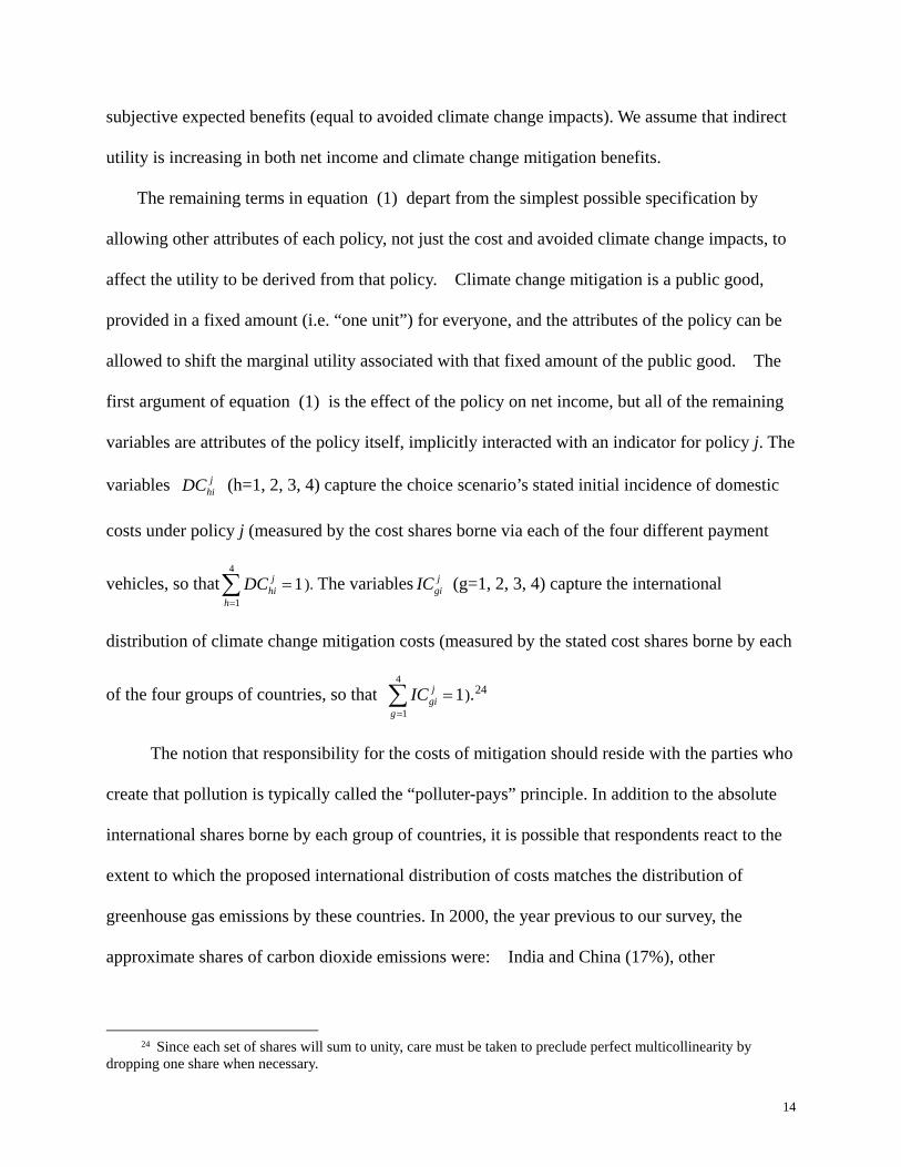
The remaining terms in equation (1) depart from the simplest possible specification by

allowing other attributes of each policy, not just the cost and avoided climate change impacts, to

affect the utility to be derived from that policy. Climate change mitigation is a public good,

provided in a fixed amount (i.e. “one unit”) for everyone, and the attributes of the policy can be

allowed to shift the marginal utility associated with that fixed amount of the public good. The

first argument of equation (1) is the effect of the policy on net income, but all of the remaining

variables are attributes of the policy itself, implicitly interacted with an indicator for policy j. The

variables jhiDC (h=1, 2, 3, 4) capture the choice scenario’s stated initial incidence of domestic

costs under policy j (measured by the cost shares borne via each of the four different payment

vehicles, so that4

11j

hih

DC=

=∑ ). The variables jgiIC (g=1, 2, 3, 4) capture the international

distribution of climate change mitigation costs (measured by the stated cost shares borne by each

of the four groups of countries, so that 4

11j

gig

IC=

=∑ ).24

The notion that responsibility for the costs of mitigation should reside with the parties who

create that pollution is typically called the “polluter-pays” principle. In addition to the absolute

international shares borne by each group of countries, it is possible that respondents react to the

extent to which the proposed international distribution of costs matches the distribution of

greenhouse gas emissions by these countries. In 2000, the year previous to our survey, the

approximate shares of carbon dioxide emissions were: India and China (17%), other

24 Since each set of shares will sum to unity, care must be taken to preclude perfect multicollinearity by

dropping one share when necessary.

15

developing countries (30%), US and Japan (31%), other industrialized countries (22%).25 We

require an index that measures the extent of the departure of a particular international cost share

distribution from this international distribution of emissions. One candidate measure can be

constructed using a formula analogous to that for a 2χ test statistic for differences in proportions.

Let gPP be the share of costs for country group g if costs were apportioned on the basis of

“polluter-pays.” Let jgiIC be the cost share borne by country group g under policy j

proposed in the choice scenario offered to individual i. We use the formula

( )4 2

1

jgi g g

gIC PP PP

=

− ∑ (2)

to summarize the extent of departure from “polluter-pays” for the international distribution of

climate policy costs. This index has a value of zero if the international distribution of costs

matches “polluter-pays.” As the departure from this distribution increases, this index will take on

larger and larger values. The expression in equation (2) becomes an additional attribute for each

policy, with an associated marginal utility. If respondents feel that adherence to the polluter-pays

principle is desirable, utility from a policy will decline as this index gets larger.26

The policy preference question presented to respondents is either a two-way or a three-way

choice, so a utility-theoretic discrete choice econometric specification is appropriate. Hence, we

use a conditional logit model, in combination with respondents’ stated climate policy preference,

to estimate the parameters of a specific version of the indirect utility function in (1). We partition

this indirect utility into a systematic portion and an unobservable (to the researcher) component:

* j j ji i iV V ε= + . We model the systematic portion of utility as a linear-in-parameters function of

25 Based on information available at http://unstats.un.org/unsd/ . Respondents were not given this

information in the survey. 26 We have considered alternative specifications which use the mean absolute deviation instead. The results

are qualitiatively the same.

16

the respondent’s anticipated circumstances under each policy alternative. Under CM, the

individual will bear costs CMiC and enjoy avoided climate change impacts (benefits) CM

iB , but

will also experience the stated domestic and international cost distributions associated with this

policy:

4 6 4 7*

0 01 1 1 1

24

0 10 111

2

( )

( )

( ) 1( )

CM CM CM CMi i i h hm mi hi g gn ni gi

h m g n

CMgi g B CM

p p pi i bi ig g

A CMi i

V Y C att DC att IC

IC PPatt Z att B

PP

Z Any Program

α θ θ θ θ

θ θ β β

β

= = = =

=

= − + + + +

− + + + +

+ +

∑ ∑ ∑ ∑

∑

( ) 1( )P CM CMi i iZ Partial Mitigationγ ε+

(3)

The miatt variables measure respondents’ attitudes concerning the responsibility for each of an

expanded list of m = 1,…6 categories of domestic payers. The niatt variables are analogous, but

they instead record respondents’ attitudes concerning the responsibility over each of an expanded

list of n = 1, 2, 3…6 international country groups. The variable piatt is a single variable, for the

7th opinion about international shares, namely whether countries should be held responsible “in

proportion to their contribution to the problem.”

The respondent’s individual subjective benefits of CM, CMiB , consist of the climate change

impacts which would be avoided if CM is pursued—namely, the difference between the (roughly)

zero impact under the policy, and the BAU impacts without it: (0 )CM BAUi iB IMPACTS= − . Prior

to the policy choice scenario, the potential BAU impacts have been rated by each respondent.

One expects that utility, and hence willingness to pay for climate change mitigation, should be

higher when greater negative impacts are expected in the absence of the policy. Thus we use the

negative of our measures of impact severity under BAU as our measure of the policy benefits.

Note that the marginal utility of explicit benefits, jiB , is allowed to vary across individuals

17

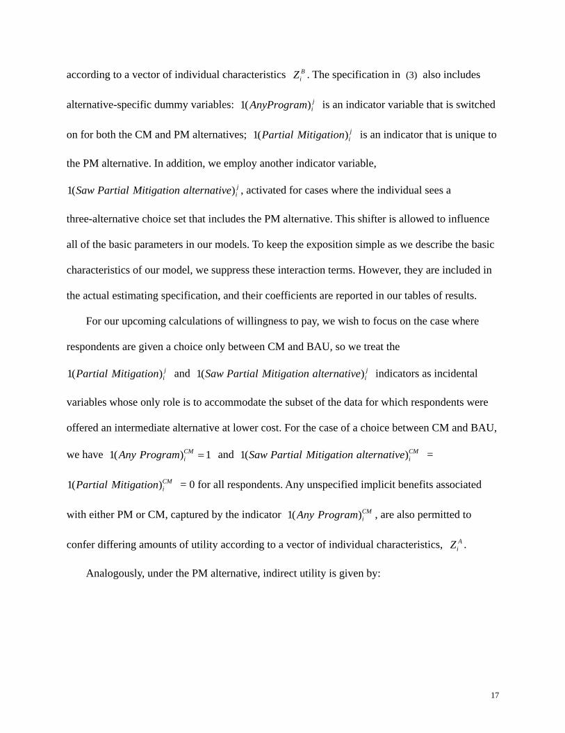
according to a vector of individual characteristics BiZ . The specification in (3) also includes

alternative-specific dummy variables: 1( ) jiAnyProgram is an indicator variable that is switched

on for both the CM and PM alternatives; 1( ) jiPartial Mitigation is an indicator that is unique to

the PM alternative. In addition, we employ another indicator variable,

1( ) jiSaw Partial Mitigation alternative , activated for cases where the individual sees a

three-alternative choice set that includes the PM alternative. This shifter is allowed to influence

all of the basic parameters in our models. To keep the exposition simple as we describe the basic

characteristics of our model, we suppress these interaction terms. However, they are included in

the actual estimating specification, and their coefficients are reported in our tables of results.

For our upcoming calculations of willingness to pay, we wish to focus on the case where

respondents are given a choice only between CM and BAU, so we treat the

1( ) jiPartial Mitigation and 1( ) j

iSaw Partial Mitigation alternative indicators as incidental

variables whose only role is to accommodate the subset of the data for which respondents were

offered an intermediate alternative at lower cost. For the case of a choice between CM and BAU,

we have 1( ) 1CMiAny Program = and 1( )CM

iSaw Partial Mitigation alternative =

1( )CMiPartial Mitigation = 0 for all respondents. Any unspecified implicit benefits associated

with either PM or CM, captured by the indicator 1( )CMiAny Program , are also permitted to

confer differing amounts of utility according to a vector of individual characteristics, AiZ .

Analogously, under the PM alternative, indirect utility is given by:

18

4 6 4 7*

0 01 1 1 1

24

0 10 111

2

( )

( )

( ) 1( )

PM PM PM PMi i i h hm mi hi g gn ni gi

h m g n

PMgi g B PM

p p pi i bi ig g

A PMi i

V Y C att DC att IC

IC PPatt Z att B

PP

Z Any Program

α θ θ θ θ

θ θ β β

β

= = = =

=

= − + + + +

− + + + +

+ +

∑ ∑ ∑ ∑

∑

( ) 1( )P PM PMi i iZ Partial Mitigationγ ε+

(4)

The PM alternative, when offered, is characterized by different costs and different cost

distributions, although the attitudes ( miatt and niatt ) which are allowed to shift the marginal

utilities on the cost shares will be assumed to be the same.

The benefits from PM will be less since the full climate change impacts that the individual

expects, under a policy of BAU, are only partially avoided. Thus the benefits under PM, PMiB ,

consist of a randomly assigned reduction (rather than an elimination) of the respondent’s

expected climate change impacts under BAU.27

Finally, under the status quo alternative (BAU), there are no mitigation costs. Thus, there are

no concerns about the distribution of these costs, either domestically or internationally. So

0BAUiC = , which means that the cost shares (implicitly interacted with a dummy variable for the

presence of mitigation costs) are zero. Likewise, there are no benefits (i.e. no “impact

reductions”) so 0BAUiB = for the explicit benefits. Only the net income term remains relevant,

so that

* ( )BAU BAUi i iV Yα ε= + (5)

For random utility models (RUMs), it is customary to designate a numeraire alternative

(here, the BAU alternative). Indirect utility-differences for each alternative, relative to this

27 As our benefits measure, we use the difference between the smaller (negative) impacts under PM and the

larger (negative) impacts under BAU: ( )PM PM BAUi i iB IMPACTS IMPACTS= − . Since the impacts under BAU will

be greater, the resulting measure will be a positive amount of “impact reduction.”

19

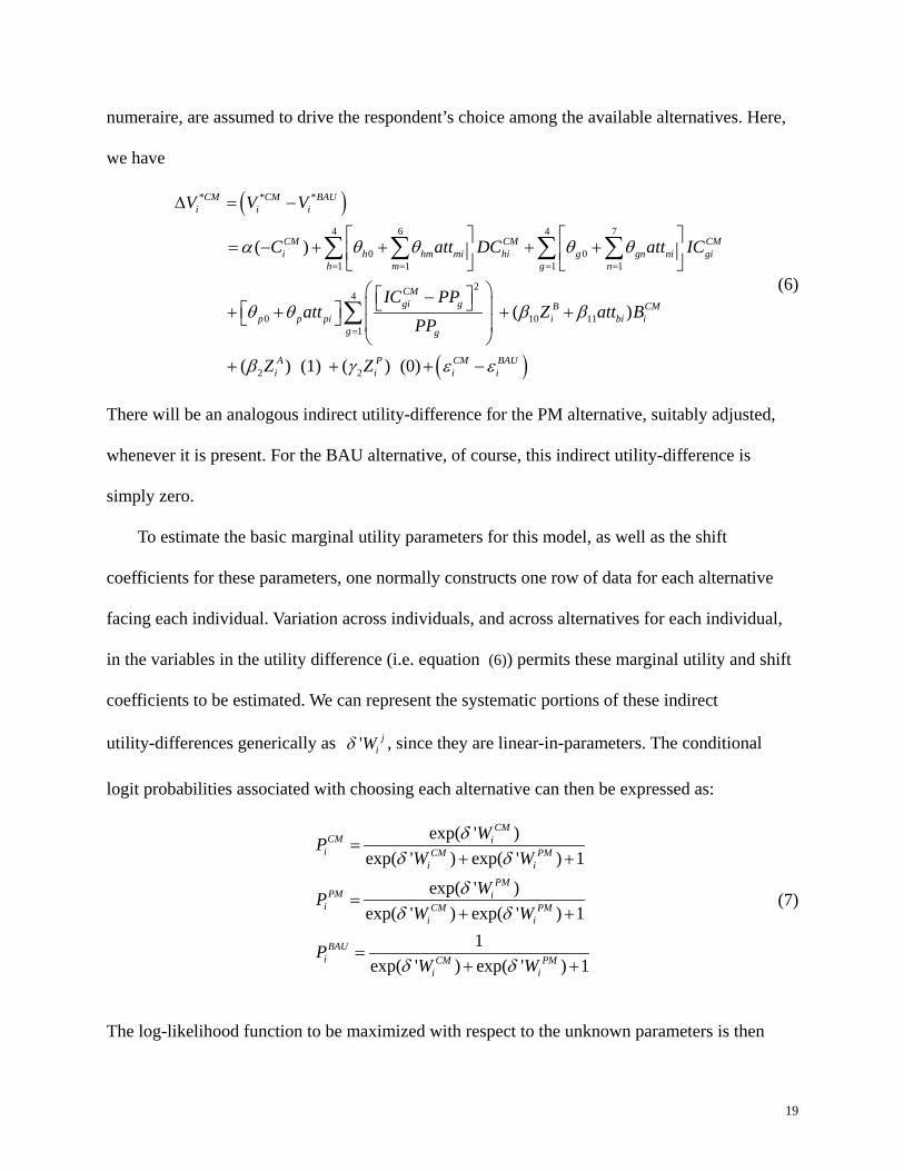
numeraire, are assumed to drive the respondent’s choice among the available alternatives. Here,

we have

( )* * *

4 6 4 7

0 01 1 1 1

24

0 10 111

( )

( )

CM CM BAUi i i

CM CM CMi h hm mi hi g gn ni gi

h m g n

CMgi g B CM

p p pi i bi ig g

V V V

C att DC att IC

IC PPatt Z att B

PP

α θ θ θ θ

θ θ β β

= = = =

=

∆ = −

= − + + + +

− + + + +

∑ ∑ ∑ ∑

∑

( )2 2 ( ) (1) ( ) (0)A P CM BAUi i i iZ Zβ γ ε ε+ + + −

(6)

There will be an analogous indirect utility-difference for the PM alternative, suitably adjusted,

whenever it is present. For the BAU alternative, of course, this indirect utility-difference is

simply zero.

To estimate the basic marginal utility parameters for this model, as well as the shift

coefficients for these parameters, one normally constructs one row of data for each alternative

facing each individual. Variation across individuals, and across alternatives for each individual,

in the variables in the utility difference (i.e. equation (6)) permits these marginal utility and shift

coefficients to be estimated. We can represent the systematic portions of these indirect

utility-differences generically as ' jiWδ , since they are linear-in-parameters. The conditional

logit probabilities associated with choosing each alternative can then be expressed as:

exp( ' )exp( ' ) exp( ' ) 1

exp( ' )exp( ' ) exp( ' ) 1

1exp( ' ) exp( ' ) 1

CMCM i

i CM PMi i

PMPM i

i CM PMi i

BAUi CM PM

i i

WPW W

WPW W

PW W

δδ δ

δδ δ

δ δ

=+ +

=+ +

=+ +

(7)

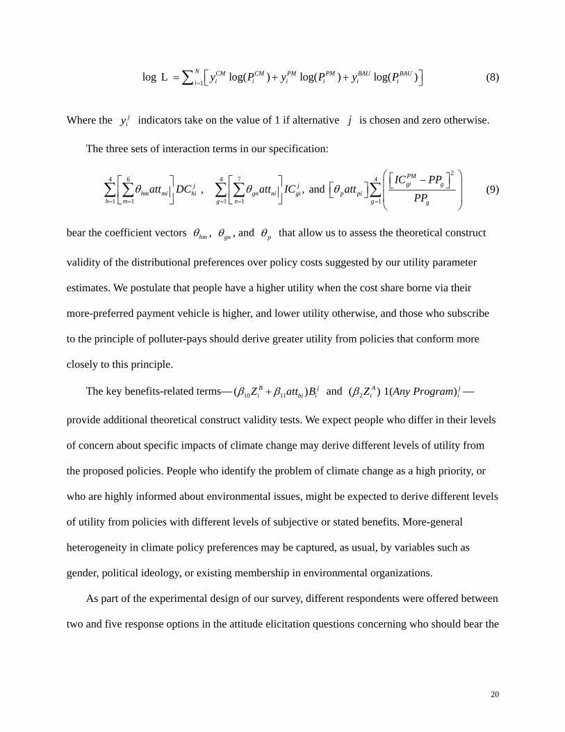
The log-likelihood function to be maximized with respect to the unknown parameters is then

20

1

log L log( ) log( ) log( )N CM CM PM PM BAU BAUi i i i i ii

y P y P y P= = + + ∑ (8)

Where the j

iy indicators take on the value of 1 if alternative j is chosen and zero otherwise. The three sets of interaction terms in our specification:

2

4 6 4 7 4

1 1 1 1 1 , , and

PMgi gj j

hm mi hi gn ni gi p pih m g n g g

IC PPatt DC att IC att

PPθ θ θ

= = = = =

− ∑ ∑ ∑ ∑ ∑ (9)

bear the coefficient vectors hmθ , gnθ , and pθ that allow us to assess the theoretical construct

validity of the distributional preferences over policy costs suggested by our utility parameter

estimates. We postulate that people have a higher utility when the cost share borne via their

more-preferred payment vehicle is higher, and lower utility otherwise, and those who subscribe

to the principle of polluter-pays should derive greater utility from policies that conform more

closely to this principle.

The key benefits-related terms— 10 11( )B ji bi iZ att Bβ β+ and 2( ) 1( )A j

i iZ Any Programβ —

provide additional theoretical construct validity tests. We expect people who differ in their levels

of concern about specific impacts of climate change may derive different levels of utility from

the proposed policies. People who identify the problem of climate change as a high priority, or

who are highly informed about environmental issues, might be expected to derive different levels

of utility from policies with different levels of subjective or stated benefits. More-general

heterogeneity in climate policy preferences may be captured, as usual, by variables such as

gender, political ideology, or existing membership in environmental organizations.

As part of the experimental design of our survey, different respondents were offered between

two and five response options in the attitude elicitation questions concerning who should bear the

21

costs of preventing climate change.28 A “neutral” option is not offered in all versions of the

survey instrument, so we cannot designate this as the omitted category in our specifications. The

neutral category, when it is available, can be aggregated with the “agrees” or “disagrees”

responses. It is sometimes the distinction between “agrees” and the omitted category of “does not

agree” that matters (that is, we define 1( ) 1hm hmatt Agree= = if the respondent explicitly agrees

and this indicator is zero otherwise). In other cases, the distinction between “disagrees” and

“does not disagree” does a better job of explaining the data (where we define

1( ) 1hm hmatt Disagree= = if the respondent explicitly disagrees and this alternative indicator is

zero otherwise).

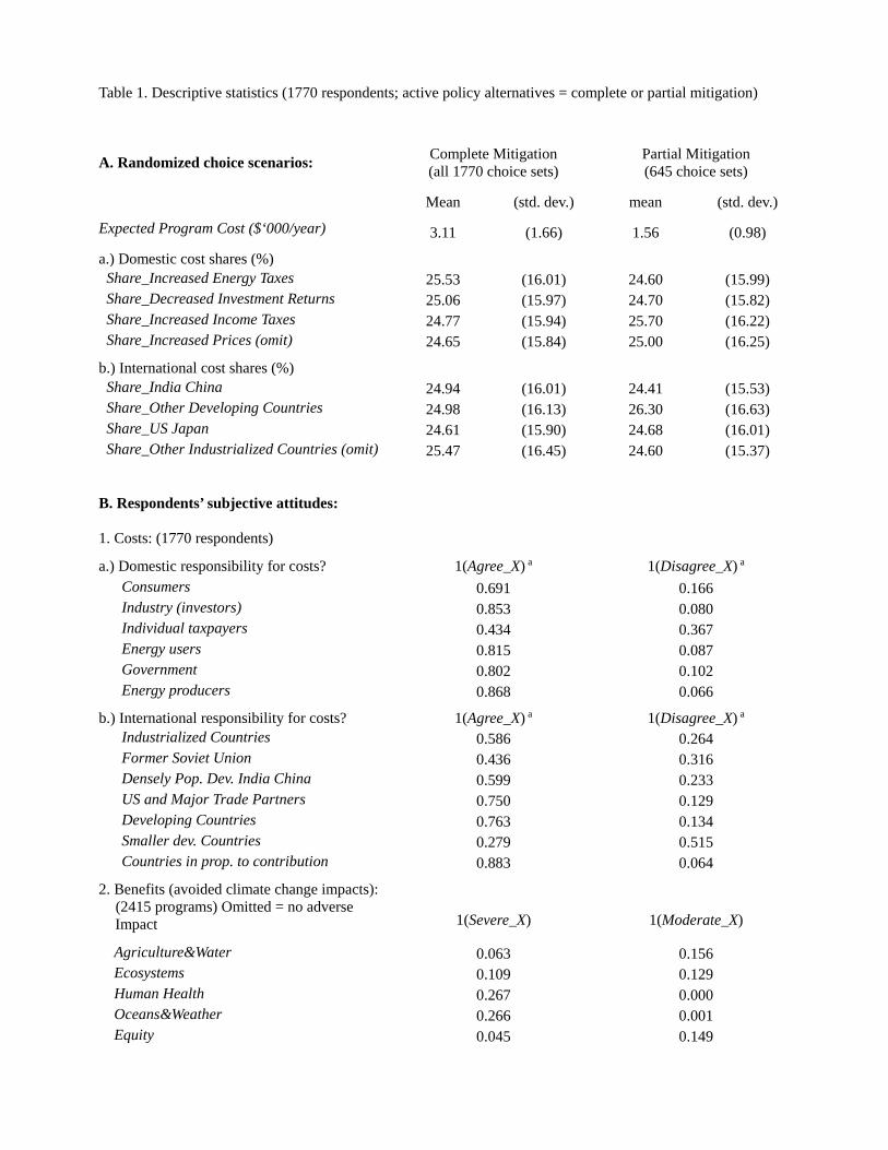
The descriptive statistics for the randomized choice scenario variables employed in our

models are reported in the top panel of Table 1, which summarizes the range of values used for

the costs of the climate change mitigation programs and the domestic and international

distributions of program costs.29 Multicollinearity among some of the attitudinal variables poses

a challenge for models which employ the whole set of attitudes about all potentially responsible

groups to shift the coefficients on each domestic cost share or international cost share. Rather

than including the universe of potential payers in each category (from the attitude questions

about responsibility) as shifters on every cost share in the corresponding category in the policy

28 Two-alternative versions offered only “agree” and “disagree”; three-alternative versions included “neutral”;

four-alternative versions dropped “neutral” but added “agree strongly” and “disagree strongly”; finally, the five-alternative versions reinstated the “neutral” option. To simplify our analysis, we combine the “strongly disagree” and ”disagree” categories (and likewise for “strongly agree” and “agree”).

29 This version of the paper includes descriptive statistics for more variables than are ultimately found to have statistically significant effects within our model. These summary statistics are provided for completeness. Where other variables in a class have been found to have estimated coefficient which are never remotely significantly different from zero, their coefficients have been set to zero in these models.

22

choice models, we simplify our model by matching each type of cost share to attitudes

concerning the responsibility of the most closely related group or groups.30

In the most general possible model, the potential benefits of each policy ( jB ) should

comprise all five available categories of anticipated impacts, including Agriculture & Water,

Oceans & Weather, Human Health, Ecosystems, and Equity. In our data, however, nearly seventy

percent of the respondents rated the Human Health impacts under BAU as “-4”, and about the

same percentage of this college sample rated the Oceans & Weather impacts as “-4” (see Online

Appendix Table B.1).

Our data on individual subjective climate change impacts are merely ratings on a symmetric

scale that runs from negative to positive. With subjective ratings, it is never clear which cardinal

scales different individuals may be using. Thus we convert the raw ratings from the survey into a

set of two coarse dummy variables for each type of impact: 1(Moderate) signifies a rating from

less than zero to “-2” (inclusive); 1(Severe) is a rating from less than “-2” to “-4” (inclusive). The

omitted category “no negative impact.” With this level of aggregation, virtually 99% of

respondents in this mostly student sample rated both the Human Health and Oceans & Weather

impacts as “severe.” As a result, we cannot estimate distinct marginal utilities associated with

these two categories of impacts for this sample. Instead, we use the alternative-specific indicator

variable 1( ) jiAny Program , shared by both the CM and PM alternatives to identify the common

“autonomous” component of utility from any of these programs, as well as the indicator

1( ) jiPartial Mitigation , activated only for the PM option (when it is offered).

30 Online Appendix Figure B.1 describes the way in which we elect to match the domestic variables for

theoretical construct validity assessment, and Figure B.2 explains the strategy for the international variables. The interaction terms between the cost share of a payment vehicle and the respondent’s attitudes toward the responsibility of that same type of payer thus constitute our working set of theoretical construct validity assessment variables (or, equivalently, our “distributional preference” variables).

23

The more-variable subjective impacts—for Agriculture & Water and for Ecosystems—are

also rather highly correlated. (See the degree of correlation in the detailed ratings for these two

types of impacts in Online Appendix Table B.2.)31 We opt to subsume the Agriculture & Water

impacts to a considerable extent under the Ecosystems impacts, and to use only Ecosystems

impacts and Equity impacts as our explicit benefits variables. The utility from any uncorrelated

components of the other three types of impacts will be absorbed by 1(Any Program) and

1(Partial Mitigation), which capture the autonomous utility from taking action against climate

change, regardless of the explicit costs or benefits used in our model.

IV. Estimation Results

Table 2 reports results for three different specifications. The first model assumes

homogeneous preferences, the second allows the estimated preference parameters to differ

systematically with a variety of the respondent’s attitudes about the responsibilities of different

parties to bear the costs of climate change mitigation, and with their stated concern about the

adverse distributional consequences of climate change if it is allowed to happen. Several other

types of heterogeneity are also entertained in this model. Finally, a third model pares down the

heterogeneous-preferences model to its essentials. After discussing our preferred parsimonious

specification, we devote a brief subsection to commentary on the consequences of other

modeling strategies we have explored with these data.

31 To accommodate these collinearities, we have explored models which rotate through a set of three basic

models. In each specification, we “feature” just one of these three types of impacts. In each model, we acknowledge that the estimated marginal utilities on the featured impact will subsume the covarying portions of other correlated impacts, while the common effects will be absorbed by the alternative-specific dummy variables. While it would have been appealing to be able to identify clearly the distinct effects of each type of impact, it is not really possible to do so with these data. However, weight-of-the-evidence inferences can still be deduced from these more-aggregated versions of the different subjective impacts.

24

A. Conditional Logit Models

Model 1 uses as explanatory variables only the cost of the program, the stated domestic and

international cost share variables, the individual’s subjective benefits (avoided impacts), the

indicator 1(Any Program) and the indicator 1(Partial Mitigation), with the coefficient for this

last variable relegated to the Appendix table of incidental parameters. This model therefore

assumes that preferences are homogeneous and that choices across policy alternatives are driven

only by the size and distribution of policy costs and the individual’s perceptions of the

consequences of climate change should a policy of BAU be followed. Our concern in this paper

is that the assumption of homogeneous preferences may be untenable, and may mask the

presence of important types of heterogeneity.

As noted, our study differs from most other SP assessments of policy preferences in that our

choice scenarios include a randomized specific mix of payment vehicles in the form of domestic

cost shares and a randomized specific mix of international cost shares for the proposed policies.

In estimation, of course, one of the cost shares in each category must be omitted to avoid perfect

multicollinearity with the alternative-specific dummy variables for “Any Program” and the PM

alternative (when it is offered). With homogeneous preferences, among all the cost variables in

Model 1, only the magnitude of program costs is statistically significant. There is no apparent

effect from the domestic or international distributions of program costs.

In contrast, the benefits variables—the indicators for avoided severe impacts on Ecosystems

and Equity, and for avoided moderate impacts on Equity, along with the generic implicit benefits

associated with 1(Any Program) (as opposed to BAU)—are all individually statistically

significant and bear the anticipated signs and relative magnitudes. However, we suspect in Model

1 that failure to allow for heterogeneous preferences with respect to domestic and international

25

cost shares may preclude our ability to detect how WTP for climate change mitigation varies

with these distributional consequences.

Model 2 introduces heterogeneity in distributional preferences according to the

best-matching attitudes our survey elicits concerning the degree of responsibility of different

domestic and international groups to bear the costs of climate change mitigation. We use the

symbol “►” to highlight all the interaction terms based on distributional attitudes in this table.32

We also introduce an indicator for each respondent’s separately elicited degree of worry about

the potential regressivity of climate change impacts, should they be allowed to proceed under a

policy of BAU.33

Section (i) of Model 2 reveals that when we allow for preference heterogeneity by

permitting the estimated marginal utilities to vary with respondents’ attitudes about which groups

should be held responsible for the costs of climate change mitigation, domestic cost shares borne

through energy taxes and investment returns are revealed to be very important to some segments

of the population. Those who agree that energy users should bear the costs of climate change

mitigation derive greater utility (and are thus more willing to pay) for programs where a larger

share of domestic costs is borne through energy taxes. Those who disagree that taxpayers should

foot the bill derive less utility (and are hence less willing to pay) for programs which make

relatively greater use of energy taxes as their payment vehicle. For the average of all other

attitudinal categories (i.e. the baseline), it appears that variations in the share of costs borne

through increased energy taxes does not have a statistically significant effect on utility.

32 Online Appendix Table B.3 shows that these attitudes are most closely related to political ideology, rather

than income or employment status. 33 To conserve space, we do not report the results of our numerous preliminary specifications which led us to

this working model. We retain only those variables and interaction terms which are significant in some or all of our exploratory models.

26

For the international cost share variables in Section (i) of Model 2, for most types of

respondents, there is little evidence of sensitivity to (a) different international cost shares or

(b) departures from the set of international shares that would correspond to the “polluter-pays”

distribution of costs. However, respondents who explicitly disagree that the costs of climate

change mitigation should be borne by “densely populated developing countries such as India and

China” seem to experience lower utility when a larger share of international costs accrue to these

two countries. Although the t-test statistic on this parameter estimate is just less than 1.6, this

coefficient is fairly stable and occasionally significant at the 10% level in alternative

specifications, so we retain it as we simplify our model.

For respondents who agree that the costs of climate change should be borne internationally

by the U.S. and Japan, programs where a larger share of the cost is borne by these countries may

confer greater utility. Again, although the t-test statistic for this estimate is only about 1.4, the

coefficient comes close to being statistically significant at the 10% level in some other

specifications, so we retain it in our models as well.

Concerning the final variables in Section (i) of Model 2—involving the index intended to

capture departures from the polluter-pays shares of international costs—none of these variables

is individually significant. The baseline effect is not different from zero and the effect appears

not to be shifted in any systematic direction by attitudes about whether countries should be held

responsible “in proportion to their contribution to the problem.” The polluter-pays index is

constructed using the same shares that also appear individually in the model, so one might expect

some duplication when both types of variables are included in the same model. However, the

27

polluter-pays index is not individually significant even when the individual international cost

shares are dropped, so we omit these terms from further analyses.34

Model 3 in Table 2 is our preferred specification. Compared to Model 2, we drop some

statistically very insignificant variables with near-zero estimated point values to enhance the

precision with which we can calculate the sampling distribution of willingness-to-pay implied by

the jointly normally distributed maximum likelihood parameter estimates. Aside from these

modifications, the key results from Model 2 are relatively robust. The key attitudinal shifter on

the international cost share borne by the US and Japan becomes statistically significant at the 10%

level, and the maximized value of the log-likelihood function changes only trivially between

Models 2 and 3.35

There seems to be a clear lesson from these empirical results (with respect to the cost of the

policy, and the domestic and international incidence of these costs). For some classes of

consumers, the utility derived from a climate change mitigation policy (and thus willingness to

pay for it) depends strongly upon the distributional consequences of the policy in terms of who

will bear its costs. There is considerable heterogeneity across the population in the degree of

sensitivity to the incidence of a policy’s costs. This sensitivity is unambiguous in the case of

domestic costs. For international shares, the results are less striking, but still suggestive. The

general lack of sensitivity to international cost shares (compared to domestic cost shares) is

notable—except for the cost share for the U.S. and Japan (which increases support for the policy

34 It may simply be that respondents are not generally aware of the actual proportional contributions of these

country groups to the production of greenhouse gases. Alternatively, what they perceive is based not only on the emissions record of the year 2000, but also historically.

35 Despite their individual statistical insignificance, we retain the baseline effects for the domestic cost shares. Their point values are non-trivially different from zero even if the standard errors of these estimates are rather large. While these parameters cannot be estimated precisely, forcing their point values to zero by dropping the baseline effects from the model tends to produce implausible values for WTP in some of our simulations. We do, however, drop the baseline effects for two of the international cost shares (for “Other Developing Countries” and “US and Japan”) because compared to the coefficients on other share variables, their point estimates are tiny as well as their t-test statistics.

28

when the individual agrees that these countries have a responsibility to bear the costs of climate

change mitigation policies).

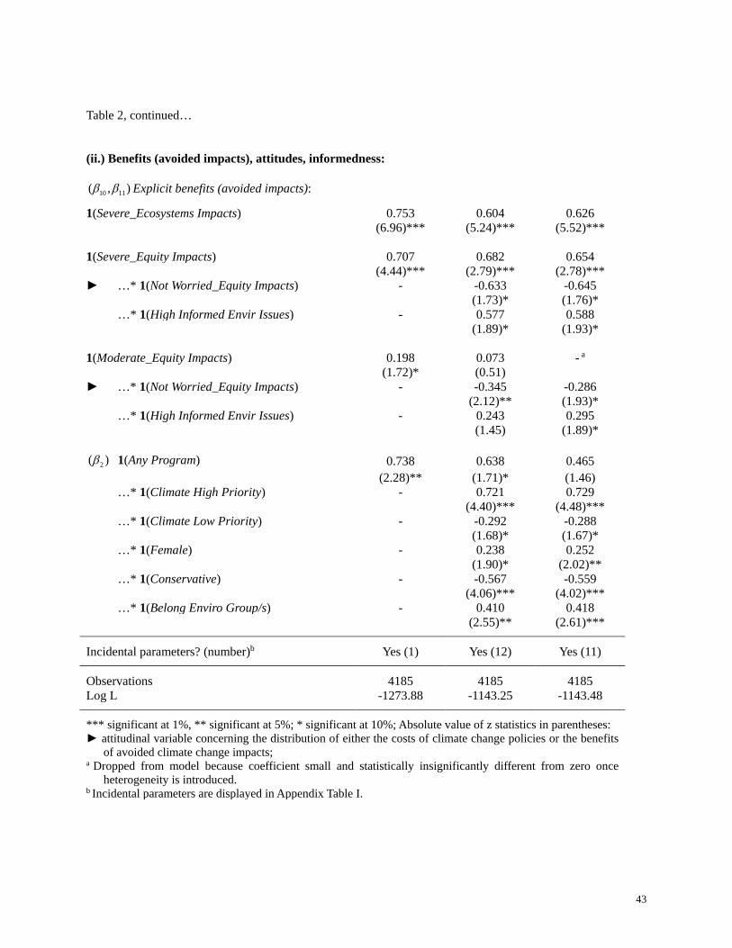
Besides the effects of distributional preferences concerning the costs of a given climate

policy, a number of other attitude-based interaction terms also deserve our attention. In part (ii.)

of Table 2, we note first that respondents who anticipate severe ecosystems impacts from climate

change under BAU derive statistically significantly greater utility from climate change

mitigation, as expected (although this utility also captures correlated impacts on Agriculture and

Water, and other anticipated climate change impacts are subsumed under our alternative-specific

constants). However, for respondents who state explicitly that they are not worried about the

regressivity of climate change impacts, the increment to utility from a policy that avoids severe

equity impacts is negative. Its size is also sufficient to offset the positive average utility from

avoiding these equity impacts for respondents who do care about them or are neutral about the

issue. Being unworried about moderate equity impacts also significantly decreases the utility to

be derived from such a policy.

The respondent’s subjective level of informedness about environmental issues also has

detectible effects on the utility consequences of avoiding severe or moderate equity impacts from

climate change. This informedness effect is roughly twice as large for severe equity impacts

(regressivity) as for moderate equity impacts.

Finally, the autonomous utility associated with 1(Any Program)—independent of the

model’s explicit costs and explicit ecosystem or equity benefits of the policy—varies

systematically with a number of additional respondent attitudes and characteristics. Not

surprisingly, any type of climate change mitigation program confers more utility if the individual

considers climate change to be a high-priority problem and less if it is considered to be a

low-priority problem among other global concerns. Women derive more utility from any kind of

29

climate change mitigation policy and self-identification as a conservative is associated with less

utility from climate change mitigation. Membership in one or more environmental groups is also

associated with greater autonomous utility from any type of climate change mitigation. To the

extent that these findings conform to casual empiricism, we can treat them as support for the

theoretical construct validity of the stated preferences elicited by our survey.36

B. Other Specifications

We have also estimated the preference parameters for our sample of respondents using latent

class models with two and three classes of preferences, as well as a selection of mixed logit

(fixed and random parameters) models, and hierarchical Bayes models. We have also estimated a

mixed logit model that accomplishes the same modeling objective as a nested logit

specification—namely, one with a zero-mean random coefficient on the 1(Any Program)

indicator variable. None of these alternative specifications dominates the conditional logit

models featured in this paper. Consequently, we relegate these results to Online Appendix B.

V. Implied Willingness to Pay for Climate Change Mitigation

The systematic variations in marginal utility parameters that we identify in Table 2 translate

into corresponding systematic variation in the implied maximum willingness to pay for climate

change mitigation policies with different attributes. For this paper, the key policy attributes

include policy costs and differences in the incidence of these costs both domestically and

internationally. Willingness to pay will also differ across individuals with different subjective

assessments of the likely severity of climate change under a policy of BAU and different

attitudes about those possible climate change impacts, different degrees of familiarity with

36 The appendix reports and discusses the additional incidental parameters associated with Models 1, 2, and 3.

30

environmental issues (or membership in environmental groups), and different prioritizations of

climate change among other global problems.

Many different dimensions of variability are captured in our estimating models in Table 2.

To illustrate some of the implied effects on WTP for climate change policies from this

heterogeneity, we will explore some selected simulations of the fitted WTP distribution under

different conditions—(a.) different domestic and international distributions of policy costs,

(b.) different subjective climate change impacts and equity consequences, (c.) different attitudes

about responsibility and regressivity, and (d.) different types of individuals. For these simulations,

we will use Model 3 in Table 2. Note that these are not fitted WTP estimates for the entire

sample, or for any subsample, of the data. Instead, they are predicted WTP distributions for

prototypical individuals with specified characteristics and attitudes, facing specified types of

climate policies. The distribution reflects estimation precision (i.e. the variance-covariance

matrix) for the estimated maximum likelihood parameters in Model 3.37

To calculate a point value for willingness to pay under a specified set of conditions (i.e. a

set of values for the model’s explanatory variables), we set to zero the indirect utility difference

in equation (6) and solve for the policy cost that would produce this indifference. Table 3 presents

simulated distributions of WTP, for point values calculated for each of 1000 random draws from

the asymptotically joint normal distribution of the estimated maximum likelihood parameters of

Model 3. To put these amounts in perspective, the median annual income, across the 1770

individuals who reported their household income (typically the income in their parental

household), is about $62,000. The corresponding monthly income, against which these WTP

estimates should be compared, is thus about $5200.

37 Note that we cannot merely report what fraction of the sample was willing to pay a given cost for climate

change mitigation because costs, the cost distribution, and the subject’s perceptions of climate change impacts and equity consequences differ across questionnaires.

31

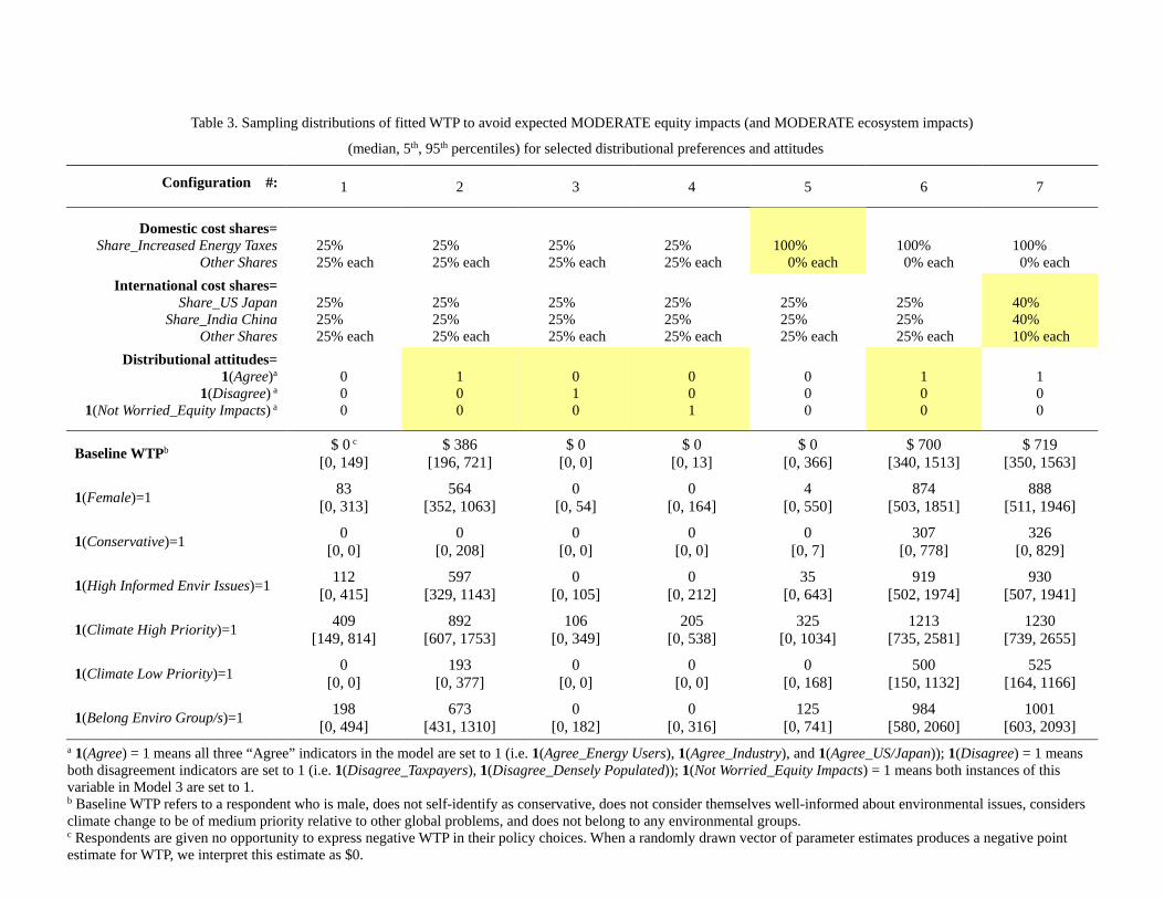
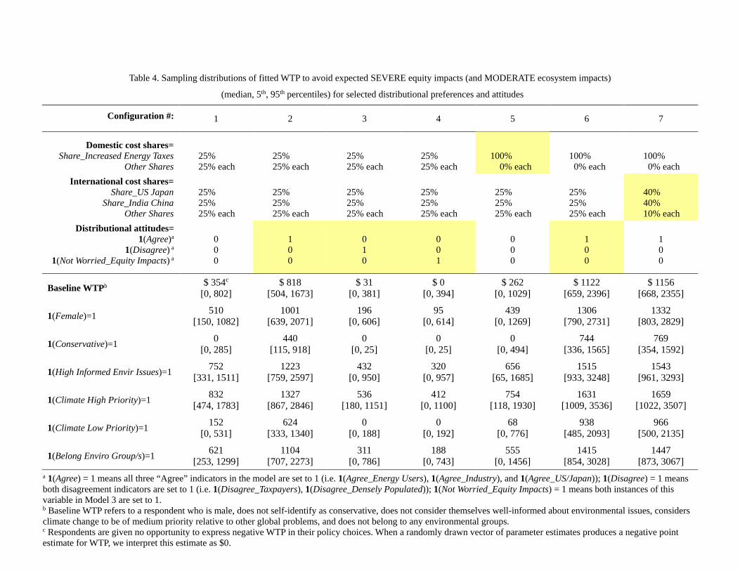
Simulations when equity impacts are expected to be moderate

In Table 3, we simulate distributions of WTP for a policy of complete mitigation for a

respondent who expects no more than moderate Ecosystem impacts and moderate Equity

impacts, and who sees only two alternatives: CM versus BAU.38 We build these distributions for

seven different configurations of cost shares and distributional attitudes. For each configuration,

we begin with the simulated distribution of “Baseline WTP.” This distribution applies for a

respondent who is male, does not self-identify as conservative, does not consider himself

well-informed about environmental issues, considers climate change to be of medium priority

relative to other global problems, and does not belong to any environmental groups. In the rows

of the table below the Baseline WTP for each configuration, we show how the predicted

distribution of WTP changes as these characteristics of the respondent are changed, one at a

time.39

WTP is not constrained to be non-negative in our models, but there is also no opportunity in

the survey for any respondent to express negative WTP, so any simulated point values of WTP

which are negative are converted to zero.40 The first entry under Configuration 1 in Table 3

reveals that if all shares are equal, and if respondents do not explicitly agree or disagree with any

of the statements about responsibility to bear the costs of mitigation, then there is little evidence

of any positive willingness to pay for climate change mitigation programs. The 90% interval for

WTP excludes zero only for the case where climate change is acknowledged to be a high priority

policy issue, although median WTP is positive if our stylized respondent is female,

38 Of course, our model is capable of simulating WTP for the prevention of impacts of different levels of severity, or for partial, rather than complete mitigation. To illustrate its capabilities, however, we focus on the CM policy, since all respondents were asked about this scenario versus BAU, while only a subset also saw the partial mitigation alternative.

39 Of course, two or more of these indicators could be changed simultaneously. Since space constraints limit the number of simulations we can use as illustrations, however, we limit these illustrations to single changes.

40 This is analogous to the econometric conventions adopted for Tobit-type models, where the latent dependent variable can be negative, but the probability in the negative domain is converted to a point mass at zero before the conditional expectation of the dependent variable is calculated.

32

well-informed about environmental issues, sees climate change as a high-priority policy issue, or

belongs to at least one environmental group.

In Configuration 2, we switch on just the “ Agree” indicators (i.e. 1(Agree_ Energy Users)

= 1, 1(Agree_ Industry) = 1, and 1(Agree_ US/Japan) = 1). These distributional preferences

result in a strictly positive 90% interval for WTP for the Baseline case and all others, unless the

baseline individual is conservative or believes that climate change is a low-priority policy

concern. In contrast, consider Configuration 3, where we switch off the “ Agree” indicators (i.e.

set 1(Agree_ Energy Users) = 0, 1(Agree_ Industry) = 0, and 1(Agree_ US/Japan) = 0) and

switch on the “ Disagree” indicators (i.e. 1(Disagree_ Taxpayers) = 1 and 1(Disagree_ Densely

Populated) = 1). Alternatively, in Configuration 4, we leave both the “ Agree” and “ Disagree”

indicators set to zero and use 1(Not Worried_Equity/Fairness)=1. In Configurations 3 and 4, the

90% interval for WTP again includes zero in all cases and the median is non-zero only if climate

change is considered a high-priority issue.

Configuration 5 restores the same conditions as in Configuration 1, except it uses a domestic

payment vehicle that is 100% energy taxes. This would be the case if a carbon tax were to be

used as the payment vehicle for climate policy. Zero is now within the 90% interval for WTP for

all cases, and the median values, where they are non-zero, are now smaller. There is, however,

greater dispersion in the simulated WTP distribution.

Configuration 6 replicates Configuration 2, but again shifts all of the domestic costs to

energy taxes. Alternatively, one can compare Configuration 6 to Configuration 5, where the

difference stems from activating all of the “ Agree” indicators. Either way of looking at this

change makes a dramatic difference in WTP. For Configuration 6, all of the 90% intervals are

33

substantially greater than zero, with the exception of the conservative case, where the median is

$307 per month but the 5th percentile is zero.

Finally, Configuration 7 retains the other conditions for Configuration 6, but illustrates the

consequences of increasing the international cost shares for India and China, and for the US and

Japan, from 25% to 40% each. This adjustment increases median WTP, but only by amounts on

the order of $10 to $25.

Table 3 thus demonstrates that if climate change impacts on equity are expected to be only

moderate, then WTP to prevent climate change will be essentially zero for many types of

consumers. However, certain types of consumers will be willing to pay substantial amounts if

they specifically agree with the payment vehicle to be employed and the responsibility of the

international country groups which will bear the costs of mitigation.41

Simulations when equity impacts are expected to be severe

In contrast to the modest WTP amounts for most types of consumers when expected climate

change impacts on Equity are only moderate, we can now consider what happens for those

individuals who believe that climate change will have severe impacts on Equity. We retain the

assumption of no more than moderate (i.e. non-severe) impacts upon Ecosystems. These

simulations are presented in Table 4, where the 49 illustrative simulations are analogous to those

presented in Table 3. As expected, if Equity impacts are judged to be severe, rather than just

moderate, WTP will tend to be higher—sometimes much higher. For Configuration 1, for

example, Baseline WTP now has a median value of $354 per month, rather than $0. Comparing

41 It is tempting to consider calculating a marginal rate of substitution (MRS) between the different domestic cost shares (i.e. a ratio of marginal utilities), as has been suggested to us by Roberton Williams. One would need to simulate this MRS in the same manner as we calculate WTP (the special case of the marginal rate of substitution between a specified program and income). Such an MRS would have to be derived with caution, however, since our model demonstrates that it will vary markedly with the attitudinal shifters (and may be indeterminate in cases where the distribution of the parameter in the dominator does not exclude zero). Fortunately, the marginal utility of income parameter used in the denominator of our WTP calculations, 1α , seems to be located well away from zero.

34

Table 4 to Table 3 reveals that distributional preferences have an even greater impact on WTP

for different types of climate change policies.42

VI. Caveats and Conclusions

We use a sample made up primarily of students drawn from over ninety different colleges

and universities across the United States and Canada. Our sample is not representative of the

entire population, so it is not suitable for predicting society’s overall average or aggregate

willingness to pay for climate change mitigation. Instead, we use this relatively young sample to

demonstrate empirically that the distributional consequences of alternative climate change

policies can strongly influence policy preferences.43 The domestic distribution of mitigation

costs, and the regressivity of perceived climate change impacts in the absence of mitigation, both

have strongly significant effects on individual willingness to pay. There is evidence to suggest

that the international distribution of mitigation costs may also matter, although the “polluter pays”

principle does not seem to be supported by the preferences of our subjects.

The impact of these distributional consequences depends on whether they conform to, or

conflict with, each individual’s normative opinions about (a.) which groups should bear the

responsibility for mitigation costs and (b.) whether the burden of climate change impacts borne

by the world’s poor, in the absence of mitigation, is a cause for concern.

42 A word on the estimated magnitudes of WTP for climate change mitigation is appropriate at this point.

Recall that these WTP estimates pertain to a policy of CM. To maintain the global climate at current levels, it may indeed be the case that huge costs would need to be incurred. It is more likely that a policy of PM would be adopted, if any action at all is undertaken. The simulated WTP values in Tables 3 and 4 must be considered relative to a household income on the order of $5000 per month. The WTP estimates derived from this sample are of similar magnitude to those in Lee and Cameron (2008). Also, for their web-based survey of a sample of roughly 250 Harvard graduate students in law and public policy, Viscusi and Zeckhauser (2006) find that median WTP to prevent climate change is about 3% of income (and the mean was 6%). They estimate that average expected income for these students is something like $150,000 per year, which implies that median WTP would be about $4500 and mean WTP would be about $9000.

43 For estimates of WTP for climate change mitigation, based on an analogous general population mail survey sample with careful sample selection corrections, see the quantitative results in Lee and Cameron (2008)

35

Our findings also highlight the tenuousness of the common assumption that it is possible to

conduct an assessment of the likely efficiency of a proposed policy (i.e. a benefit-cost analysis)

that is entirely separate from any subsequent consideration of the equity consequences of that

policy. Distributional consequences can have a huge impact on WTP for some types of people. In

fact, it may not be possible to adequately specify a policy independent of its distributional

consequences. If a stated preference survey fails to mention the anticipated distributional

consequences of a proposed policy, respondents are at liberty to impute whatever unspecified

distributional consequences seem most probable to them, and such perceptions may differ across

people in unobserved ways. A complete choice scenario should probably include an explicit

statement about the expected distributional consequences of the policy, perhaps randomized so

that it is possible to model how these consequences systematically affect WTP. It remains an

open question whether there is any range of circumstances under which we can produce a single

WTP value for a policy, without fully stipulating the distributions of benefits and costs.

In addition to our main findings about the dependence of willingness to pay on normative

notions of who should pay the costs or enjoy the benefits of climate change mitigation policies,

we highlight some additional sources of significant heterogeneity in climate policy preferences.

Individuals who consider themselves to be relatively better-informed about environmental issues

are willing to pay markedly more to prevent the adverse effects of climate change upon the

world’s poor. Those who already belong to at least one environmental group, those who believe

that the climate problem is an important policy priority, and women, are all willing to pay more

to prevent climate change, whereas self-identifying conservatives and those who believe climate

change is a low priority are willing to pay much less.

Our findings also highlight the important role of climate change advocacy. Our results

confirm a strong correlation between attitudes and willingness to pay. Economists are generally

36

more confident that people’s choices can be reliably altered when some policy measure modifies

the constraints that they face, but climate advocates work to alter choices by changing people’s

preferences. This can be accomplished by changing people’s subjective perceptions about the

consequences of climate change, or by changing their attitudes towards these consequences.

Overall, our research confirms that the public’s perceptions about the likely incidence of

costs and benefits of any specific climate change mitigation policy will affect support for that

policy. There is unlikely to be any single policy that will be supported by everyone, since people

have markedly different normative opinions about what distribution of cost or benefits is

desirable. In some cases, these normative opinions may be self-serving, and in others they may

be altruistic. Trying to estimate a single overall average willingness to pay to prevent climate

change may be ill-advised, since willingness to pay is clearly zero for some types of people, but

may be very high for others. Finally, we emphasize that any type of climate change policy—from

business-as-usual through complete mitigation—has the potential to create vastly different

distributions of welfare, both across society and across regions. Distributional changes can lead

to conflict, especially when various groups have different opinions about who should bear the

responsibility for policy costs or enjoy the policy’s benefits. A fuller understanding of the

implications of specific climate change policies for potential future conflict is vital to making

prudent public policy choices among the available options.

References:

Anthoff, D, Hepburn, C and Tol, RSJ (2009) Equity weighting and the marginal damage costs of climate change. Ecolog. Econ. 68(3):836-849.

Arrow, K, Solow, R, Portney, PR, Leamer, EE, Radner, R and Schuman, H (1993) Report of the NOAA Panel on Contingent Valuation. Federal Register 58(10):4601-4614.

Azar, C and Sterner, T (1996) Discounting and distributional considerations in the context of global warming. Ecolog. Econ. 19(2):169-184.

Bergstrom, JC, Boyle, KJ and Yabe, M (2004) Trading taxes vs. paying taxes to value and finance public environmental goods. Environ. Resource Econ. 28(4):533-549.

Berrens, RP, Bohara, AK, Jenkins-Smith, H, Silva, C and Weimer, DL (2003) The advent of Internet surveys for political research: A comparison of telephone and Internet samples. Political Analysis 11(1):1-22.

Berrens, RP, Bohara, AK, Jenkins-Smith, H, Silva, CL, Ganderton, P and Brookshire, D (1998) A joint investigation of public support and public values: the case of instream flows in New Mexico. Ecolog. Econ. 27(2):189-203.

Berrens, RP, Bohara, AK, Jenkins-Smith, HC, Silva, CL and Weimer, DL (2004) Information and effort in contingent valuation surveys: application to global climate change using national internet samples. J. Environ. Econ. Manage. 47(2):331-363.

Bosello, F, Roson, R and Tol, RSJ (2006) Economy-wide estimates of the implications of climate change: Human health. Ecolog. Econ. 58(3):579-591.

Burghart, DR, Cameron, TA and Gerdes, GR (2007) Valuing publicly sponsored research projects: Risks, scenario adjustments, and inattention. J. Risk Uncertainty 35(1):77-105.

Cameron, TA (2005) Individual option prices for climate change mitigation. J. Public Econ. 89(2-3):283-301. Cameron, TA (2005) Updating subjective risks in the presence of conflicting information: An application to climate

change. J. Risk Uncertainty 30(1):63-97. Cameron, TA and Gerdes, GR (2005) Individual subjective discounting: form, context, format, and noise.

Unpublished manuscript, Department of Economics, University of Oregon:52 pp. Cameron, TA and Gerdes, GR (2006) Discounting versus risk aversion: their effects on individual demands for

climate change mitigation. Unpublished manuscript, Department of Economics, University of Oregon:56 pp.

Champ, PA, Flores, NE, Brown, TC and Chivers, J (2002) Contingent valuation and incentives. Land Econ. 78(4):591-604.

de Blaeij, A, Florax, R, Rietveld, P and Verhoef, E (2003) The value of statistical life in road safety: a meta-analysis. Accident Analysis and Prev. 35(6):973-986.

DeShazo, JR and Fermo, G (2002) Designing choice sets for stated preference methods: The effects of complexity on choice consistency. J. Environ. Econ. Manage. 44(1):123-143.

Diamond, PA and Hausman, JA (1994) Contingent valuation - Is some number better than no number? J. Econ. Perspect. 8(4):45-64.

Dietz, S and Stern, N (2008) Symposium: The Economics of Climate Change: The Stern Review and Its Critics: Why Economic Analysis Supports Strong Action on Climate Change: A Response to the Stern Review's Critics. Rev. Environ. Econ. Pol. 2(1):94-113.

38

Florax, R, Travisi, CM and Nijkamp, P (2005) A meta-analysis of the willingness to pay for reductions in pesticide risk exposure. Europ. Rev. Agr. Econ. 32(4):441-467.

Flores, NE (2002) Non-paternalistic altruism and welfare economics. J. Public Econ. 83(2):293-305. Flores, NE and Strong, A (2007) Cost credibility and the stated preference analysis of public goods. Resource

Energy Econ. 29(3):195-205. Hanley, N, Grande, J, Álvarez-Farizo, B, Salt, C and Wilson, M (2001) Risk perceptions, risk-reducing behaviour

and willingness to pay: radioactive contamination in food following a nuclear accident. Working Paper, Department of Economics, University of Glasgow.

Hensher, DA (2006) Revealing differences in willingness to pay due to the dimensionality of stated choice designs: An initial assessment. Environ. Resource Econ. 34(1):7-44.

Johnson, LT (2006) Distributional preferences in contingent valuation surveys. Ecolog. Econ. 56(4):475-487. Jorgensen, BS and Syme, GJ (2000) Protest responses and willingness to pay: attitude toward paying for stormwater

pollution abatement. Ecolog. Econ. 33(2):251-265. Kelly, DL, Kolstad, CD and Mitchell, GT (2005) Adjustment costs from environmental change. J. Environ. Econ.

Manage. 50(3):468-495. Kinnell, J, Lazo, JK, Epp, DJ, Fisher, A and Shortle, JS (2002) Perceptions and values for preventing ecosystem

change: Pennsylvania duck hunters and the Prairie Pothole Region. Land Econ. 78(2):228-244. Krutilla, K (2005) Using the Kaldor-Hicks tableau format for cost-benefit analysis and policy evaluation. J. Policy

Anal. Manage. 24(4):864-875. Kurukulasuriya, P, Mendelsohn, R, Hassan, R, Benhin, J, Deressa, T, Diop, M, Eid, HM, Fosu, KY, Gbetibouo, G,

Jain, S, Mahamadou, A, Mano, R, Kabubo-Mariara, J, El-Marsafawy, S, Molua, E, Ouda, S, Ouedraogo, M, Sene, I, Maddison, D, Seo, SN and Dinar, A (2006) Will African agriculture survive climate change? World Bank Econ. Rev. 20(3):367-388.

Lange, A (2006) The impact of equity-preferences on the stability of international environmental agreements. Environ. Resource Econ. 34(2):247-267.

Lange, A, Vogt, C and Ziegler, A (2007) On the importance of equity in international climate policy: An empirical analysis. Energy Econ. 29(3):545-562.

Laughland, AS, Musser, WN, Shortle, JS and Musser, LM (1996) Construct validity of averting cost measures of environmental benefits. Land Econ. 72(1):100-112.

Lee, JJ and Cameron, TA (2008) Popular support for climate change mitigation: Evidence from a general population mail survey. Environ. Resource Econ. 41(2):223-248.

Li, H, Berrens, RP, Bohara, AK, Jenkins-Smith, HC, Silva, CL and Weimer, DL (2004) Would developing country commitments affect us households' support for a modified Kyoto Protocol? Ecolog. Econ. 48:329-343.

Mendelsohn, R (2008) Symposium: The Economics of Climate Change: The Stern Review and Its Critics: Is the Stern Review an Economic Analysis? Rev. Environ. Econ. Pol. 2(1):45-60.

Mendelsohn, R, Dinar, A and Williams, L (2006) The distributional impact of climate change on rich and poor countries. Environ. Devel. Econ. 11:159-178.

Morrison, MD, Blamey, RK and Bennett, JW (2000) Minimising payment vehicle bias in contingent valuation studies. Environ. Resource Econ. 16(4):407-422.

Nordhaus, WD (2007) A Review of the Stern Review on the Economics of Climate Change. J. Econ. Lit. 45(3):686-702.

39

Parks, BC and Roberts, JT (2006) Globalization, vulnerability to climate change, and perceived injustice. Society Natural. Res. 19(4):337-355.

Raymond, L (2006) Cutting the "Gordian knot" in climate change policy. Energy Pol. 34(6):655-658. Reibstein, R (2005) Ethics, equity and international negotiations on climate change. Ecolog. Econ. 52(4):545-546. Rollins, K (1997) Wilderness canoeing in Ontario: Using cumulative results to update dichotomous choice

contingent valuation offer amounts. Can. J. Agr. Econ. 45(1):1-16. Schade, C, Kunreuther, H and Kaas, KP (2002) Low-probability insurance decisions: The role of concern. Wharton

Risk Center Working Paper Nr. 02-10-HK, Wharton School, University of Pennsylvania. Schlapfer, F (2006) Survey protocol and income effects in the contingent valuation of public goods: A meta-analysis.

Ecolog. Econ. 57(3):415-429. Stephan, G and Muller-Furstenberger, G (2004) Does distribution matter? Efficiency, equity and flexibility in

greenhouse gas abatement. Environ. Resource Econ. 27(1):87-107. Stern, N (2006). The economics of climate change: The Stern Review. Cambridge University Press, New York. Sterner, T and Persson, UM (2008) Symposium: The Economics of Climate Change: The Stern Review and Its

Critics: An Even Sterner Review: Introducing Relative Prices into the Discounting Debate. Rev. Environ. Econ. Pol. 2(1):61-76.

Stevens, TH, DeCoteau, NE and Willis, CE (1997) Sensitivity of contingent valuation to alternative payment schedules. Land Econ. 73(1):140-148.

Thomas, DSG and Twyman, C (2005) Equity and justice in climate change adaptation amongst natural-resource-dependent societies. Global Environ. Change-Human Pol. Dimen. 15(2):115-124.

Viscusi, WK and Zeckhauser, RJ (2006) The perception and valuation of the risks of climate change: A rational and behavioral blend. Climatic Change 77:151-177.

Weitzman, ML (2007) A Review of the Stern Review on the Economics of Climate Change. J. Econ. Lit. 45(3):703-724.

Weyant, JP (2008) Symposium: The Economics of Climate Change: The Stern Review and Its Critics: A Critique of the Stern Review's Mitigation Cost Analyses and Integrated Assessment. Rev. Environ. Econ. Pol. 2(1):77-93.

Whitehead, JC, Blomquist, GC, Ready, RC and Huang, JC (1998) Construct validity of dichotomous and polychotomous choice contingent valuation questions. Environ. Resource Econ. 11(1):107-116.

Table 1. Descriptive statistics (1770 respondents; active policy alternatives = complete or partial mitigation)

A. Randomized choice scenarios:

Complete Mitigation (all 1770 choice sets)

Partial Mitigation (645 choice sets)

Mean (std. dev.) mean (std. dev.)

Expected Program Cost ($‘000/year) 3.11 (1.66) 1.56 (0.98)

a.) Domestic cost shares (%) Share_Increased Energy Taxes 25.53 (16.01) 24.60 (15.99) Share_Decreased Investment Returns 25.06 (15.97) 24.70 (15.82) Share_Increased Income Taxes 24.77 (15.94) 25.70 (16.22) Share_Increased Prices (omit) 24.65 (15.84) 25.00 (16.25)

b.) International cost shares (%) Share_India China 24.94 (16.01) 24.41 (15.53) Share_Other Developing Countries 24.98 (16.13) 26.30 (16.63) Share_US Japan 24.61 (15.90) 24.68 (16.01) Share_Other Industrialized Countries (omit) 25.47 (16.45) 24.60 (15.37)

B. Respondents’ subjective attitudes:

1. Costs: (1770 respondents)

a.) Domestic responsibility for costs? 1(Agree_X) a 1(Disagree_X) a Consumers 0.691 0.166 Industry (investors) 0.853 0.080 Individual taxpayers 0.434 0.367 Energy users 0.815 0.087 Government 0.802 0.102 Energy producers 0.868 0.066

b.) International responsibility for costs? 1(Agree_X) a 1(Disagree_X) a Industrialized Countries 0.586 0.264 Former Soviet Union 0.436 0.316 Densely Pop. Dev. India China 0.599 0.233 US and Major Trade Partners 0.750 0.129 Developing Countries 0.763 0.134 Smaller dev. Countries 0.279 0.515 Countries in prop. to contribution 0.883 0.064

2. Benefits (avoided climate change impacts): (2415 programs) Omitted = no adverse Impact

1(Severe_X)

1(Moderate_X)

Agriculture&Water 0.063 0.156 Ecosystems 0.109 0.129 Human Health 0.267 0.000 Oceans&Weather 0.266 0.001 Equity 0.045 0.149

41

Table 1, continued

3. Respondent individual characteristics: (1770 respondents)

a.) Worry: vulnerability to climate change 1(Worried_X) b 1(Not Worried_X) b Agriculture&Water 0.615 0.189 Ecosystems 0.631 0.186 Human Health 0.548 0.263 Oceans&Weather 0.467 0.317 Equity 0.363 0.354

b.) Concerns about climate change& enviro. 1(Climate High Priority)c 0.451 1(Climate Low Priority) 0.314 1(High Informed Envir Issues) d 0.324 1(Low Informed Envir Issues) 0.160 1(Female) 0.502

1(Conservative) 0.255 1(Belong Enviro Group/s) 0.249

a The 1(Agree_X) indicator distinguishes “agrees” from “neutral or disagrees” with the responsibility of party X to bear the costs of climate change mitigation; 1(Disagree_X) indicator distinguishes “disagrees” from “neutral or agrees”

b The 1(Worried_X) indicator signifies either “extremely worried” or “very worried,” about the vulnerability of environmental service X to climate change, while the 1(Not Worried_X) indicator signifies “not too worried” or “not worried at all.” The omitted category is “somewhat worried” or “don’t know.”

c The 1(Climate High Priority) indicator signifies “very high priority” or “high priority,” while the 1(Climate Low Priority) indicator signifies “low priority” or “not a priority at all.” The omitted category is “moderate priority” or “not sure.”

d The 1(High Informed Envir Issues) indicator and the 1(Low Informed Envir Issues) indicators are defined relative to the statement “I consider myself well-informed about environmental issues,” where the answer options are “agree,” “disagree,” and the omitted category is “neutral.”

Table 2. Selected conditional logit parameter estimates for climate policy choices across Complete Mitigation, Partial Mitigation (when offered) and Business-as-Usual (numeraire); 1770 choice sets

Model 1 Model 2 Model 3

Minimal:

Homogeneous preferences

Preference heterogeneity according to

attitudes

Parsimonious

(i.) Cost, cost shares, “responsibility” shifters:

1( )α ( −Program Cost) 0.148 0.121 0.122 (4.33)*** (2.93)*** (2.96)***

0( , )h hmθ θ Domestic Cost Shares (omitted: Share_Increased Prices)

Share_Increased Energy Taxes -0.185 -0.571 -0.637 (0.54) (1.04) (1.16) ► …* 1(Agree_Energy Users) - 1.122 1.159 (2.38)** (2.48)** ► …* 1(Disagree_Taxpayers) - -1.127 -1.082 (2.84)*** (2.74)*** Share_Decreased Investment Returns -0.052 -0.992 -1.044 (0.15) (1.76)* (1.87)* ► …* 1(Agree_Industry) - 1.087 1.151 (2.10)** (2.25)** Share_Increased Income Taxes -0.401 -0.363 -0.397 (1.18) (1.02) (1.12)

0( , )g gnθ θ International Cost Shares (omitted: Share_Other Industrialized Countries)

Share_India China -0.149 -0.520 -0.331 (0.41) (1.16) (0.85) ► …* 1(Disagree_Densely Populated) - -0.751 -0.729 (1.59) (1.54) Share_Other Developing Countries -0.121 -0.279 -a (0.35) (0.76) Share_US Japan 0.335 -0.278 - a (0.93) (0.57) ► …* 1(Agree_US Japan) - 0.620 0.533 (1.41) (1.74)*

0 1( , )p pθ θ Departure from “Polluter-Pays” shares

( )4 2

1

CMgi g g

gIC PP PP

=

− ∑

0.040

0.456 -

(0.29) (1.20) ► …* 1(Agree_Polluter Pay) - -0.437 - (1.18) ► …* 1(Disagree_Polluter Pay) - -0.586 - (1.21)

continued…

43

Table 2, continued…

(ii.) Benefits (avoided impacts), attitudes, informedness:

10 11( , )β β Explicit benefits (avoided impacts):

1(Severe_Ecosystems Impacts) 0.753 0.604 0.626 (6.96)*** (5.24)*** (5.52)***

1(Severe_Equity Impacts) 0.707 0.682 0.654 (4.44)*** (2.79)*** (2.78)*** ► …* 1(Not Worried_Equity Impacts) - -0.633 -0.645 (1.73)* (1.76)* …* 1(High Informed Envir Issues) - 0.577 0.588 (1.89)* (1.93)*

1(Moderate_Equity Impacts) 0.198 0.073 - a (1.72)* (0.51) ► …* 1(Not Worried_Equity Impacts) - -0.345 -0.286 (2.12)** (1.93)* …* 1(High Informed Envir Issues) - 0.243 0.295 (1.45) (1.89)*

2( )β 1(Any Program) 0.738 0.638 0.465

(2.28)** (1.71)* (1.46) …* 1(Climate High Priority) - 0.721 0.729 (4.40)*** (4.48)*** …* 1(Climate Low Priority) - -0.292 -0.288 (1.68)* (1.67)* …* 1(Female) - 0.238 0.252 (1.90)* (2.02)** …* 1(Conservative) - -0.567 -0.559 (4.06)*** (4.02)*** …* 1(Belong Enviro Group/s) - 0.410 0.418 (2.55)** (2.61)***

Incidental parameters? (number)b Yes (1) Yes (12) Yes (11)

Observations 4185 4185 4185 Log L -1273.88 -1143.25 -1143.48

*** significant at 1%, ** significant at 5%; * significant at 10%; Absolute value of z statistics in parentheses: ► attitudinal variable concerning the distribution of either the costs of climate change policies or the benefits

of avoided climate change impacts; a Dropped from model because coefficient small and statistically insignificantly different from zero once

heterogeneity is introduced. b Incidental parameters are displayed in Appendix Table I.

Table 3. Sampling distributions of fitted WTP to avoid expected MODERATE equity impacts (and MODERATE ecosystem impacts)

(median, 5th, 95th percentiles) for selected distributional preferences and attitudes

Configuration #: 1 2 3 4 5 6 7

Domestic cost shares= Share_Increased Energy Taxes

Other Shares

25% 25% each

25% 25% each

25% 25% each

25% 25% each

100% 0% each

100% 0% each

100% 0% each

International cost shares= Share_US Japan

Share_India China Other Shares

25% 25% 25% each

25% 25% 25% each

25% 25% 25% each

25% 25% 25% each

25% 25% 25% each

25% 25% 25% each

40% 40% 10% each

Distributional attitudes= 1(Agree)a

1(Disagree) a 1(Not Worried_Equity Impacts) a

0 0 0

1 0 0

0 1 0

0 0 1

0 0 0

1 0 0

1 0 0

Baseline WTPb $ 0 c [0, 149]

$ 386 [196, 721]

$ 0 [0, 0]

$ 0 [0, 13]

$ 0 [0, 366]

$ 700 [340, 1513]

$ 719 [350, 1563]

1(Female)=1 83 [0, 313]

564 [352, 1063]

0 [0, 54]

0 [0, 164]

4 [0, 550]

874 [503, 1851]

888 [511, 1946]

1(Conservative)=1 0 [0, 0]

0 [0, 208]

0 [0, 0]

0 [0, 0]

0 [0, 7]

307 [0, 778]

326 [0, 829]

1(High Informed Envir Issues)=1 112 [0, 415]

597 [329, 1143]

0 [0, 105]

0 [0, 212]

35 [0, 643]

919 [502, 1974]

930 [507, 1941]

1(Climate High Priority)=1 409 [149, 814]

892 [607, 1753]

106 [0, 349]

205 [0, 538]

325 [0, 1034]

1213 [735, 2581]

1230 [739, 2655]

1(Climate Low Priority)=1 0 [0, 0]

193 [0, 377]

0 [0, 0]

0 [0, 0]

0 [0, 168]

500 [150, 1132]

525 [164, 1166]

1(Belong Enviro Group/s)=1 198 [0, 494]

673 [431, 1310]

0 [0, 182]

0 [0, 316]

125 [0, 741]

984 [580, 2060]

1001 [603, 2093]

a 1(Agree) = 1 means all three “Agree” indicators in the model are set to 1 (i.e. 1(Agree_Energy Users), 1(Agree_Industry), and 1(Agree_US/Japan)); 1(Disagree) = 1 means both disagreement indicators are set to 1 (i.e. 1(Disagree_Taxpayers), 1(Disagree_Densely Populated)); 1(Not Worried_Equity Impacts) = 1 means both instances of this variable in Model 3 are set to 1. b Baseline WTP refers to a respondent who is male, does not self-identify as conservative, does not consider themselves well-informed about environmental issues, considers climate change to be of medium priority relative to other global problems, and does not belong to any environmental groups. c Respondents are given no opportunity to express negative WTP in their policy choices. When a randomly drawn vector of parameter estimates produces a negative point estimate for WTP, we interpret this estimate as $0.

Table 4. Sampling distributions of fitted WTP to avoid expected SEVERE equity impacts (and MODERATE ecosystem impacts)

(median, 5th, 95th percentiles) for selected distributional preferences and attitudes

Configuration #: 1 2 3 4 5 6 7

Domestic cost shares= Share_Increased Energy Taxes

Other Shares

25% 25% each

25% 25% each

25% 25% each

25% 25% each

100% 0% each

100% 0% each

100% 0% each

International cost shares= Share_US Japan

Share_India China Other Shares

25% 25% 25% each

25% 25% 25% each

25% 25% 25% each

25% 25% 25% each

25% 25% 25% each

25% 25% 25% each

40% 40% 10% each

Distributional attitudes= 1(Agree)a

1(Disagree) a 1(Not Worried_Equity Impacts) a

0 0 0

1 0 0

0 1 0

0 0 1

0 0 0

1 0 0

1 0 0

Baseline WTPb $ 354c [0, 802]

$ 818 [504, 1673]

$ 31 [0, 381]

$ 0 [0, 394]

$ 262 [0, 1029]

$ 1122 [659, 2396]

$ 1156 [668, 2355]

1(Female)=1 510 [150, 1082]

1001 [639, 2071]

196 [0, 606]

95 [0, 614]

439 [0, 1269]

1306 [790, 2731]

1332 [803, 2829]

1(Conservative)=1 0 [0, 285]

440 [115, 918]

0 [0, 25]

0 [0, 25]

0 [0, 494]

744 [336, 1565]

769 [354, 1592]

1(High Informed Envir Issues)=1 752 [331, 1511]

1223 [759, 2597]

432 [0, 950]

320 [0, 957]

656 [65, 1685]

1515 [933, 3248]

1543 [961, 3293]

1(Climate High Priority)=1 832 [474, 1783]

1327 [867, 2846]

536 [180, 1151]

412 [0, 1100]

754 [118, 1930]

1631 [1009, 3536]

1659 [1022, 3507]

1(Climate Low Priority)=1 152 [0, 531]

624 [333, 1340]

0 [0, 188]

0 [0, 192]

68 [0, 776]

938 [485, 2093]

966 [500, 2135]

1(Belong Enviro Group/s)=1 621 [253, 1299]

1104 [707, 2273]

311 [0, 786]

188 [0, 743]

555 [0, 1456]

1415 [854, 3028]

1447 [873, 3067]

a 1(Agree) = 1 means all three “Agree” indicators in the model are set to 1 (i.e. 1(Agree_Energy Users), 1(Agree_Industry), and 1(Agree_US/Japan)); 1(Disagree) = 1 means both disagreement indicators are set to 1 (i.e. 1(Disagree_Taxpayers), 1(Disagree_Densely Populated)); 1(Not Worried_Equity Impacts) = 1 means both instances of this variable in Model 3 are set to 1. b Baseline WTP refers to a respondent who is male, does not self-identify as conservative, does not consider themselves well-informed about environmental issues, considers climate change to be of medium priority relative to other global problems, and does not belong to any environmental groups. c Respondents are given no opportunity to express negative WTP in their policy choices. When a randomly drawn vector of parameter estimates produces a negative point estimate for WTP, we interpret this estimate as $0.

46

APPENDIX – Incidental Parameters

Cases where the choice scenario includes a PM alternative (that lies between CM and BAU)

appear to provoke systematically different choices than when the respondent was given only the two

extreme alternatives. We did not wish to limit our sample to include only the two-alternative choice

sets. However, we did wish to concentrate upon the choice between CM and BAU, because this is

the choice that reveals the individual’s willingness to pay to completely prevent the impacts of

climate change. Thus we allow all the utility parameters in the model to vary systematically with the

indicator variable 1(Saw Partial Mitigation Alternative).

The upper portion of Appendix Table I reveals those instances wherein the utility parameters in

each model appear to be statistically significantly different when they are based upon the

three-alternative choice sets as opposed to the two-alternative sets. Respondents who were

presented with a PM alternative appear to be more responsive to program costs. Self-described

liberals who saw the third program alternative derived more utility from any program but less from

the PM alternative. Intriguingly, individuals who were presented with the PM option associated

systematically more utility with this option if they perceived some type of bias on the part of the

research team—either for, or against, climate change mitigation in general.

Among respondents who saw the PM option, a belief that climate change is a high priority issue

tends to decrease utility derived from any program, but to increase utility from the PM program by

an offsetting amount.

Respondents also appear to derive greater utility from the implicit benefits of any program if

they are shown a policy choice scenario that includes a PM option. This may correspond to the

so-called “compromise effect” identified in the choice literature in marketing research. The larger

coefficient on the 1(Any Program) dummy variable when the PM alternative is offered might also

suggest a lower error dispersion in the three-alternative subset than in the two-alternative subset.

47

Logit parameters are estimated only up to a scale factor; each estimated parameter is implicitly the

true utility parameter normalized on the unobservable error dispersion. If choices are made more

consistently in the three-alternative sample, the smaller dispersion parameter might be manifested as

utility parameters for that group which are proportionately larger in absolute value. We have

experimented with a variant on Model 3 that allows each of the baseline utility parameters in the

model to shift arbitrarily between the two- and three-alternative subsamples. There is some evidence

that the error dispersion might be smaller for the three-alternative group, but for two key parameters,

the coefficient on the shift variable is statistically significant and bears the wrong sign, which

suggests that the distinction is not merely a difference in scale. General nonlinear optimization

software confirms this.

48

Table I. Additional robustly significant controls in the models in Table 2; Indicator variables 1(Saw Partial Mitigation alternative) and 1(Partial Mitigation) are set to zero for simulations, implying choice

situation with just two alternatives: Complete Mitigation or Business-as-Usual.

Model 1 Model 2 Model 3

Additional incidental variables Minimal Extensive Parsimonious with baseline

shares

1(Saw Partial Mitigation alternative) - a - a - a …*( −Program Cost) - -0.181 -0.153 (2.05)** (1.80)* ...* Share_India China *1(Agree_densely) - 1.583 1.589 (2.70)*** (2.72)*** ...*1(Moderate_Agriculture&Water Impacts) - -0.404 -0.341 (2.34)** (2.06)** ...*1(Severe_Equity Impacts) - -0.901 -0.887 (2.88)*** (2.86)*** …*1(Any Program) - 1.262 1.081 (3.06)*** (2.85)*** …*1(Liberal) - 0.988 1.025 (2.81)*** (2.93)*** …*1(Climate High Priority) - -0.813 -0.773 (2.23)** (2.14)** 1(Partial Mitigation) 1.162 -0.363 - (8.86)*** (1.01) …*1(Perceives Bias For Programs) - 0.834 0.567 (2.68)*** (2.91)*** …*1(Perceives Bias Against Programs) - 0.939 0.682 (2.39)** (2.19)** …*1(Liberal) - -0.581 -0.640 (3.03)*** (3.46)*** …*1(Climate Low Priority) - 0.785 0.745 (3.41)*** (3.32)***

a Variable cannot be included unless interacted with some variable that differs across alternative. This indicator applies to the choice set, not to any particular alternative(s).