District Heating Pipelines in the Ground - Simulation Model · District Heating Pipelines in the...

District Heating Pipelines in the Ground

- Simulation Model -

Jochen Dahm

Version 1, 04. May 2001


2

District Heating Pipelines in the Ground - Simulation Model -

Version 1: 04. May 2001

© Jochen Dahm, 1999


3

Table of contents

1. INTRODUCTION 3

2. MODEL DESCRIPTION 6

3. MODEL CALIBRATION 10

3.1. MEASUREMENT SET-UP 103.1.1. APPLIED PIPELINES 113.2. MEASURED DISTRIBUTION HEAT LOSS 113.3. UNCERTAINTY OF MEASURED QUANTITIES 133.4. PARAMETER IDENTIFICATION 14

4. REFERENCES 22

Acknowledgements: Thanks are due to the Dept. of Building Services Engineering and theMonitoring Center, Chalmers University of Technology.


4

1. INTRODUCTION

TYPE 313

Table 1.1: Information Flow Diagram

PARAMETER No. DESCRIPTION1 MODE - Operation mode:

1 = twin-pipe in the groundm

2 L - Pipe length m3 Di - Pipe inside diameter m4 Do - Pipe outside diameter m5 Xp - Pipe depth in the ground

(surface - pipe centre)m

6 Cp - Specific heat capacity of the fluid kJ/kg,K7 ρ - Density of the fluid kg/m3

8 λISO - Thermal conductivity of the pipeinsulation

W/m,K9 λg - Thermal conductivity of the ground W/m,K10 T0 - Initial temperature of the fluid °C11 Lrel - Relative pipe length m12 Fasy - Heat transfer factor used for

asymmetrical heat transfer coefficient-

13 Hx - Distance between pipe centres m14 Di,t - Inside diameter of twin-/opposite pipe m

INPUT1 Ti - Fluid inlet temperature °C2 m - Fluid inlet mass flow kg/h3 Tenv - Surface temperature °C4 Ttwin - Average temperature of the twin-

/opposite pipe°C

OUTPUT1 To - Fluid outlet temperature °C2 m - Fluid mass flow rate kg/h3 Qenv - Energy losses to environment kJ/h4 Qin - Enthalpy difference inlet - outlet kJ/h5 ∆E - Change in internal energy J6 Tav - Average temperature of the fluid °C7 Tenv - Surface temperature °C


5

Type 313

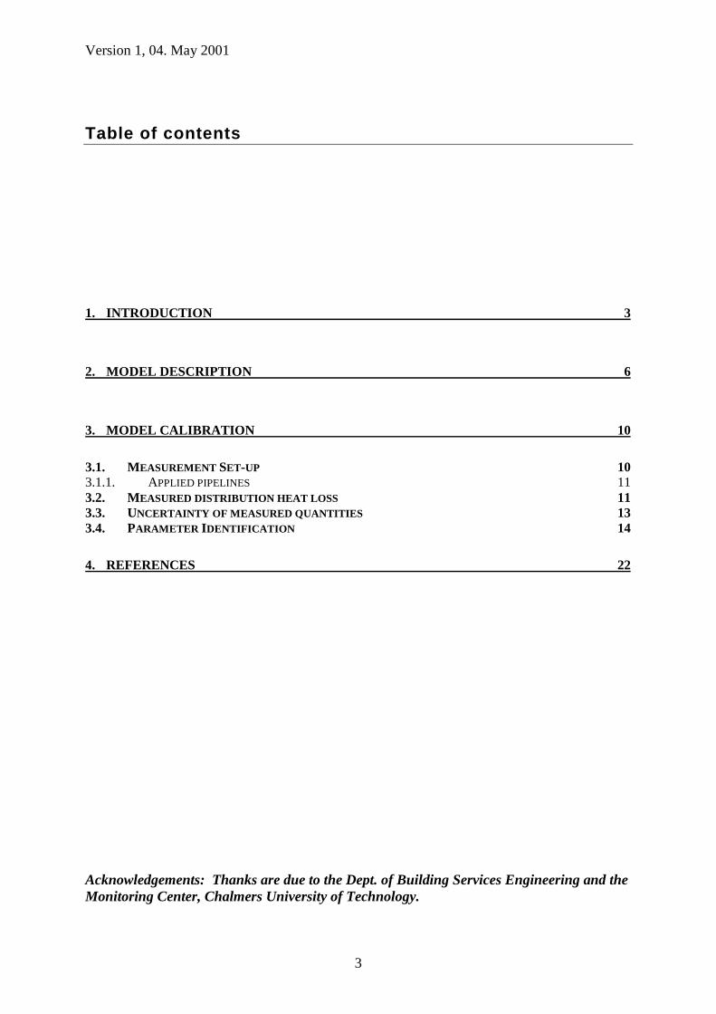
Figure 1.1: Information flow diagram of TYPE 313

Mode 1:In Mode 1 two pipelines in one insulation (twin-pipes) in the ground are modeled. Requiredare physical parameters of the pipe and insulation as well as physical properties of the ground.Parameter 11, the relative length, is multiplied with the length given by parameter 2. Usingthis factor up- and downscaling of a network is possible. For parameter 12 refer to thedescription of the model. The parameter describes an additional heat transfer due to metalspacers between the pipes an inhomogeneous insulation material. The validation proceduredescribed in the following derived a value of 3.3 for this parameter.

Mode 2:In Mode 2 two pipelines (single-pipes) in the ground with separate insulation are modeled.Required are physical parameters of the pipe and insulation as well as physical properties ofthe ground. Parameter 11, the relative length, is multiplied with the length given byparameter 2. Using this factor up- and downscaling of a network is possible. For parameter12 refer to the description of the model. The parameter describes an additional heat transferdue to inhomogeneous insulation material. The recommendation for this parameter in mode 2is 1.0.


6

2. MODEL DESCRIPTION

The standard TRNSYS library offers a pipe model using a user defined UA-value to calculateheat losses dependent on fluid temperature and ambient temperature. This model is notsufficient for calculating ground buried district heating pipelines, since it is not possible toconsider the heat exchange between supply and return pipeline. Especially for small districtheating systems with smaller pipe diameters supply and return pipeline are sharing onecommon insulation. For those pipelines the heat exchange between the two pipelines can notbe neglected. Different work has been done to describe the heat transfer to the ambient andthe heat exchange between the two pipelines, mostly assuming stationary conditions [2].

For dynamic simulation it is not sufficient to consider stationary conditions only. Thepropagation speed of the fluid in the pipeline, dx/dτ, must be taken into account. UsingTRNSYS, the simulation is carried out in predefined time steps and thus, Sections ('plugs') ofdifferent length and volume will proceed inside the pipe. This model type is commonly calledplug-flow model and is used by several different models.

In this work a ground buried plug-flow model was developed, combining the ground buriedpipe model by Wallentén with a plug-flow pipe model. Regarding the modelling of plug-flowthe model is based on the standard TRNSYS Type 31 component. The heat transfer equationsfor the ground buried pipe for stationary conditions are based on analytic equations presentedby Wallentén [13].

Furthermore, Wallenténs equation set was modified by introducing a constant factor, to bemultiplied with the U-value for the heat exchange between two pipes in the ground. Thisfactor accounts for heat bridges and inhomogeneous insulation material over the length of thepipeline.

The principle of the plug-flow pipe simulation model is shown in Figure 2.1.

t1

t1t

i

t3

x x

t

time = i-1τ

time = iτ

L0 0 L

t

t2

t3

t2

Figure 2.1: Principle of the plug-flow simulation model. TRNSYS Type 31.


7

In general, the outlet temperature is calculated:

Equation 2.1:

⋅⋅+⋅

∆⋅= ∑

−

=

1

1τ

1 k

jkkjjo tMatM

mt

ɺ

Where a and k must satisfy:

∑−

=

∆⋅=⋅+

≤≤1

1

τ

10k

jkj mMaM

a

ɺ

Energy losses are considered for each element by solution of the following equation:

)()(τ

envjjpj

pj ttUAd

dtcM −⋅−=⋅

For elements that enter or leave the pipe during a particular time step, only the duration timewithin the pipe is considered. The total energy loss rate to the environment is the summationof the individual losses from each element given as:

Equation 2.2: )()(, envjjpjenvp ttUAQ −⋅=−ɺ

cp = specific heat capacity of fluid [kJ/kg,K]M = mass of fluid [kg]mɺ = mass flow rate of fluid [kg/s]

envpQ −ɺ = energy loss rate from pipe [W]

τ = time [s]t = fluid temperature [°C]to = pipe outlet temperature [°C]UAp = heat loss coefficient [kJ/K]∆τ = simulation time step [s]j,k = refer to segments of fluid in pipe

In this model mixing or conduction between the elements inside the pipe is not considered.The pipe UA-value has to be calculated separately and is given as an input for the simulation.

Wallentén developed calculation models for ground buried pipes. One model describes twosingle pipes in the ground and another model describes two pipes in one insulation (twin-pipe). The models consider the heat exchange between the pipes and calculate the heat loss tothe environment. The principle for both calculation models is shown in Figure 2.2.Difference between the two models are different calculation routines for the U-values.


8

tS ta t1

t0

Symmetrical problem Anti-symmetrical problem Original problem

t00

+ =qS qa -qa q1

Ua(t )2 1-t

qS q2

tS -ta t2

Figure 2.2: Heat loss calculation principle of two pipes in the ground, Wallentén.

The original problem is divided in two part problems. The first part problem is described assymmetrical problem. Here it is assumed that both pipes have the same temperature and thus,no heat exchange between the two pipes occurs. The second part problem is the anti-symmetrical problem. Here, the surface temperature is the average temperature between thetwo pipelines and thus, no heat exchange between the two pipes and the environment occurs.It can be written:

Equation 2.3: ( )

2;

2

:2

2

:

2121

21

021

0

2

1

ttt

ttt

with

ttUtUq

ttt

UttUq

where

qqq

qqq

as

aaaa

SSSS

as

as

−=+=

−⋅=⋅=

−+

⋅=−⋅=

−=+=

t1 = temperature of pipe 1 [°C]t2 = temperature of pipe 2 [°C]t0 = temperature of the ground surface [°C]q1 = heat loss from pipe 1 per meter [W/m]q2 = heat loss from pipe 2 per meter [W/m]qa = heat loss anti-symmetrical problem [W/m]qs = heat loss symmetrical problem [W/m]Ua = heat loss coefficient anti-symmetrical problem [W/m,K]Us = heat loss coefficient symmetrical problem [W/m,K]


9

First order approximations are proposed for the exact solution for calculating the U-values ofboth part problems. The error introduced by the approximation compared to the exactsolution is in within 5%.

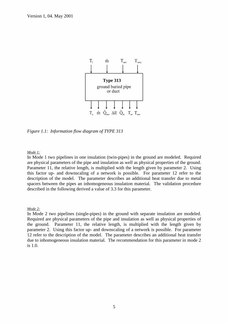
Anyhow, Wallenténs equation set to calculate the U -value for the symmetrical and anti-symmetrical problem is valid for homogeneous insulation and ground materials. Pipelines onthe market usually include metal spacers between the pipelines inside the insulation to keepthe prescribed distance between the pipelines during production. Spacers between thepipelines are heat bridges which increase the pipeline overall value of the anti-symmetricalUa-value. As well, pipe connections and welding seams can increase the pipe overall Ua-value. Therefore a heat transfer factor Fasy was introduced to account for inhomogeneous pipeinsulation material and heat bridges. Thus, qa in Equation 2.3 can be written as:

Equation 2.4: 2

21 ttUFtUFq aasyaaasya

−⋅⋅=⋅⋅=

However, calculating the heat exchange between the pipes for each segment inside the pipethe temperature of the other pipe at the same location has to be known. Here, using the plugflow model introduces difficulties, since usually supply and return pipeline in counter flowhave to be considered. Calculating the heat exchange between the pipes was simplified byusing the average temperature of the counter pipe instead of the exact temperature at the samelocation of the counter section. The heat exchange for each section of each pipe is thus:

Equation 2.5:

2

2

,2,1,21

,2,1,12

javerageaasyj

averagejaasyj

ttUFq

ttUFq

−⋅⋅=

−⋅⋅=

−

−

t1,average = average temperature of pipe 1 [°C]t2,average = average temperature of pipe 2 [°C]t1,j = temperature of segment j in pipe 1 [°C]t2,j = temperature of segment j in pipe 2 [°C]q2-1,j = heat transfer from pipe 2 to segment j of pipe 1[W/m]q1-2,j = heat transfer from pipe 1 to segment j of pipe 2[W/m]

With this simplification the heat transfer from e.g. the hot supply pipe to the cold return pipewill be higher in the beginning of the pipe and lower in the end.

By using Wallenténs model as described Equation 2.2 can be written as:

Equation 2.6: )()()()( ,, averagecounterjjaasyenvjjaasySjenvp ttUFttUFUQ −⋅⋅+−⋅⋅−=−

where tcounter,average is the average temperature of the counter pipeline.


10

3. MODEL CALIBRATION

In this chapter the previous described pipeline model is calibrated using measurements. Themeasurements were carried out for a small district heating network in Tölö, about 30 kmsouth of Göteborg, Sweden. In this residential area a small district heating network isconnected to a larger network via heat exchanger. The small district heating network itself isdivided into three subnets while one is taken out for measurement purposes. In more detail themeasurements are presented in [3].

In this chapter the measurement set-up, the measurements and the calibration of the model arepresented.

3.1. Measurement Set-up

Initially the measurement set-up was designed to obtain the coincidence factor of the networkand separate sections. Anyhow, this set-up also enables a measurement of network heatlosses. In Figure 3.1 the more detailed measured part, net 1, of the larger network is shown.To obtain the coincidence factor one house station, the net 1 and the supply line to theKungsbacka DH network have to be measured. To measure the distribution heat loss of net 1all substations of that route have to be measured.

Many measurement stations and a short sampling interval of 1 minute lead to a large amountof data. Therefore some important measurement points were chosen and only one route, net1, was measured in more detail. One data logger was installed in each of the five housesubstations. Additionally one measurement station was used to record the heat supply to net 1(five houses plus distribution heat losses) and to record the total heat supply for the residentialarea Tölö (20 houses plus two under construction). Figure 3.1 shows the location of themeasurement stations in the network.

Net 1

Net 3

Net 2

Kun

gsba

cka

DH

B

CD

E

F

A

Figure 3.1: Location of data logger stations in the DH network Tölö. A = main substation,B-F = house substations.


11

The main substation is named A while the house stations are numbered from B to F. Eachdata logger station is connected to one computer which operates as measurement computerincluding software and data storage. The measurement computers are not interconnected anddata was transferred frequently from each station separately in periods of about 10 days.

3.1.1. Applied pipelines

The district heating network in Tölö consists of PE mantled steel twin-pipes in three differentsizes from DN50 and DN40 for the main distribution lines and DN25 for the houseconnection pipes. The idea by using twin-pipes (two pipes in one insulation mantle) is alower specific heat loss (W/m) of the distribution line and lower ground costs by decreasingthe width of the route.

Figure 3.2: PE- mantled steel twin-pipe. (picture: PowerPipe)

The route length of net 1 is 170m (DN50: 32m, DN40: 60m, DN25: 78m) taken fromarchitect drawings.

3.2. Measured distribution heat loss

This chapter deals with the heat loss of the distribution network in Tölö. Especially forresidential areas with a low heat density the heat loss of the heat distribution system is ofgreater interest and the distribution heat loss for those areas can be up to 20% of the yearlyheat demand. The Tölö district heating network is, as described, a two pipe network withsupply and return pipe in one common insulation. The largest diameter is DN50 and thesmallest diameter DN25. A two pipe steel network in one common insulation was chosen inorder to minimise the heat loss. The network is equipped with a pipe leakage detection,which is a copper circuit additionally inserted in the insulation in some distance from the steelmantle of the pipe. Using high voltage and measuring the resistance between steel pipe andcopper circuit shows weather the insulation material is moistened or not. The leakage check


12

was performed for all three circuits, net 1 - 3, of the Tölö district heating network and noleakage was detected. Thus, the network heat losses presented here are representing the heatlosses of an undamaged heat distribution system.

With the actual measurement set-up it was possible to determine the distribution system heatloss of net 1. Measuring the flow and return temperature as well as the volume flow of net 1and of each house substation B-F the heat loss can be calculated as an average value from theenergy balance of net 1. The route length of net 1 is 170m in total (DN50: 32m, DN40: 60m,DN25: 78m) whereof about 15% (26m) are bends or T-pieces. As well, about 1 m notinsulated pipes (3.5% of the total) are included in each substation.

In Figure 3.3 the measured specific network heat loss is shown for the average diameter of net1 (DN32) versus the producers data. The measured values are representing average dailyvalues and the applied uncertainty corresponds to the average uncertainty described in chapter3.3. The grey area represents the error introduced by the uncertainty of the total route length,here assumed to be ±10m (170m total route length).

measured pipe heat loss and producer data for NET 1,measured values are based on daily average

02468

1012141618202224

0 5 10 15 20 25 30 35 40 45 50 55 60 65 70 75 80

(TNET1,flow+TNET1,ret) / 2 - Tambient [°C]

spec

ific

heat

loss

[W

/m]

producer data

measured values: ±15%total root length: 176m ±10maverage diameter: ~DN32

Figure 3.3: Heat loss net 1:big black dot = producer data;dots with error bars = measured values based on daily average values;dashed line = measured values assuming constant heat loss coefficient,grey area represents upper and lower limit for the pipeline length of 176m ±10m;black line = producer data assuming constant heat loss coefficient.

The first observation is that all measured values are located in a narrow temperature interval.This is due to the constant flow and as well constant return temperature of the network.Furthermore it can be observed that with given uncertainties of ±15% the network heat loss isabout 20% higher than the producers data for new pipelines. Regarding Jarfelt [8] ageing ofthe insulation material leads to an increase of the thermal conductivity of about 20% over aperiod of 15 to 20 years. This effect is stronger for a CO2 blown pipe insulation as used inTölö compared to CFC blown pipelines. From Fröling [6] it can be learned that small pipesare ageing faster than larger diameters. Fröling shows that for a pipe dimension DN20 anincrease of 10-20% of the thermal conductivity is accomplished after three years. The


13

residential area Tölö and the heat distribution system were built 1996 and were at the time ofthe measurement at an age of three years. Furthermore, it has to be considered that themeasured heat loss also includes insulated pipe connections, not insulated pipes inside thesubstations, T-pieces and wall ducts. The measured distribution heat loss is reasonableregarding these considerations.

3.3. Uncertainty of measured quantities

Using the measurements as presented and in chronological order ([3]) it has to be considered,that the heat losses of a district heating system are small compared to the transferred energy aswell as the volume flow in the pipe is relatively high. In turn, the temperature drop of theflow pipeline is at its most about 2grC from main station to the substation. Therefore it isnecessary, to evaluate measurement uncertainties more accurate.

Here, the measurement uncertainty is evaluated according to the recommendations given bythe International Organisation for Standardisation, [7], [10], [12]. Here the general statementis made that 'In general, the result of a measurement is only an approximation or estimate ofthe value of the specific quantity subject to measurement that is, the measurand, and thus theresult is complete only when accompanied by a quantitative statement of its uncertainty'.Two terms are used to describe two types of uncertainty. 'Type A' uncertainty is used foruncertainties due to random effects. Evaluation of this type of uncertainty can be treated bystatistical methods. 'Type B' uncertainty includes all uncertainties which are not of 'Type A',commonly so called systematic errors. Type B uncertainties can only be evaluated byexperience and knowledge about the experimental set-up.

The measured data from Tölö includes Type A and Type B uncertainties. The instrumentuncertainty is presented as combined Type A and Type B uncertainty. Here, the instrumentuncertainty is due to random effects, including the Type A and B uncertainties for calibration,meter reading and operating conditions. To evaluate Type B uncertainties, i.e. for installation,knowledge about the measurement set-up and physical conditions is necessary. Therefore,this type of uncertainty is evaluated in more detail and corrections to compensate these effectsare proposed. Finally, combined uncertainties for calculated quantities such as power andenergy are calculated and presented.


14

In general uncertainties can be combined in three ways: 1. uncertainties are added, 2.uncertainties are taking out each other or 3. combined using a statistical compromise. Method1. produces usually too high and method 2. too low uncertainties. A statistical compromiseresults to uncertainties somewhere in between method one and two. In this study, the socalled "law of propagation of uncertainty" or as well called "root-sum-of-squares" is used todescribe combined uncertainties. It is presumed that the measured parameters are notcorrelated. Thus, all uncertainties have been combined as:

Equation 3.1 ( ) ( )∑=

∂∂=

N

ii

ic xu

x

fyu

1

2

2

2

where:

uc(y) = combined uncertainty

N = number of specific standard uncertainties

u(xi) = standard uncertainty associated with input estimate xi

In the following all combined uncertainties are given for a confidence level of 68%, whichcorresponds to a coverage factor of k=1.

3.4. Parameter Identification

The district heating circuit model consists of twin-pipe models as described in 3.1.1. Tocalibrate the model for the heat distribution two requirements have to be met: the calculateddistribution heat losses and distribution temperatures have to be in agreement with themeasured values.

For calibration the net 1 flow temperature and volume flow and the house substation volumeflow and power were provided as an input for the simulation. The measured ambienttemperature was taken as an input to calculate the pipe heat losses. The simulation wascarried out using a time step of one minute.

Using these inputs for simulation the model calculates the flow temperature for each housesubstation taking heat losses and heat transfer between the supply and return pipeline intoaccount. Together with the house substation power as an input the house substation returntemperature can be calculated. Again calculating distribution heat losses and heat transferbetween the pipelines the net 1 return temperature is calculated. The model is taken as beingcalibrated when the calculated distribution heat loss is in best agreement with themeasurement and the difference between measured and calculated return temperature issmallest. The principle of the heat distribution model for Tölö is shown in Figure 3.4.


16

Measured DATA

DF - dynamic fitting

Pm - Pc

new parameter values

dynamic fitting procedure

parameter set to identify

update parameter set

Pm (,Tm)

Pc (,Tc)TRNSYS DH network model

temperature and flow net 1, ambient temperature, house substation power and flow

Best fitting parametervalues

Figure 3.5: Heat distribution pipe parameter identification using TRNSYS and DF.

Fixed inputs for each pipe component are the geometrical properties of the pipe dimension,the heat conductivity of the ground and the fluid properties of the water in the pipe.Parameters free for identification were the pipe insulation heat conductivity and heat transferfactor for the heat exchange between the supply and return pipeline. As an example the pipeparameters are shown in

Table 3.1 for the first pipe section of net 1, using a DN50 twin-pipe.


17

Table 3.1: Important parameters for first pipe section of net 1, DN50 twin-pipe.

No. Description Value Unit

1 Operation mode:1 = calculating ground temperature2 = Type 31 original mode3 = twin-pipe in the ground4 = single pipe in the ground after Wallentén

3 -

2 Pipe length 31.6 m

3 Pipe inside diameter 0.0603 m

4 Pipe outside diameter 0.2 m

5 Pipe depth in the ground(surface - pipe centre)

0.6 m

6 Specific heat capacity of the fluid 4.18 kJ/kg,K

7 Density of the fluid 988 kg/m3

8 Thermal conductivity of the pipe insulation,λiso

to beidentified

W/m,K

9 Thermal conductivity of the ground 1.5 W/m,K

10 Initial temperature of the fluid 60 °C

11 Relative pipe length 1 -

12 Heat transfer factor used for asymmetricalheat transfer coefficient, Fasy

to beidentified

-

13 Distance between pipe centres 0.0803 m

Italic letters are set values specific for each pipe dimension and are taken from the producersdata sheet. Bold letters are values to be identified. Normal letters are general parametervalues set and used for all pipe dimensions.

The parameter identification procedure was carried out in two steps: First the parameter valuefor the pipe insulation heat conductivity was identified by comparing measured and calculatedpipe heat loss. The transfer factor was set to a value of 1 which represents Wallenténsequation set in its original version. Second, using the best fitting pipe insulation heatconductivity from step one as an input the heat transfer factor was identified by comparing thesum of measured and calculated net 1 and house return temperatures.

In Table 3.2 the result of the parameter identification of step one is presented for the first andthe second measured data period. The objective represents the average difference between themeasured and calculated heat loss of the distribution system of net 1. The shaded cell for thefirst data period represents the objective using the identified thermal conductivity from dataperiod two. Vice versa for the second data period.


18

Table 3.2: Identification of thermal conductivity of pipe insulation material using first andsecond measured data period. Objective = average difference between measuredand calculated heat loss of net 1.

λiso [W/m,K] objective [kW] objective [kW]

1st data period 0.033 ± 0.001 2.51 2.53

2nd data period 0.038 ± 0.001 2.10 2.12

The outcome of the identification is a similar result for both runs. Anyhow, it can be seen thatthe thermal conductivity is somewhat higher for the second period with a lower objective.The objective of 2.1 or 2.5 kW can not be related to the average yearly heat loss of net 1 butto the average difference between supplied energy to net 1 and the actual total demand of thehouse substations of 8.3 kW on a minute basis. Due to the large amount of data the absoluteerror by identifying the thermal conductivity is little.

To provide a value for the thermal conductivity of the pipe insulation of net 1 the identifiedvalues were weighted related to the length of the measured data period. The value of 0.036W/m,K was used as an input to identify the heat transfer factor for the heat exchange betweenthe supply and return pipeline. The objective here represents the average difference betweenthe sum of measured and calculated return temperatures of net 1 and all house substations.

Table 3.3: Identification of heat transfer factor using first and second measured data period.Objective = average difference between the sum of measured and calculatedreturn temperatures.

Fasy [-] objective [°C] objective [°C]

1st data period 3.7 ± 0.5 5.6 5.7

2nd data period 2.9 ± 0.4 6.9 7.1

The result is similar for the two data periods, especially with regard to the absolute error bydetermining the heat transfer factor. The heat transfer factor for the two periods is weightedby the length of the periods and the value of Fasy = 3.3 is taken for further investigations. Itcan be noted that the objective for the first period using a heat transfer factor of 1.0, i.e. usingthe equation set as originally proposed by Wallentén, is 8.1°C. This shows the necessity ofthe heat transfer factor, which can be explained by steel spacers welded between supply andreturn pipeline, which is not considered in the original equation set. Regarding a 12 mdistribution pipeline a heat transfer factor of 3.3 would correspond to about 25cm steelspacers between supply and return pipeline (λiso=0.036 W/m,K; λsteel=45 W/m,K).

In Table 3.4 the measured and calculated net 1 distribution heat loss is presented using aheat conductivity of the insulation material of 0.036 W/m,K and a heat transfer factor of3.3.


19

Table 3.4: Measured and calculated net 1 heat loss for period 1, 2 and all measurementsused for net 1 simulation model calibration.

measured heat loss[kWh]

calculated heat loss[kWh]

difference[%]

Period 1 -379 -398 4.9

Period 2 -627 -599 -4.8

Total -1 878 -1 822 -3.1

The difference is less than 5% for all presented periods. In Figure 3.6 the measured andcalculated heat loss and the difference are shown on a daily basis. The maximum recordeddifference is about 30%. It can be seen that the difference is higher than for the periods intotal.

-80

-60

-40

-20

0

20

40

60

80

26-fe

b-99

28-fe

b-99

02-m

ar-9

9

04-m

ar-9

9

06-m

ar-9

9

08-m

ar-9

9

10-m

ar-9

9

12-m

ar-9

9

14-m

ar-9

9

16-m

ar-9

9

18-m

ar-9

9

20-m

ar-9

9

22-m

ar-9

9

24-m

ar-9

9

26-m

ar-9

9

28-m

ar-9

9

30-m

ar-9

9

01-a

pr-9

9

net 1

hea

t los

s [k

Wh/

day]

-40

-30

-20

-10

0

10

20

30

40

diffe

renc

e [%

]

period 1 period 2difference

calculated

measured

Figure 3.6: Measured an calculated net 1 distribution heat loss and difference on a dailybasis.

Anyhow, it could be shown that by comparing longer periods the difference betweenmeasured and calculated heat loss decreases and the influence of the ground and pipecapacitance is less important. To evaluate the distribution heat loss on a yearly basis themodel is taken as being calibrated regarding heat losses.


20

The second criteria to calibrate the calculation model of net 1 are the measured and calculatedhouse substation flow temperatures and the net 1 return temperature. In addition to calibratethe model for heat losses the model was calibrated for temperatures. In Figure 3.7 themeasured and calculated house flow and return temperatures for the building closest (houseB) and the building furthest (house F) from the main substation are shown for 12 hours, basedon minute values.

0

10

20

30

40

50

60

70

12:00 13:00 14:00 15:00 16:00 17:00 18:00 19:00 20:00 21:00 22:00 23:00

time 22. March 1999

tem

pera

ture

[°C

] ThouseF,flow

Tnet1,flow

thin lines: calculatedthick lines: measured

ThouseB,flow

Tnet1,ret

Figure 3.7: Measured and calculated house substation flow temperatures and net 1 flow andreturn temperature for the second half of the 22. March 1999, based on minutevalues.

It can be seen that the calculated temperatures are in the same range as the measured values.The measured temperature curve is slightly smoother than the calculated curve which can beexplained by capacitance effects of the pipeline and ground which are not taken into accountby the simulation model. Figure 3.8 shows the measured and calculated return temperature ofnet 1 for one hour based on minute values.


21

0

10

20

30

40

50

60

70

23:00 23:15 23:30 23:45time 22. March 1999

tem

pera

ture

[°C

]

ThouseF,flow

Tnet1,flow

thin lines: calculatedthick lines: measured

ThouseB,flow

Tnet1,ret

Figure 3.8: Measured and calculated house substation flow temperatures and net 1 flow andreturn temperature for one hour, based on minute values.

It can be seen that the calculated return temperature is higher than the measured returntemperature most of the time. This indicates a slightly higher heat transfer from the supply tothe return pipeline. A better fit of measured and calculated return temperature of net 1 couldhave been obtained by another choice of objective. Here, the sum of temperature differencesbetween all measured and calculated house substation flow temperatures and the measuredand calculated net 1 return temperature was taken to identify the heat transfer factor. Usingthis objective all temperature differences were valued equally and thus, more weight is put onfitting the house substation flow temperatures.


22

4. REFERENCES

[1] Boverket (1991): Byggvägledning 10 - Vatten och Avlopp (Building guidelines - watersupply and sewer), En handbok I anslutning till nybyggnadsregler NR.

[2] BØhm, B. (1999): Heat Losses from Buried District Heating Pipelines, DoctoralThesis, Technical University of Denmark, Denmark.

[3] Dahm, J. (1999): Small District Heating Systems, Doctoral Thesis, DocumentD48:1999, Dept. of Building Services Engineering, Chalmers University of Technology,Sweden.

[4] Dahm, J. (1998): Small Central Solar Heating Systems: Measurements - SimulationModel Validation - Evaluation, Proceedings ACEEE's 1998 Summer Study on EnergyEfficiency in Buildings, Monterey CA, USA.

[5] Dahm, J.; Bales, C.; Lorenz, K.; Dalenbäck, J.-O. (1998): Evaluation of StorageConfigurations with Internal Heat Exchangers, Solar Energy, Vol. 62, No. 6, p. 407-417.

[6] Fröling, M., Jarfelt, U., Ramnäs, O. (1999): Insulation of district heating pipes -Environmental aspects of the blowing agent of polyurethane foam, Proceedings of the7th International Symposium on District Heating and Cooling, Nordic Energy and ResearchProgramme, Lund, Sweden.

[7] International Organization for Standardization (1993): Guide to the Expression ofUncertainty in Measurement, first editon 1993, ISBN 92-67-10188-9, Switzerland.

[8] Jarfelt, U. (1999): Changes in thermal conductivity of district heating pipes. Fieldstudy, Proceedings of the 7th International Symposium on District Heating and Cooling,Nordic Energy and Research Programme, Lund, Sweden.

[9] Lindskog, J. (1994): Mätvärdesbehandling och rapportering av mätresultat (TreatingMeasurements and Presenting the Results), Sandtorp Consult AB, Hjo, Sweden, ISBN 91-972122-8-8. In Swedish.

[10] Taylor, B.N., Kuyatt, Ch.E. (1994): NIST Technical Note 1297, Guidelines forEvaluating and Expressing the Uncertainty of NIST Measurement Results, USDepartment of Commerce Technology Administration, Nat. Institute of Standards andTechnology, USA.

[11] Spirkl, W. (1995): InSitu Scientific Software: DF - Dynamic System Testing, programmanual.

[12] Taylor, B.N., Kuyatt, C.E. (1994): Guidelines for Evaluating and Expressing theUncertainty of NIST Measurement Results, NIST Technical Note 1297, 1994 Edition,United States Department of Commerce, National Institute of Standards and Technology,USA.

[13] Wallentén, P. (1991): Steady State Heat Loss from Insulated Pipes; LicentiateThesis, Report TVBH-3017, Dept. of Building Physics, Lund Institute of Technology,Sweden.

Date post:	01-Apr-2018
Category:	Documents
Upload:	dangdat
View:	219 times
Download:	1 times

District Heating Pipelines in the Ground - Simulation Model · District Heating Pipelines in the...

Documents