Discussion PaPer series

IZA DP No. 10863

Wang-Sheng LeeTerra McKinnish

The Marital Satisfaction ofDifferently-Aged Couples

juNe 2017

Any opinions expressed in this paper are those of the author(s) and not those of IZA. Research published in this series may include views on policy, but IZA takes no institutional policy positions. The IZA research network is committed to the IZA Guiding Principles of Research Integrity.The IZA Institute of Labor Economics is an independent economic research institute that conducts research in labor economics and offers evidence-based policy advice on labor market issues. Supported by the Deutsche Post Foundation, IZA runs the world’s largest network of economists, whose research aims to provide answers to the global labor market challenges of our time. Our key objective is to build bridges between academic research, policymakers and society.IZA Discussion Papers often represent preliminary work and are circulated to encourage discussion. Citation of such a paper should account for its provisional character. A revised version may be available directly from the author.

Schaumburg-Lippe-Straße 5–953113 Bonn, Germany

Phone: +49-228-3894-0Email: publications@iza.org www.iza.org

IZA – Institute of Labor Economics

Discussion PaPer series

IZA DP No. 10863

The Marital Satisfaction ofDifferently-Aged Couples

juNe 2017

Wang-Sheng LeeDeakin University and IZA

Terra McKinnishUniversity of Colorado and IZA

AbstrAct

juNe 2017IZA DP No. 10863

The Marital Satisfaction ofDifferently-Aged Couples*

We investigate how the marital age gap affects the evolution of marital satisfaction over

the duration of marriage using household panel data from Australia. We find that men tend

to be more satisfied with younger wives and less satisfied with older wives. Interestingly,

women likewise tend to be more satisfied with younger husbands and less satisfied with

older husbands. Marital satisfaction declines with marital duration for both men and

women in differently-aged couples relative to those in similarly-aged couples. These relative

declines erase the initial higher levels of marital satisfaction experienced by men married to

younger wives and women married to younger husbands within 6 to 10 years of marriage.

A possible mechanism is that differently-aged couples are less resilient to negative shocks

compared to similarly-aged couples, which we find some supportive evidence for.

JEL Classification: D1, J12

Keywords: assortative matching, marital age gap, marital duration, marital satisfaction

Corresponding author:Wang-Sheng LeeDepartment of EconomicsDeakin University70 Elgar RoadBurwood, Victoria 3125Australia

E-mail: wang.lee@deakin.edu.au

* We are grateful to two anonymous referees for providing very helpful comments and suggestions. This paper uses unit record data from the Household, Income and Labour Dynamics in Australia (HILDA) Survey. The HILDA Project was initiated and is funded by the Australian Government Department of Social Services (DSS) and is managed by the Melbourne Institute of Applied Economic and Social Research (Melbourne Institute). The findings and views reported in this paper, however, are those of the author and should not be attributed to either DSS or the Melbourne Institute.

  1

I. Introduction

A well-documented feature of the marriage market is that individuals match assortatively

on age and that the most common pairing is one in which the husband is a few years older than

the wife (Presser, 1975; Glick and Lin, 1986). While this pattern of matching on age is well-

known, the underlying mechanism that generates this sorting is not well understood. For

example, some studies suggest that marital gains are largest in older husband-younger wife pairs

(Bergstrom and Bagnoli, 1993) while others find that marital gains are largest for similarly-aged

couples (Choo and Siow, 2006). A number of theoretical models assume that men (and in some

models, women) prefer younger spouses for their “fitness” or fecundity (Siow, 1998; Coles and

Francesconi, 2011; Diaz-Gimenez and Giolito, 2013), while analysis using online and speed

dating data suggest that both men and women instead prefer similarly-aged partners (Belot and

Francesconi, 2013, Hitsch, Hortascu and Ariely, 2010).

Marital sorting is an outcome of both male and female preferences as well as the

distribution of characteristics in an individual’s marriage market. Assortative matching on age

can occur if both men and women prefer similarly-aged spouses, but this same pattern of sorting

can also result from underlying preferences in which both men and women prefer younger

spouses. Women could, for example, prefer to match with younger men, but if most men receive

large disutility from marrying an older woman, women will avoid seeking younger male

partners.

This paper adds to the existing literature by analyzing how marital satisfaction varies

with the marital age gap. Specifically, this paper analyzes data from the 2001-2013 waves of the

Household, Income and Labor Dynamics in Australia (HILDA) data. These longitudinal data are

particularly well-suited to this study as they contain annual reports of satisfaction with

relationship with one’s current spouse from both the husband and the wife. Determining whether

  2

marital satisfaction is greater for similarly-aged couples, for men and women married to younger

spouses, or for both men and women in older husband-younger wife pairings will provide insight

regarding the conflicting assumptions and results from previous theoretical and empirical

research on marital sorting by age.

In addition to studying the cross-sectional relationship between the marital age gap and

marital satisfaction, ours is the first study to analyze how the marital age gap affects the

evolution of marital satisfaction over the duration of the marriage. Because we observe annual

reports of marital satisfaction we are able to control for individual fixed-effects in our analysis.

Unlike analysis that compares recently-married couples to couples with longer marital duration,

this fixed-effects analysis is identified using within-marriage changes in marital satisfaction over

time. We are therefore able to ascertain whether marital satisfaction evolves differently over the

duration of the marriage for differently-aged couples compared to similarly-aged couples. For

example, if men married to younger wives initially express greater marital satisfaction, does this

higher level of marital satisfaction persist, increase or decrease over the duration of the

marriage?

Research on marital dissolution has found that differently-aged couples are more likely to

divorce than similarly-aged ones (Cherlin, 1977; Lillard et al, 1995), which suggests that

differently-aged couples may experience greater declines in marital satisfaction over time.

Previous work suggests that unanticipated shocks to marital gains are a key cause of marital

dissolution (Becker, Landes and Michael, 1977; Weiss and Willis, 1997). Therefore, if our

analysis finds that marital satisfaction declines over time for differently-aged couples relative to

similarly-aged couples, a potential mechanism is that differently-aged couples suffer larger

losses to marital gains when experiencing a negative shock. This could happen if, for example,

differently-aged couples are less similar in their preferences for consumption, making it more

  3

difficult for them to adjust to a negative economic shock. Fortunately, the HILDA data include

self-reports of whether there was a “major worsening of finances” in the past year, which allows

us to test this mechanism.

Our key findings are: 1) Men tend to be more satisfied with younger wives and less

satisfied with older wives. 2) Likewise, women tend to be more satisfied with younger husbands

and less satisfied with older husbands. 3) For both men and women, marital satisfaction declines

over the duration of the marriage for those married to differently-aged partners relative to those

married to similarly-aged partners. These relative declines erase the initial higher levels of

marital satisfaction experienced by men married to younger wives and women married to

younger husbands within 6 to 10 years of marriage. 4) Differently-aged couples experience

larger declines in marital satisfaction in response to a negative economic shock compared to

similarly-aged couples.

II. Literature and Background

A. Theoretical models of marital sorting and marital age gap

Several theoretical papers in economics focus on the gender differences in timing of

marriage or the age gap between partners. Predictions from these papers regarding the

relationship between the marital age gap and marital gains are driven by assumptions regarding

individual preferences for partner characteristics and the evolution of earnings and/or fecundity

over the lifecycle.1

                                                            1 In the discussion below, we assume that individual reports of marital satisfaction are a proxy for the marital gains they experience. It should be noted that we implicitly assume that marital search is costly. If it were the case that individuals search at very low cost in large marriage markets with no gender imbalances, we would expect for competition among prospective mates to compete away any excess marital gains so that all couples begin marriage with equivalent (and zero) gains relative to their outside alternative (Weiss and Willis, 1997). Given that even among recently-married couples there is considerable variation in marital satisfaction, this seems a reasonable assumption.

  4

Bergstrom and Bagnoli (1993) assume that husband quality is revealed at later ages than

wife quality. This happens when marital gains come from household specialization, and men’s

market productivity increases over time but women’s household productivity does not. All

women marry young, because delays in marriage do not increase their value on the marriage

market. High quality women marry high quality older men who have delayed marriage to reveal

their high earnings potential. Low quality young women marry low quality young men, who do

not bother to delay marriage because their earnings potential will not improve over time.

The Bergstrom and Bagnoli model predicts that differently-aged couples contain matches

of high quality husbands and wives, generating greater surplus, while similarly-aged couples

contain lower quality husbands and wives with lower surplus. This predicts greater marital

satisfaction for both men and women in older husband-younger wife couples compared to

similarly-aged couples.

Coles and Francesconi (2011) assume that both men and women receive utility from their

partner’s income but also from their partner’s “fitness”, which decays with age. Financially

successful men and women are both able to attract younger spouses. The younger partners

receive disutility from matching with an older spouse, but are compensated by the higher

earnings of the older spouse. Unlike Bergstrom and Bagnoli (1993), it is not clear that the

younger spouses in large age gap couples will be more satisfied than one in a small age gap

couple. The younger spouse has traded off one feature (household income) for another (partner

"fitness").2 We would expect the relationship between marital age gap and marital satisfaction to

be sensitive to controls for partner characteristics, such as education and income.

                                                            2 Siow (1998) generates a very similar prediction: that older husband-younger wife pairs are generated because financially successful older men prefer younger “fecund” women, and compensate their younger partners for marrying them with higher earnings. His model, however, does not result in older wife-younger husband pairings because he assumes that only young women are fecund and all women marry young in order to produce children.

  5

Both Bergstrom and Bagnoli (1993) and Coles and Francesconi (2011) predict that in

couples with large age gaps the older spouse is financially successful. Mansour and McKinnish

(2014), however, find empirically that both members of differently-aged couples tend to be

negatively selected on education, earnings and cognitive ability. This calls into question whether

these theoretical models are realistic descriptions of the process that generates differently-aged

couples.3

Diaz-Gimenez and Giolito (2013) develop a model in which older husband-younger wife

pairs are generated simply because fecundity declines more rapidly for women than men over the

lifecycle. Women prefer to marry young, while still fecund, and are willing to accept marriage

proposals from older men, whose fecundity declines at a slower rate. In contrast, it is less costly

for men to delay marriage and they reject proposals from less-fecund older women. Their results

imply that men should receive greater disutility from an older spouse than women, given

women’s more rapidly declining fertility.

It should be noted that the theoretical papers on marital sorting discussed in this section

generate predictions regarding the formation of couples, but do not provide any insight regarding

how marital gains evolve over time inside marriage.

B. Revealed preference and marital age gaps

While there is no empirical research that directly analyzes individual’s preferences for

marital age gaps, the relevant empirical research is consistent with preferences for similarly-aged

spouses, with a preference for pairings with slightly older husbands compared to slightly older

wives. For example, Choo and Siow (2006) develop and estimate a structural model of the

                                                            3 Mansour and McKinnish argue that their empirical results likely reflect the fact that men and women with higher earnings potential spend more time in age-homogenous settings (e.g. postsecondary and graduate education, jobs with career ladders) and therefore are more likely to marry similarly-aged spouses.

  6

marriage market. They estimate systematic net gains to marriage based on age of husband and

wife, and find that women maximize their net gain with a slightly older husband and men

maximize their net gain with slightly younger wives. These larger estimated gains to marriage

for slightly older husband-slightly younger wives pairings are generated by the fact that these

pairings are the most common, conditional on the distribution of available partners in the market.

Belot and Francesconi (2013) analyze data from speed-dating events and find that both

men and women prefer dates where the man is 0-5 years older rather than dates where the man is

more than 5 years older or where the man is younger than the woman. Using online dating data,

Hitsch, Hortacsu and Ariely (2010) find that both men and women are more likely to contact

similarly-aged partners. Their estimates also indicate that both men and women particularly

avoid pairings in which the woman is older than the man. In the absence of strategic behavior,

these results suggest that preferences for age difference match the empirically observed age

differences at marriage.4

But these studies only reveal true preferences if individuals are not acting strategically

(Fisman et al., 2006). If men or women avoid contacting much younger potential partners

because they suspect the chance of success is very low, this will make it appear as if they prefer

similarly-aged spouses more than they actually do. Therefore, the fact individuals are more likely

to contact, date and marry similarly-aged partners could be generated by preferences for

similarly-aged partners, but this sorting could also be generated by the case in which both men

and women prefer younger spouses.

                                                            4 Hitsch et al (2010) investigate for evidence of strategic behavior using appearance ratings. They find that for both men and women, regardless of appearance rating, the probability of emailing a potential dating partner is monotonically increasing in the attractiveness of the potential partner. There is no evidence, for example, that less attractive individuals strategically avoid contacting the most attractive potential partners. Based on these, Hitsch et al (2010) conclude that there is little evidence of strategic behavior, although they acknowledge that they are only considering one characteristic: physical appearance.

  7

Studying how marital satisfaction varies with marital age gap therefore complements the

existing literature on marital age gap preferences. There is no reason to believe that strategic

behavior plays a role in how people report their marital satisfaction. Therefore, if we find that

married individuals report greater satisfaction when married to similarly-aged partners; this

would be consistent with previous findings that individuals prefer to date and marry similarly-

aged partners. Alternatively, if we find that individuals report greater marital satisfaction when

married to younger spouses, this suggests that the prior findings may in part have been generated

by strategic behavior.

There is limited prior research estimating the relationship between marital age gaps and

marital satisfaction. Using cross-sectional data from Florida in the early 1970s, Vera et al. (1985)

find no significant differences in marital quality among couples from various age gap categories.

Their null result may stem from the fact that husbands and wives were pooled into the same

regression.5 Rogler and Procidano (1989) also find no evidence that marital quality varies with

the marital age gap in their analysis of 200 Puerto Rican families in New York City.

Alternatively, Groot and Van Den Brink (1998) find that both men and women report greater life

satisfaction if there is a positive age gap between husband and wife, but they do not study marital

satisfaction. Their sample is fairly different from ours, as theirs is a sample of older Dutch

couples in which the head of household is ages 43-65, and they also fail to control for marital

duration.6 Finally, Zhang et al. (2012) find in a cross-sectional sample of Hong Kong couples

that husbands two to four years older than their wives were 1.92 times more likely to be satisfied

with their marriages compared with those whose wives were of a similar age to themselves. The

                                                            5 In other words, if husbands are happier in older husband-younger wife marriages than marriages without an age gap, but wives are less happy in older husband-younger wife marriages than marriages without an age gap, this can average out to no effect of age gap on marital satisfaction if husbands and wives are pooled together. 6 Another paper which studies the outcomes of older married couples as a function of the marital age gap is Drefahl (2010), who finds that in a sample of danish individuals over 50, having an older spouse increases the mortality rate for both men and women, and having an older spouse increases the mortality rate for women.

  8

Zhang et al. study, however, controls for both husband’s and wife’s age in addition to their set of

age difference categories. Because simultaneously controlling for both husband’s and wife’s age

controls for any linear effect of age difference, their coefficient estimates for the age difference

categories are difficult to interpret, only reflecting non-linear effects conditional on any linear

effect.

C. Marital duration, marital age gaps and marital satisfaction

There are no studies we are aware of that examine from either a theoretical or empirical

perspective how the marital age gap affects the evolution of marital satisfaction over the duration

of the marriage. Prior work by economists argues that couples marry with imperfect information

and unanticipated shocks can cause gains to marriage to change in ways that were not predictable

at the time of the marriage (Becker, Landes and Michael, 1977; Weiss and Willis, 1997). The

marital age gap could therefore affect changes in marital satisfaction over time by influencing

how unanticipated shocks affect the gains from the marriage.

For example, if similarly-aged couples are more similar in their preferences for

consumption, they might be better able to adjust to a negative financial shock than a differently-

aged couple. If differently-aged couples engage in more household specialization, they might be

more negatively affected by a health shock (because the spouses are poor substitutes for each

other in both market and household production). It should be acknowledged, however, that if

this larger negative effect of the shock on the differently-aged couple causes divorce, an analysis

of marital satisfaction using the selected sample of surviving couples will underestimate this

effect.

In our analysis, we first test whether the evolution of marital satisfaction over the

duration of the marriage is affected by the marital age gap. We also allow the degree of

  9

household specialization to affect trends in marital satisfaction. Finally, we test whether the

effect of negative financial shocks and health shocks on martial satisfaction differs for

differently-aged couples compared to similarly-aged couples.7

III. Data and Methods

A. Analysis sample

This analysis uses the Household, Income and Labor Dynamics in Australia (HILDA)

survey data for the years 2001-2013. The HILDA is a household-based panel study which began

in 2001 with a nationally-representative sample of Australian households in private dwellings.

The initial wave surveyed 7,682 households containing 19,914 individuals, who have then been

re-surveyed annually. In each survey year, all current household members of these initial wave 1

respondents are included in the survey.

One feature of the HILDA survey is that each year it asks respondents to report life

satisfaction on a variety of dimensions, including reporting level of satisfaction with relationship

with partner on a scale from 0 to 10. Therefore, these HILDA data are unusually rich in that they

provide, for a large representative sample, annual reports of relationship quality made by both

members of the couple for as many as to 13 years in a row.

Our analysis sample contains observations in which: 1) both members of the couple

report that they are currently married, 2) both are in their first marriage and 3) both members are

ages 20-55.8

                                                            7 Another form of unanticipated shock to a marriage can be a shock to one’s outside alternatives. If there is a shock that changes a married individual’s perception of the average quality of his or her alternative mates, this will likely also affect their reported satisfaction with their current marriage. We cannot observe these shocks empirically and don’t have any a priori reasoning for why the effect of such shocks should differ by marital age gap. 8 Although the paper does not focus on cohabitating couples, cohabitation is relatively common in Australia and often precedes marriage. In 2010, almost eight in ten (79%) marriages were preceded by a period of cohabitation (Australian Bureau of Statistics, 2012). Selection into marriage from cohabitation (or more broadly selection into marriage from dating) does mean that results might differ if we were studying couples from their first date or from

  10

The independent variable of interest is the within-couple age difference:

AgeDiff = Husband’s Age – Wife’s Age

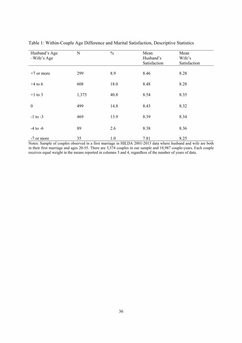
Table 1 reports descriptive statistics for our analysis sample. For Table 1, the sample is divided

based on AgeDiff into 7 categories: +7 or more, +4 to 6, +1 to 3, 0, -1 to -3, -4 to -6, and -7 or

more. Columns 1 and 2 report frequencies and percentages for the distribution of AgeDiff. As

has been previously well-documented, most married couples have a husband who is 0 to 3 years

older than the wife (55.6%). While it is somewhat common to have a husband who is at least 7

years older than the wife (8.9%), it is relatively uncommon for the wife to be 4 or more years

older than the husband (3.6%).

Columns 3 and 4 of Table 1 report the mean reported satisfaction level of husbands and

wives by age difference category. The sample means indicate that on average husbands report

greater satisfaction than their wives. This is consistent with previous studies of marital

satisfaction which have found that wives’ reports of marital satisfaction are significantly lower

than husbands’. For example, national surveys of married adults in the United States in 1980 and

2000 found that, on average, women reported lower levels of marital quality (Amato et al.,

2007).

Men with wives who are at least 7 years older report the lowest levels of satisfaction, and

satisfaction increases monotonically as husband’s age increases relative to wife’s, up until the

husband is more than 3 years older than the wife. For women, the relationship between marital

satisfaction and age-difference with spouse is less obvious from the raw means.

                                                                                                                                                                                                the start of cohabitation, but should not threaten our interpretation of our results as conditional on entry into marriage. 

  11

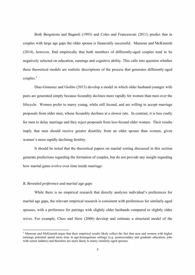
Figure 1 plots male marital satisfaction by marital age gap and marital duration

conditional on male age and age-squared.9 This descriptive plot improves upon the raw means

reported in Table 1 in two ways. First, it is important to control for age when analyzing the

relationship between marital age gap and marital satisfaction. On average, men married to

younger wives enter the analysis sample at older ages and men married to older wives enter the

sample at younger ages. Older individuals report lower marital satisfaction on average, even

conditional on marital duration. Therefore, the lower average levels of marital satisfaction

reported in Table 1 for men married to younger wives may be due to the fact that these men are

older, rather than the fact that they are married to younger wives. Second, Figure 1 takes into

account the fact that marital satisfaction varies with marital duration, and the relationship

between the marital age gap and marital satisfaction may also change over time.

Using Figure 1 to look at men in relatively new marriages (5 years or less), there is a

clear monotonic relationship between the marital age gap and husband’s satisfaction, where men

with much younger wives are the most satisfied and men with much older wives are the least

satisfied. Figure 1 also shows that the relationship between the marital age gap and marital

satisfaction changes with marital duration because marital satisfaction declines more rapidly for

men with larger marital age gaps, and the decline is particularly steep for men with much

younger wives. For men married 6 years or more, husbands married to moderately younger

wives report the highest average levels of satisfaction.10

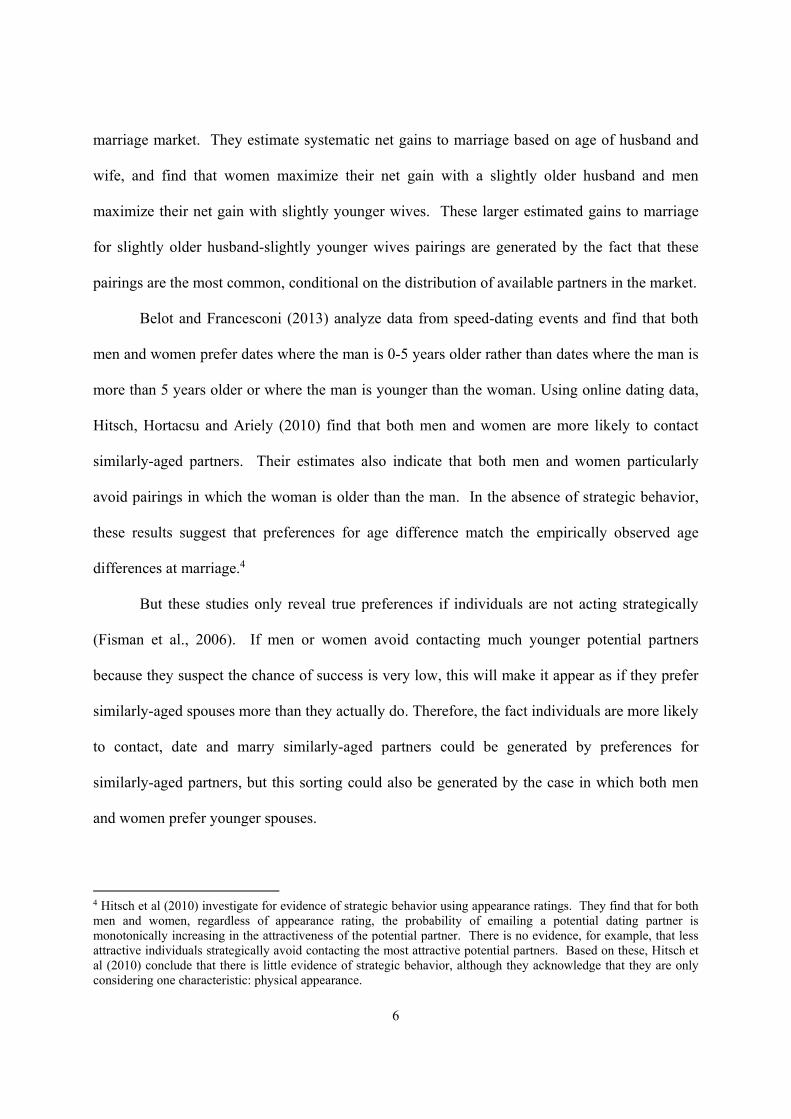
Figure 2 is the analogous plot for wife’s marital satisfaction, this time conditional on the

wife’s age and age-squared. Looking at women in relatively new marriages, the plot shows that

                                                            9 Specifically, Figure 1 is a bivariate smooth function that estimates male marital satisfaction for different combinations of the marital age gap and marital duration by tensor product P-splines (Wood, 2006), conditional on male age and age-squared. 10 It is important to note that Fig 1 does not provide show the density of observations, and therefore it must be remembered that there is sparse data at the edges of the plot, for example where the marital age gap is above 15 or below -5, or marital duration is above 25.

  12

women are happiest with a negative marital age gap (younger husbands), and satisfaction

declines as the marital age gap becomes more positive. Interestingly, even though women with

older husbands start out at lower levels of satisfaction, they also, just like their husbands,

experience the steepest decreases in marital satisfaction with marital duration. As a result,

women with much older husbands who have been married at least 5 years are particularly

dissatisfied.

The descriptive graphs in Figures 1 and 2, seem to indicate an overall U-Shaped

relationship between duration and marital satisfaction, which is consistent with some prior

studies (Glenn, 1998; VanLaningham et al., 2001). It is important to remember, however, that

these graphs reflect comparisons across couples with different marital durations, not within-

marriage comparisons of marital satisfaction over time. This U-shaped pattern probably reflects

the fact that some couples experience negative shocks to marital gains (some of which cause

couples to dissolve) counteracted by the positive effects of accumulated marriage-specific capital

(Weiss and Willis, 1997) and positive selection into longer marital durations.

B. Characteristics of differently-aged couples

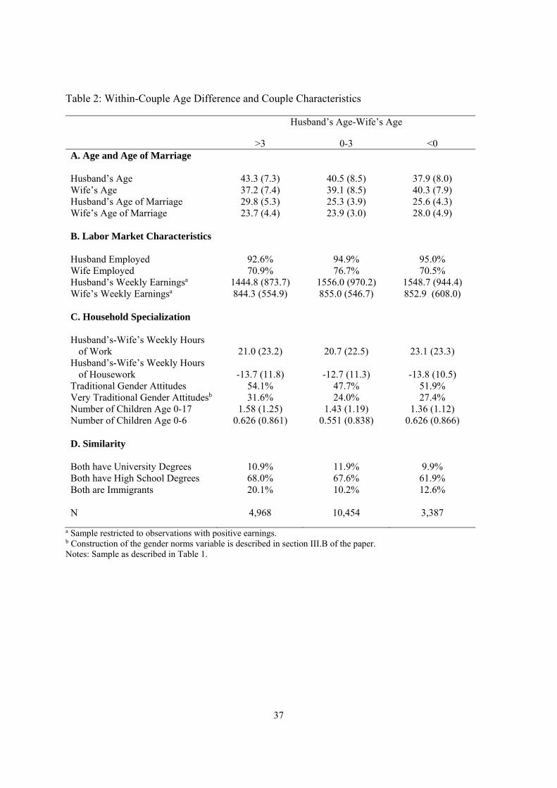
Before estimating the relationship between marital age gap and marital satisfaction, it is

useful to first consider how individual and couple characteristics differ with respect to the marital

age gap. Table 2 sorts couples into three marital age gap categories. The first column reports

variable means for couples in which the husband is more than 3 years older than the wife. The

second column contains couples in which the husband is 0 to 3 years older than the wife. The

third column contains couples in which the wife is older than the husband.

Panel A of Table 2 reports mean age and age of marriage by age gap category. As one

might expect, men who marry younger wives and women who marry younger husbands typically

  13

have older than average ages of marriage. Because they marry at older ages, they are older than

average when they appear in our sample of married couples.

Panel B of Table 2 reports mean employment rates and average weekly earnings (for

positive earners) by age gap category. Men with younger wives have slightly lower employment

rates and lower average weekly earnings than men with similarly-aged or older wives. This is

consistent with analysis by Mansour and McKinnish (2014), who also find that men with

younger wives typically have worse labor market outcomes. Among married women, those

married to similarly-aged husbands have the highest employment rate and highest average

weekly earnings.

Panel C of Table 2 reports descriptive characteristics that are related to the couple’s

degree of household specialization. The first two rows of Panel C indicate that the similarly-aged

couples in column 2 are more similar in work hours and housework hours than the differently-

aged couples in columns 1 and 3. Rows 3 and 4 report measures of the wife’s attitudes towards

traditional gender roles. An indicator variable for traditional gender attitudes equals one if the

wife reports that she agrees with at least 2 of the following 3 statements: “Mothers who don’t

really need the money shouldn’t work,” “It is better for everyone involved if the man earns the

money and the woman takes care of the home and children,” and “A preschool child is likely to

suffer if his/her mother works full time.” An indicator for very traditional gender attitudes

equals one if she agrees with all three statements.11 The results in the table indicate that the wives

with larger marital age gaps are more likely to prefer traditional gender roles.12

                                                            11 More specifically, these gender attitude questions are asked only in 2001, 2005, 2008 and 2011. Couples are labeled as (very) traditional in all survey years if the wife reports agreement with (3) 2 of the statements in any survey year. These three statements were chosen from a larger set of questions about gender roles because they were the three questions that generated the largest variance in responses (on a seven point scale). 12 It has been argued that the level of age homogamy is an important indicator of the egalitarian nature of relationships, as large age differences between spouses have been associated with more patriarchal family systems and less romantic love (Van Poppel et al., 2001; Van de Putte et al., 2009).

  14

The remaining rows of Panel C report mean number of children. Women with younger

husbands have the fewest children, probably because they marry at older ages. Both groups of

differently-aged couples, however, are more likely to have young children than similarly-aged

couples.

Finally Panel D considers whether similarly-aged couples are also similar on other

dimensions. Similarly-aged couples are more likely to have both spouses complete university

degrees, which is consistent with university facilitating age-homogenous marital search.

Similarly-aged couples are not more likely to have both spouses complete high school. Finally,

couples in which the husband is older than the wife are more likely to both be immigrants than

other age gap categories. It could be that immigrant couples are more likely to prefer traditional

older husband and younger wife pairings. It could also be that smaller search pools cause

immigrants to widen their search with respect to the marital age gap.

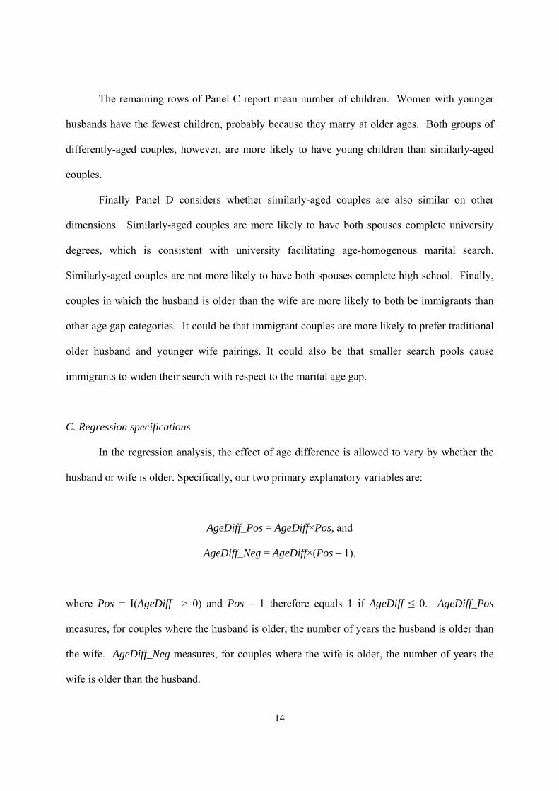
C. Regression specifications

In the regression analysis, the effect of age difference is allowed to vary by whether the

husband or wife is older. Specifically, our two primary explanatory variables are:

AgeDiff_Pos = AgeDiff×Pos, and

AgeDiff_Neg = AgeDiff×(Pos – 1),

where Pos = I(AgeDiff > 0) and Pos – 1 therefore equals 1 if AgeDiff ≤ 0. AgeDiff_Pos

measures, for couples where the husband is older, the number of years the husband is older than

the wife. AgeDiff_Neg measures, for couples where the wife is older, the number of years the

wife is older than the husband.

  15

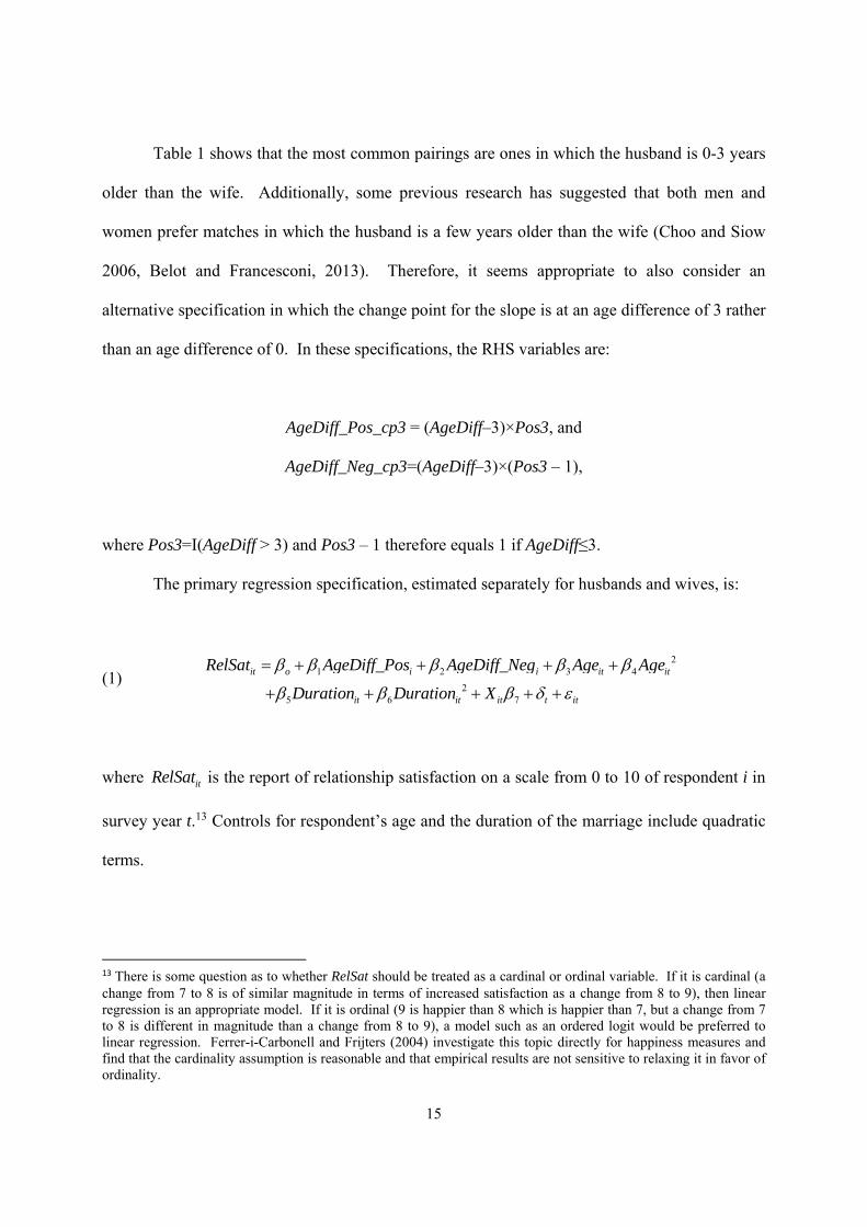
Table 1 shows that the most common pairings are ones in which the husband is 0-3 years

older than the wife. Additionally, some previous research has suggested that both men and

women prefer matches in which the husband is a few years older than the wife (Choo and Siow

2006, Belot and Francesconi, 2013). Therefore, it seems appropriate to also consider an

alternative specification in which the change point for the slope is at an age difference of 3 rather

than an age difference of 0. In these specifications, the RHS variables are:

AgeDiff_Pos_cp3 = (AgeDiff–3)×Pos3, and

AgeDiff_Neg_cp3=(AgeDiff–3)×(Pos3 – 1),

where Pos3=I(AgeDiff > 3) and Pos3 – 1 therefore equals 1 if AgeDiff≤3.

The primary regression specification, estimated separately for husbands and wives, is:

(1) 2

1 2 3 4

25 6 7

it o i i it it

it it it t it

RelSat AgeDiff_Pos AgeDiff_Neg Age Age

Duration Duration X

where itRelSat is the report of relationship satisfaction on a scale from 0 to 10 of respondent i in

survey year t.13 Controls for respondent’s age and the duration of the marriage include quadratic

terms.

                                                            13 There is some question as to whether RelSat should be treated as a cardinal or ordinal variable. If it is cardinal (a change from 7 to 8 is of similar magnitude in terms of increased satisfaction as a change from 8 to 9), then linear regression is an appropriate model. If it is ordinal (9 is happier than 8 which is happier than 7, but a change from 7 to 8 is different in magnitude than a change from 8 to 9), a model such as an ordered logit would be preferred to linear regression. Ferrer-i-Carbonell and Frijters (2004) investigate this topic directly for happiness measures and find that the cardinality assumption is reasonable and that empirical results are not sensitive to relaxing it in favor of ordinality.

  16

itX is a vector of controls that includes the following individual characteristics of both the

husband and wife: education (indicators for high school graduate, post-secondary certification,

bachelor’s degree and graduate degree), employment status indicator, earnings, indicator for

indigenous background, indicator for immigrant status, indicator for chronic health/disability. Xit

also includes the following couple characteristics from Panels C and D of Table 2: difference in

weekly work hours, difference in weekly housework hours, traditional and very traditional

gender attitudes indicators, number of children ages 0-17, number of children ages 0-6, both

spouses have a university degree indicator, both spouses graduated high school indicator, and

both spouses are immigrants indicator. In addition to differences in work hours and housework

hours, husband’s work hours and husband’s housework hours are also included. Finally, itX

includes household-level controls for income, homeownership indicator, house value, indicators

for residence in a city and inner-region of city, local area unemployment and state fixed-effects.

Survey year fixed-effects are also included in the model. Because the sample contains

repeated observations on the same individual, the standard errors are clustered at the individual

level. For some specifications, the age difference variables in equation (1) are replaced by the

variables described above allowing the slope to change at an age difference of 3, rather than an

age difference of 0.

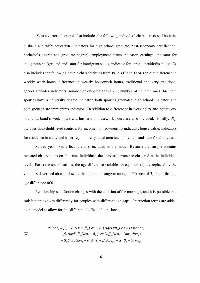
Relationship satisfaction changes with the duration of the marriage, and it is possible that

satisfaction evolves differently for couples with different age gaps. Interaction terms are added

to the model to allow for this differential effect of duration:

(2) 1 2

3 4

25 6 7 8

( )

( )it o i i it

i i it

it it it it t it

RelSat AgeDiff_Pos AgeDiff_Pos Duration

AgeDiff_Neg AgeDiff_Neg Duration

Duration Age Age X

  17

Equations (1) and (2) are pooled cross-section regressions. In these regressions, the

effects of duration and the interaction effects of duration with the age gap variables are estimated

in part by comparing couples who have been married fewer years to couples who have been

married more years. One advantage of the HILDA data is that we observe annual reports of

relationship satisfaction for the same couple over an extended time period, allowing us to include

an individual fixed-effect in order to focus on within-marriage changes in relationship

satisfaction over time:

(3) 1 2

23 4

( ) ( )it o i it i it

it it t i it

RelSat AgeDiff_Pos Duration AgeDiff_Neg Duration

Age X

In the fixed-effects specification, the main effects of the age difference variables are

dropped from the model, as they are perfectly collinear with the individual fixed-effect.

Additionally, when individual fixed-effects are included in the model, the linear terms for age

and marital duration become perfectly collinear with the survey year fixed-effects. This is

because age and duration both change for all respondents by the same amount (1 year) between

survey years. Therefore, it is not possible to estimate the main effect of marital duration on

marital satisfaction in a model that controls for individual fixed-effects. This specification,

however, still allows us to test whether marital satisfaction changes over time differently for

couples with different age gaps.

  18

IV. Results

A. Pooled cross-sectional results

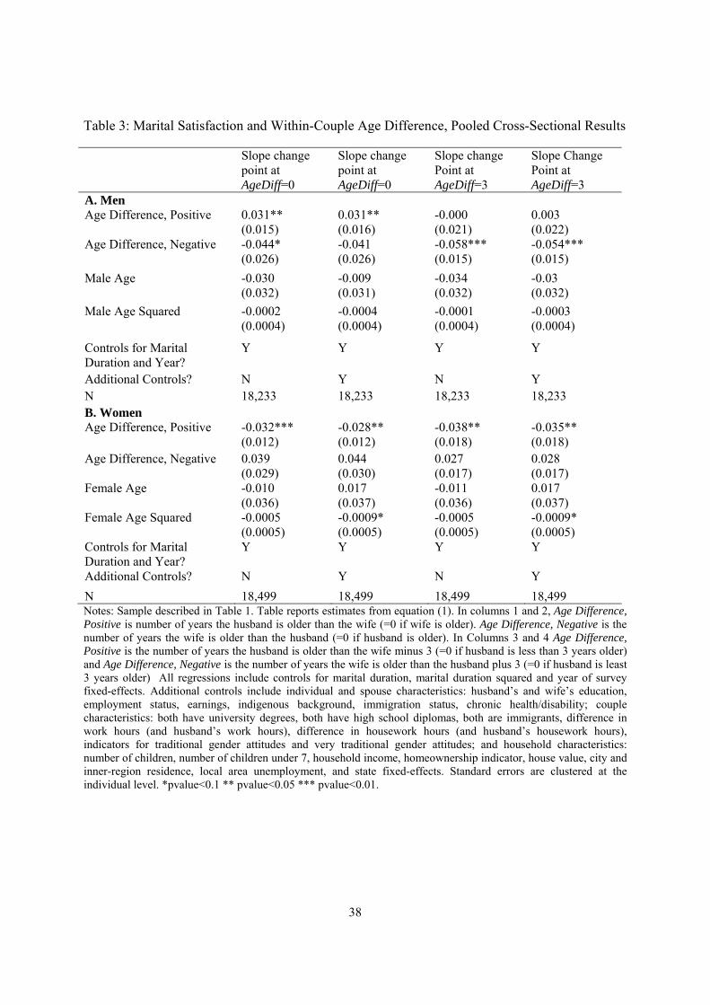
Table 3 reports the results from estimating equation (1) separately for married men and

women.14 Panel A reports the results for men, columns 1 and 2 allowing the slope to differ based

on whether the husband is older or younger than his wife (change point at AgeDiff=0) and

columns 3 and 4 allowing the slope to differ based on whether the husband is more or less than 3

years older than his wife (change point at AgeDiff=3).

The results for men in the first column are obtained only using controls for husband’s age

and age-squared, marital duration and duration squared, and survey year. The estimates indicate

that for husbands with younger wives, every additional year they are older than their wife

increases marital satisfaction on average by 0.031 points. For husbands with older wives, every

additional year their wife is older than they are decreases marital satisfaction on average by

0.044 points. Both effects are statistically significant.

The second column repeats the column one specification, but controlling for the long list

of individual, couple and household controls described above in Section III. Interestingly, the

coefficient estimates are only very modestly changed by the addition of these controls, though

the coefficient on the negative age difference variable does become statistically insignificant.

The third and fourth column results, with the change point at AgeDiff=3, present a

slightly different picture. For men who are more than 3 years older than their wives, an

additional year of age gap with their wife does not change their reported relationship satisfaction.

For men who are no more than 3 years older than their wife, every additional year their wife is

older relative to their own age reduces their relationship satisfaction by 0.054 points.

                                                            14 Sample sizes differ slightly for men and women because there is a relatively modest number of observations for which we only have either the wife’s or the husband’s marital satisfaction report.

  19

The results for women are reported in panel B. For women with older husbands, every

additional year their husband is older than them decreases their satisfaction by 0.032. For

women with younger husbands, every additional year their husband is younger than them

increases marital satisfaction by 0.039, but the coefficient is not statistically significant. The

results for women in columns 1 and 2 are surprisingly symmetric with the results for men, with

quite similar coefficient magnitudes, just of opposite sign.

Columns 3 and 4 report the results for women when the slope is allowed to change at

AgeDiff=3 instead of AgeDiff=0. Unlike the results for men, the results for women are more

modestly affected by this change in specification.

Overall, the results in Table 3 indicate that both men and women experience greater

marital satisfaction when married to younger partners. These results are more consistent with the

Coles and Francesconi (2011) assumption that both men and women receive higher utility from

younger spouses, than with the Bergstrom and Bagnoli (1993) prediction that both men and

women receive the greatest marital gains in older husband-younger wife pairings or with the

Choo and Siow (2006) estimates, which suggest that net marital gains are greatest for couples in

which the husband is just a few years older than the wife. The symmetry of estimates for men

and women is inconsistent with Diaz-Gimenez and Giolito (2013), who predict that men receive

the greater disutility from marrying older partners, given the more rapidly declining fecundity of

women.

It would be premature, however, to argue that our results confirm the Coles and

Francesconi (2011) model, as that model predicts that individuals will trade off one attribute

(partner youth and “fitness”) with another (partner income). If most individuals entering into

relationships with older spouses were doing so because they were being compensated for the

disutility of marrying an older partner by the higher income of the older spouse, we would expect

  20

our marital satisfaction results to be sensitive to controls for partner’s education, work hours and

earnings. The fact that the results are very robust to controls for partner characteristics suggests

that this trade-off is not a primary explanation for differently-aged pairings.15

Additionally, the fact that men and women both report greater marital satisfaction when

married to younger partners seems at odds with the dating literature results that men and women

are both more likely to prefer similarly-aged dates (Belot and Francesconi, 2013; Hitsch,

Hortacsu and Ariely, 2010). Our marital satisfaction results suggest that men and women may

choose to contact similarly-aged partners in online and speed-dating settings for strategic

reasons, taking into account the age gap preferences of the potential partners, rather than because

they themselves prefer similarly-aged spouses. Support for this notion can be found in Antfolk et

al. (2015) who find using data on preferred partner’s age and actual partner’s age that although

men revealed a tendency to be sexually interested in women in their mid-twenties, they tended to

partner up with similar-aged females in real life. The authors suggest that men’s heterosexual

activity is likely to be constrained by female choice.

B. Interaction between age difference and marital duration

Tables 4 and 5 report the results from estimating equations (2) and (3). These

specifications include interaction effects of the age difference variables with marital duration.

Table 4 reports the results for husband’s marital satisfaction and Table 5 reports the results for

wife’s marital satisfaction. In both tables, Panel A uses the same age difference variables used in

columns 1 and 2 of Table 2, which allow the slope to change at AgeDiff=0, while Panel B reports

                                                            15 One possible explanation for the insensitivity of the age difference estimates in Table 3 to the addition of a large number of individual, couple and household controls is that different controls act to move the age difference coefficients in different directions, ultimately cancelling each other out. We find, however, that is not the case. When we add the controls in small sets, we find the same degree of insensitivity of the age difference coefficient estimates.

  21

the results using the age difference variables used in columns 3 and 4 of Table 3, which allow the

slope to change at AgeDiff=3.

In Panel A of Table 4, the pooled cross-section results reported in column 1 show that the

main effect of the positive age difference variable is positive and statistically significant. This

indicates that at the beginning of the marriage, men derive greater satisfaction from being

married to younger wives. The coefficient on marital duration is positive, implying that marital

satisfaction increases over time. This estimate must be interpreted with caution, however, as this

likely reflects the fact that couples surviving to greater marital durations were happier to begin

with. The coefficients on the interactions of the age difference variables with duration are

negative, though statistically insignificant. These interaction terms indicate that relative to the

positive main effect of marital duration, marital satisfaction increases at a slower rate for

husbands with differently-aged spouses compared to husbands with similarly-aged spouses.

When individual fixed-effects are added to the model in column 2, the main effects of the

age difference variables and the main effect of marital duration can no longer be estimated. The

interaction of positive age difference with duration becomes more negative and statistically

significant. While men married to younger wives start out more satisfied, their marital

satisfaction declines relative to men married to similarly-aged wives over the duration of the

marriage. The magnitude of the coefficient (-0.005), when compared to the coefficient on the

main effect of positive age difference in column 1 (0.040), suggests that the greater marital

satisfaction enjoyed by men with younger wives dissipates by the 8th year of marriage. Marital

satisfaction for men married to older wives also declines relative to men with similarly-aged

wives, but the coefficient is not statistically significant.

Table 2 indicated that differently-aged couples differ in their degree of household

specialization compared to similarly-aged couples. This suggests that differently-aged couples

  22

and similarly-aged couples may typically generate marital gains from different sources (e.g.

household specialization versus joint investment and consumption). It is possible that different

sources of marital gains will differ in how well the gains persist over the duration of the

marriage. Column 3 of Table 4 therefore adds additional interaction terms that allow for the

possibility that more-specialized couples experience different trends in marital satisfaction than

less-specialized couples. Specifically, marital duration is interacted with 3 time-constant

variables: 1) A specialized couple indicator that equals 1 if the couple is in the top quartile of

average difference in work hours or average difference in housework hours, where work hours

and housework hours have been averaged across all survey years; 2) The very traditional gender

attitudes indicator reported in Table 2; and 3) The maximum total number of children ever

reported by the couple in the survey across all survey years.

Most importantly, the results in column 3 indicate that the age difference interactions are

insensitive to these additional controls.16 Of the three additional interaction variables, only the

interaction of marital duration with total number of children is statistically significant. The

coefficient estimate indicates that couples with more children experience increases in marital

satisfaction over the duration of the marriage relative to couples with fewer children. This result,

however, must be interpreted with caution, as couples that are happier and last longer will be

more likely to have more children. We reconsider this result in the next section.

Panel B of Table 4 repeats the same analysis for men, but using the age-difference

variables from columns 3 and 4 of Table 3, which allow the slope to change at an age difference

of 3. In Table 3, we reported that the coefficient on the positive age difference variable for men

becomes small and insignificant when the slope change point is shifted from 0 years to 3 years.

                                                            16 We also find that the results are similar if we experiment with stricter definitions of specialization (for example, being in the top quartile for both the mean difference in work hours and mean difference in housework hours), use the traditional gender roles indicator instead of very traditional indicator, or add an interaction of marital duration with an indicator variable that both spouses are immigrants.

  23

In Table 4, we see that this null effect masked considerable heterogeneity by marital duration.

These results indicate that there is a higher level of marital satisfaction for men with much

younger wives at the beginning of the marriage, this higher level of satisfaction dissipates rather

rapidly and is erased after 6 to 10 years of marriage. Therefore, the null result in Table 2

reflected the fact that we were averaging the marital satisfaction of men with younger wives

across marriages of different marital duration. Overall, the results in Panel B of Table 4 are very

similar to those in Panel A.

Table 5 uses the same specifications as Table 4, but reports the results for women. The

results in Panel A indicate that, compared to women married to similarly-aged husbands, marital

satisfaction declines over time both for women married to older husbands and women married to

younger husbands. If we compare the coefficients on the interaction of marital duration with the

negative age difference variable in columns 2 and 3 (-0.009) to the main effect of negative age

difference reported in column 2 (0.049), this suggests that the initial higher-level of marital

satisfaction experienced by women married to younger husbands is erased by the 6th year of

marriage.

The results in Panel B of Table 5 are consistent with those in Panel A, though the

coefficient on the positive age difference interaction becomes larger in magnitude, while the

coefficient on the negative age difference variable becomes smaller and insignificant.

Additionally, the coefficient estimates on the additional interactions of marital duration with the

household specialization measures are very similar to those obtained for husband’s satisfaction in

Table 4.

Overall, the results in Tables 4 and 5 suggest that couples with larger marital age gaps

experience declines in marital satisfaction over the duration of the marriage relative to couples

with smaller age gaps. These declines erase the initial higher levels of satisfaction experienced

  24

by husbands married to younger wives and wives married to younger husbands within 6-10 years

of marriage.

C. Sample selection

While the fixed-effects results in columns 2 and 3 of Tables 4 and 5 are estimated using

within-marriage changes over time in marital satisfaction, some couples exit the sample due to

divorce. This raises the concern that even the fixed-effects estimates are biased by sample-

selection, because only surviving couples are observed at longer marital durations. To check for

the robustness of our results to selection out of marriage, in column 4 of Tables 4 and 5, the

sample is restricted to only include couples who never separate during the HILDA survey years.

We further restrict the sample to only include couples who are observed for at least 8 years.

The coefficients on the age-difference interactions for men (Table 4, column 4) and

women (Table 5, column 4) using this restricted sample are very similar to the results using the

unrestricted sample (column 3 of Tables 4 and 5 respectively), suggesting that these results are

largely unaffected by sample selection through divorce. Interestingly, this change in sample has

a substantial effect on the coefficient estimate for the interaction of marital duration with number

of children. The coefficient changes from positive and significant to negative and significant.

This sign reversal highlights the concern raised above, that the positive coefficient in the

unrestricted sample likely reflects the fact that happier, longer last couples have more children.

The change in the coefficient estimate when the sample is limited to long-term couples shows

that this sample restriction can be effective at revealing which results are driven by sample

selection into longer marital durations.

The self-selection process not only selects happier marriages into the sample over time,

there is likely also to be selection into marriage with low or high age differences. Given the

  25

possible endogeneity of the marital age gap, it would be useful to pursue an instrumental variable

strategy. In our application, two instruments would be required, one for AgeDiff_Pos and another

for AgeDiff_Neg. Following Meng and Gregory (2005) who utilized the probability of marrying

within one’s ethnic-religion-age group and sex ratios as instruments for ethnic intermarriage, we

pursued a strategy of creating instruments using male and female sex ratios based on location

(state) and age in the year of marriage and alternatively in the year the individual turned 20.

These sex ratios reflect the availability of potential partners at the time of marriage and arguably

affect the marital age gap but not marital satisfaction directly. For multiple endogenous

variables, inspection of the standard first-stage F-statistics is no longer sufficient and the

conditional F-statistic is required (Sanderson and Windmeijer, 2016). Unfortunately, the

conditional F-statistic suggests that the instruments are weak for the possible endogenous

regressors. Lacking a credible instrument, we therefore were unable to pursue this empirical

strategy in this paper.

D. Differences in marital satisfaction between husband and wife

Because the HILDA survey elicits relationship satisfaction data from both members of

the couple, it is possible to use the difference in husband’s and wife’s satisfaction as the

dependent variable. This requires a change in the model specification. Previously, when the

dependent variable was husband’s satisfaction, husband’s age and age-difference with wife were

both included as independent variables. Likewise, when the dependent variable was wife’s

satisfaction, the wife’s age and age-difference with husband were both included as independent

variables. If husband’s and wife’s satisfaction will appear jointly on the left-hand side of the

regression, the most obvious approach would therefore be to include husband’s age, wife’s age

and age-difference between husband and wife as independent variables, but it is not possible to

  26

separately identify all three of these variables in the same regression. Therefore, the regressions

using difference in husband’s and wife’s satisfaction as the dependent variable will use

husband’s age and wife’s age as independent variables.

Table 6 builds up to this specification by first, in columns 1 and 2, separately regressing

husband’s and wife’s satisfaction on both husband’s and wife’s ages. The results in column 1

indicate that wife’s age is a much stronger predictor of husband’s satisfaction than husband’s

age. Controlling for husband’s age, husband’s satisfaction decreases as wife’s age increases.

The results for wives in column 2 follow a very similar pattern. Husband’s age is a stronger

predictor of wife’s satisfaction than wife’s age, and controlling for wife’s age, wife’s satisfaction

decreases as husband’s age increases. Thus, for both genders, controlling for own age, marital

satisfaction is decreasing in partner’s age.

In column 3 of Table 6, the dependent variable is husband’s satisfaction minus wife’s

satisfaction. It is easy to see, by looking across the first two columns, that the negative effect of

husband’s age on wife’s satisfaction dominates its effect on husband’s satisfaction. Therefore,

controlling for wife’s age, an older husband is associated with a larger gap between husband’s

and wife’s satisfaction. Similarly, the negative effect of wife’s age on husband’s satisfaction

dominates its effect on wife’s satisfaction. Therefore, controlling for husband’s age, an older

wife is associated with a smaller gap between husband’s and wife’s satisfaction by decreasing

husband’s satisfaction relative to wife’s satisfaction.

These results in Table 6 are consistent with our findings in Table 3 that men are more

satisfied and women are less satisfied as the age gap between husband and wife increases. To

provide some context for the estimates in column 3, the average difference in marital satisfaction

between husband and wife for same-aged couples in our sample is 0.065. This is consistent with

the descriptive analysis in Table 1 and Figures 1 and 2, which showed that husbands on average

  27

tend to report greater marital satisfaction than wives. This combined with the positive

coefficient on husband’s age in column 3 indicates that couples in which the husband is older

than the wife will typically experience even larger gaps in marital satisfaction. The negative

coefficient on wife’s age indicates that couples in which the wife is older than the husband will

typically experience smaller gaps in satisfaction between the husband and wife, with couples in

which the wife is 4 years older predicted to roughly “break even” with a marital satisfaction gap

close to zero. It should be noted that couples in which the wife is 4 or more years older than the

husband are relatively rare, only 3.6% of our sample.

Column 4 includes interaction effects with marital duration, and shows that the main

effect of husband’s age estimated in column 3 becomes more pronounced the longer the couple

has been married. This suggests that the positive marital satisfaction gap between husband and

wife widens more over time for marriages with a more positive marital age gap. This interaction

effect, however, become statistically insignificant once individual fixed-effects are added to the

model.

E. Negative economic shocks and marital satisfaction

Compared to similarly-aged couples, both men and women in differently-aged couples

experience larger declines in marital satisfaction over the duration of the marriage. One potential

mechanism is that when couples experience negative shocks, differently-aged couples experience

a greater loss in marital satisfaction than similarly-aged couples. Put another way, similarly-

aged couples are more resilient to negative shocks than differently-aged couples. This could be

the case, for example, if differently-aged couples have less similar preferences, making it harder

for them to agree on how to adjust consumption in response to a negative economic shock.

  28

We test for evidence of this mechanism in Table 7. HILDA respondents are asked if they

have experienced a “major worsening in financial situation (e.g. went bankrupt)” in the past year.

26.2% of couples in our sample report at least one such negative economic shock, 11.5% report

more at least two negative economic shocks, but only 2.5% report more than two such shocks.

In Panel A of Table 7, we regress marital satisfaction on an indicator for reporting a worsening

of finances, and also interact this indicator with the age-difference variables.17 The first two

columns of Table 7 report the results for men and columns 3 and 4 report the results for women.

Columns 1 and 3 report results without individual fixed-effects and columns 2 and 4 report

results controlling for individual fixed-effects.

The results for both men and women in Panel A indicate that differently-aged couples,

both those with an older wife and those with an older husband, experience larger declines in

marital satisfaction in response to a negative economic shock than similarly-aged couples. For

men, both of the interaction terms are negative and statistically significant. For women, while

both interaction terms are negative, only the interaction with the positive age difference variable

is statistically significant. The interaction with the negative age difference variable, while

insignificant, is more negative in magnitude than the interaction with positive age difference.

Panel B performs a similar analysis using reports of whether the couple experienced a

health shock (“serious personal injury or illness”) in the past year. 43.8% of couples in our

sample report at least one health shock, but only 3.6 percent report three or more. The pooled

estimates reported in columns 1 and 3, while statistically insignificant; also indicate that

differently-aged couples experience larger declines in marital satisfaction than differently-aged

                                                            17 Controls for husband’s and wife’s age and age-squared, marital duration and duration-squared, and year fixed-effects are included in the regressions, as well as the additional controls used in Tables 2-4, except economic controls (employment, earnings, household income and house value). It would be inappropriate to include these controls given that they could control for much of the effect of a negative economic shock.

  29

couples. The estimates in columns 2 and 4, however, once individual fixed-effects are included

in the model, are much more mixed.

V. Conclusions

Our results indicate that marital satisfaction varies with the marital age gap.

Specifically, we find that in the first 6-10 years of marriage, both men and women are most

satisfied with younger partners and least satisfied with older partners. Our analysis of the

interaction between marital satisfaction and marital age gap suggests that marital satisfaction

declines more rapidly over time for both men and women in differently-aged couples compared

to similarly-aged couples, so that after 6-10 years, the initial higher levels of satisfaction

experienced by men married to younger wives and women married to younger husbands are

erased. Finally, our analysis suggests a potential mechanism for the relative declines in the

satisfaction of differently-aged couples, which is that differently-aged couples experience larger

declines in marital satisfaction in response to a negative economic shock compared to similarly-

aged couples.

Our finding that, in the cross-section, both men and women are the most satisfied with

younger partners and least satisfied with older partners, contradicts much of the existing

literature on marital sorting and marital age gaps. For example, our results are at odds with the

theoretical model of Bergstrom and Bagnoli (1993) which predicts that older husband-younger

wife pairings experience the greatest marital gains. Our results are also inconsistent with the

Choo and Siow (2006) estimates which indicate that net marital gains are maximized by pairings

in which the husband is a few years older than the wife. While our result are consistent with the

Coles and Francesconi (2011) assumption that both men and women prefer younger, “fitter”

spouses, the insensitivity of our estimates to controls for partner’s earnings is inconsistent with

  30

their prediction that men and women who marry older spouses are being compensated for their

disutility by the higher earnings of the older spouse. Finally, the symmetry of the effect of

marital age gap on marital satisfaction between men and women is inconsistent with Diaz-

Gimenez and Giolito (2013), who predict a greater disutility from older partners for men, due to

women’s more rapidly declining fecundity.

Our results also call into question the preference estimates generated using data from

online data and speed-dating events. The fact that both men and women tend to seek dates with

similarly-aged partners had previously been interpreted as evidence that both men and women

prefer similarly-aged partners (Berlot and Francesconi, 2013; Hitsch, Hortacsu and Ariely,

2010). But this interpretation is only valid if men and women do not strategically take into

account their probability of success when choosing who to contact. The fact that men, at least

initially, experience high levels of marital satisfaction when married to younger wives, but

women experience lower levels of marital satisfaction when married to older husbands, suggests

that men may actually prefer to seek dates with younger partners, but avoid doing so because

they know that they would only be successful with low-quality younger partners. The same

reasoning may also explain why women avoid seeking dates with younger men.18

While several theoretical papers in economics focus on the rationale for the formation of

differently-aged couples, there are no theoretical predictions regarding how the marital

satisfaction of differently-aged couples will evolve over time. While our analysis indicates that

differently-aged couples are more vulnerable to economic shocks, there might be other

                                                            18 An alternative explanation is that individuals are sufficiently forward looking when selecting spouses to recognize that their initial higher levels of marital satisfaction with a younger spouse will dissipate, as we find. They might then prefer similarly-aged spouses, to the extent that they generate the greater net present discounted value of lifetime marital satisfaction. Given it takes about 10 years for the benefit of marrying a younger spouse to dissipate, this would likely, however, require that an individual have both a low discount rate and a low subjective probability of divorce. Additionally, to the extent that the declines in satisfaction we observe are due in part to the larger negative effects of unanticipated shocks, individuals may not be able to anticipate these declines adequately to prefer a similarly-aged spouse.

  31

mechanisms through which marital age gap affects the evolution of marital satisfaction over

time. For example, the fact that the husband and wife are in different points of their life-cycle

may have different effects on marital satisfaction at different points in the marriage, such as

when one partner wants to have children or when one partner wants to retire. Future research

might want to explore in more depth why marital satisfaction declines more quickly over time

for both men and women in differently-aged couples as compared to similarly-aged couples.

This future research should also more fully address the empirical implications of selection into

marriage of couples with different age gaps, as well as the selection of married couples into

longer marital durations.

  32

References Antfolk, J., B. Salo, K. Alanko, E. Bergen, J. Corander, N. Sandnabba and P. Santtila. (2015). Women's and Men's Sexual Preferences and Activities with Respect to the Partner's Age: Evidence for Female Choice. Evolution and Human Behavior, 36: 73–79. Amato, P., A. Booth, D. Johnson and S. Rogers. (2007). Alone Together: How Marriage in America is Changing. Cambridge, MA: Harvard University Press. Becker, G, E. Landes and R. Michael. (1977). An Economic Analysis of Marital Instability. Journal of Political Economy, 85: 1141-87. Belot, M. and M. Francesconi. (2013). Dating Preferences and Meeting Opportunities in Mate Choice Decisions. Journal of Human Resources, vol. 48: 474–508. Bergstrom, T. and M. Bagnoli. (1993). Courtship as a Waiting Game, Journal of Political Economy, 101: 185–201. Cherlin. A. (1977). The Effect of Children on Marital Dissolution. Demography 14: 265–272. Choo, E., and A. Siow. (2006). Who Marries Whom and Why, Journal of Political Economy 114: 175-201. Coles, M. and M. Francesconi. (2011). On the Emergence of Toyboys: the Timing of Marriage with Aging and Uncertain Careers. International Economic Review, 52: 825–853. Diaz-Gimenez, J. and E. Giolito. (2013). Accounting for the Timing of First Marriage. International Economic Review, 54: 135–158. Drefahl, S. (2010). How does the Age Gap Between Partners Affect their Survival? Demography, 47: 313–326. Ferrer-i-Carbonell, A. and P. Frijters. (2004). How Important is Methodology for the Estimates of the Determinates of Happiness? The Economic Journal, 114:641-59. Fisman, R., S. Iyengar, E. Kamenica and I. Simonson. (2006). Gender Differences in Mate Selection: Evidence from a Speed Dating Experiment. The Quarterly Journal of Economics, 121: 673-697. Glenn, N. (1998). The Course of Marital Success and Failure in Five American 10-year Marriage Cohorts. Journal of Marriage and Family, 60: 569–576. Glick, P. and S-L Lin. (1986). Recent Changes in Divorce and Remarriage. Journal of Marriage and Family, 48: 737–747. Groot, W. and H. Van Den Brink. (2002). Age and Education Differences in Marriages and their Effects on Life Satisfaction. Journal of Happiness Studies, 3: 153-165.

  33

Hitsch, G., A. Hortascsu and D. Ariely. (2010). Matching and Sorting in Online Dating. American Economic Review, 100: 130–163. Lillard, L., M. Brien and L. Waite. (1995). Premarital Cohabitation and Subsequent Marital Dissolution: A Matter of Self Selection. Demography, 32: 437–457. Mansour, H. and T. McKinnish. (2014). Who Marries Differently Aged Spouses? Ability, Education, Occupation, Earnings, and Appearance. Review of Economics and Statistics, 96: 577–580. Meng, X. and Gregory, R.G. (2005). Intermarriage and Economic Assimilation of Immigrants, Journal of Labor Economics, 23: 135–176. Presser, H. (1975). Age Differences between Spouses, American Behavioral Scientist, 19: 190–205. Rogler, L. and M. Procidano. (1989). Marital Heterogamy and Marital Quality in Puerto Rican Families, Journal of Marriage and Family, 51: 363–372. Sanderson, E. and F. Windmeijer (2016). A Weak Instrument F-test in Linear IV Models with Multiple Endogenous Variables. Journal of Econometrics, 190: 212–221. Siow, A. (1998). Differential Fecundity, Markets, and Gender Roles. Journal of Political Economy, 106: 334–354. Van Poppel, F., A. Liefbroer, J. Vermunt and W. Smeenk. (2001). Love, Necessity and Opportunity: Changing Patterns of Marital Age Homogamy in the Netherlands, 1850–1993. Population Studies, 55: 1–13. Van De Putte, B., F. Van Poppel, S. Vanassche et al. (2009). The Rise of Age Homogamy in 19th Century Western Europe. Journal of Marriage and Family, 47: 1234–1253. Van Laningham, J., D. Johnson and P. Amato. (2001). Marital Happiness, Marital Duration, and the U-shaped Curve: Evidence from a Five-Wave Panel Study. Social Forces, 78: 1313–1341. Vera, H., D. Berardo and F. Berardo. (1985). Age Heterogamy in Marriage. Journal of Marriage and Family, 47: 553–566. Weiss, Y. and R. Willis. (1997). Match quality, New Information, and Marital Dissolution. Journal of Labor Economics, 15:S293-S329. Wood, S. (2006). Low-rank Scale-invariant Tensor Product Smooths for Generalized Additive Mixed Models. Biometrics, 62: 1025–1036. Zhang, H., P. Ho and P. Yip. (2012). Does Similarity Breed Marital and Sexual Satisfaction? Journal of Sex Research, 49: 583–593.

  34

Figure 1: Husband’s marital satisfaction by marital duration and marital age gap, conditional on husband’s age and age-squared

  35

Figure 2: Wife’s marital satisfaction by marital duration and marital age gap, conditional on wife’s age and age-squared

  36

Table 1: Within-Couple Age Difference and Marital Satisfaction, Descriptive Statistics

Husband’s Age –Wife’s Age

N % Mean Husband’s Satisfaction

Mean Wife’s Satisfaction

+7 or more

299

8.9

8.46

8.28

+4 to 6

608

18.0

8.48

8.28

+1 to 3

1,375

40.8

8.54

8.35

0

499

14.8

8.43

8.32

-1 to -3

469

13.9

8.39

8.34

-4 to -6

89

2.6

8.38

8.36

-7 or more

35

1.0

7.81

8.25

Notes: Sample of couples observed in a first marriage in HILDA 2001-2013 data where husband and wife are both in their first marriage and ages 20-55. There are 3,374 couples in our sample and 18,987 couple-years. Each couple receives equal weight in the means reported in columns 3 and 4, regardless of the number of years of data.

  37

Table 2: Within-Couple Age Difference and Couple Characteristics

Husband’s Age-Wife’s Age

>3 0-3 <0 A. Age and Age of Marriage Husband’s Age

43.3 (7.3)

40.5 (8.5)

37.9 (8.0) Wife’s Age 37.2 (7.4) 39.1 (8.5) 40.3 (7.9) Husband’s Age of Marriage 29.8 (5.3) 25.3 (3.9) 25.6 (4.3) Wife’s Age of Marriage 23.7 (4.4) 23.9 (3.0) 28.0 (4.9) B. Labor Market Characteristics Husband Employed

92.6%

94.9%

95.0% Wife Employed 70.9% 76.7% 70.5% Husband’s Weekly Earningsa 1444.8 (873.7) 1556.0 (970.2) 1548.7 (944.4) Wife’s Weekly Earningsa 844.3 (554.9) 855.0 (546.7) 852.9 (608.0) C. Household Specialization Husband’s-Wife’s Weekly Hours

of Work

21.0 (23.2)

20.7 (22.5)

23.1 (23.3) Husband’s-Wife’s Weekly Hours

of Housework

-13.7 (11.8)

-12.7 (11.3)

-13.8 (10.5) Traditional Gender Attitudes 54.1% 47.7% 51.9% Very Traditional Gender Attitudesb 31.6% 24.0% 27.4% Number of Children Age 0-17 1.58 (1.25) 1.43 (1.19) 1.36 (1.12) Number of Children Age 0-6 0.626 (0.861) 0.551 (0.838) 0.626 (0.866) D. Similarity Both have University Degrees

10.9%

11.9%

9.9% Both have High School Degrees 68.0% 67.6% 61.9% Both are Immigrants 20.1% 10.2% 12.6% N 4,968 10,454 3,387

a Sample restricted to observations with positive earnings. b Construction of the gender norms variable is described in section III.B of the paper. Notes: Sample as described in Table 1.

  38

Table 3: Marital Satisfaction and Within-Couple Age Difference, Pooled Cross-Sectional Results

Slope change point at AgeDiff=0

Slope change point at AgeDiff=0

Slope change Point at AgeDiff=3

Slope Change Point at AgeDiff=3

A. Men Age Difference, Positive

0.031** (0.015)

0.031** (0.016)

-0.000 (0.021)

0.003 (0.022)

Age Difference, Negative -0.044* (0.026)

-0.041 (0.026)

-0.058*** (0.015)

-0.054*** (0.015)

Male Age -0.030 (0.032)

-0.009 (0.031)

-0.034 (0.032)

-0.03 (0.032)

Male Age Squared -0.0002 (0.0004)

-0.0004 (0.0004)

-0.0001 (0.0004)

-0.0003 (0.0004)

Controls for Marital Duration and Year?

Y Y Y Y

Additional Controls? N Y N Y N 18,233 18,233 18,233 18,233 B. Women Age Difference, Positive

-0.032*** (0.012)

-0.028** (0.012)

-0.038** (0.018)

-0.035** (0.018)

Age Difference, Negative 0.039 (0.029)

0.044 (0.030)

0.027 (0.017)

0.028 (0.017)

Female Age -0.010 (0.036)

0.017 (0.037)

-0.011 (0.036)

0.017 (0.037)

Female Age Squared -0.0005 (0.0005)

-0.0009* (0.0005)

-0.0005 (0.0005)

-0.0009* (0.0005)

Controls for Marital Duration and Year?

Y Y Y Y

Additional Controls? N Y N Y

N 18,499 18,499 18,499 18,499 Notes: Sample described in Table 1. Table reports estimates from equation (1). In columns 1 and 2, Age Difference, Positive is number of years the husband is older than the wife (=0 if wife is older). Age Difference, Negative is the number of years the wife is older than the husband (=0 if husband is older). In Columns 3 and 4 Age Difference, Positive is the number of years the husband is older than the wife minus 3 (=0 if husband is less than 3 years older) and Age Difference, Negative is the number of years the wife is older than the husband plus 3 (=0 if husband is least 3 years older) All regressions include controls for marital duration, marital duration squared and year of survey fixed-effects. Additional controls include individual and spouse characteristics: husband’s and wife’s education, employment status, earnings, indigenous background, immigration status, chronic health/disability; couple characteristics: both have university degrees, both have high school diplomas, both are immigrants, difference in work hours (and husband’s work hours), difference in housework hours (and husband’s housework hours), indicators for traditional gender attitudes and very traditional gender attitudes; and household characteristics: number of children, number of children under 7, household income, homeownership indicator, house value, city and inner-region residence, local area unemployment, and state fixed-effects. Standard errors are clustered at the individual level. *pvalue<0.1 ** pvalue<0.05 *** pvalue<0.01.

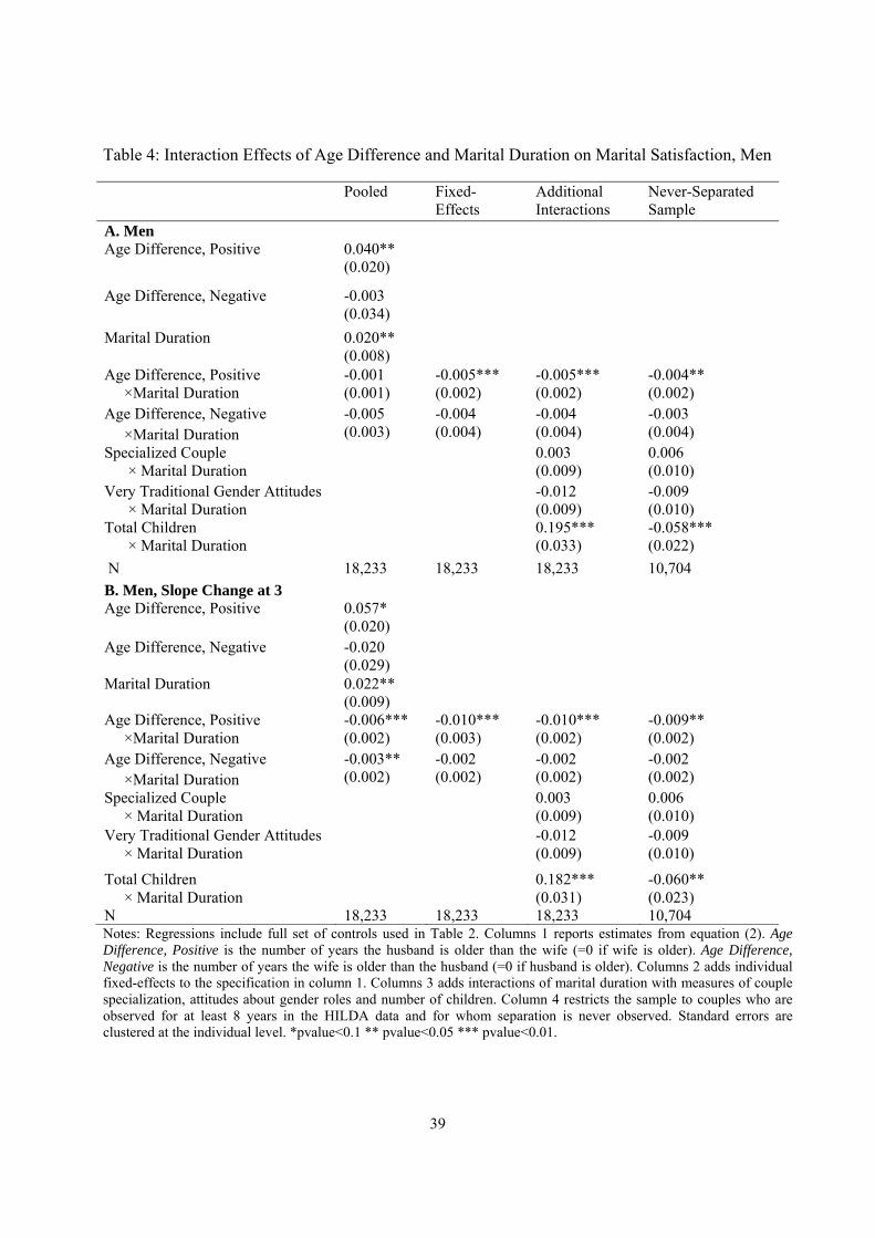
  39

Table 4: Interaction Effects of Age Difference and Marital Duration on Marital Satisfaction, Men

Pooled Fixed-Effects

Additional Interactions

Never-Separated Sample

A. Men Age Difference, Positive

0.040** (0.020)

Age Difference, Negative

-0.003 (0.034)

Marital Duration 0.020** (0.008)

Age Difference, Positive ×Marital Duration

-0.001 (0.001)

-0.005*** (0.002)

-0.005*** (0.002)

-0.004** (0.002)

Age Difference, Negative ×Marital Duration

-0.005 (0.003)

-0.004 (0.004)

-0.004 (0.004)

-0.003 (0.004)

Specialized Couple × Marital Duration

0.003 (0.009)

0.006 (0.010)

Very Traditional Gender Attitudes × Marital Duration

-0.012 (0.009)

-0.009 (0.010)

Total Children × Marital Duration

0.195*** (0.033)

-0.058*** (0.022)

N 18,233 18,233 18,233 10,704

B. Men, Slope Change at 3 Age Difference, Positive

0.057* (0.020)

Age Difference, Negative -0.020 (0.029)

Marital Duration 0.022** (0.009)

Age Difference, Positive ×Marital Duration

-0.006*** (0.002)

-0.010*** (0.003)

-0.010*** (0.002)

-0.009** (0.002)

Age Difference, Negative ×Marital Duration

-0.003** (0.002)

-0.002 (0.002)

-0.002 (0.002)

-0.002 (0.002)

Specialized Couple × Marital Duration

0.003 (0.009)

0.006 (0.010)

Very Traditional Gender Attitudes × Marital Duration

-0.012 (0.009)

-0.009 (0.010)

Total Children × Marital Duration

0.182*** (0.031)

-0.060** (0.023)

N 18,233 18,233 18,233 10,704 Notes: Regressions include full set of controls used in Table 2. Columns 1 reports estimates from equation (2). Age Difference, Positive is the number of years the husband is older than the wife (=0 if wife is older). Age Difference, Negative is the number of years the wife is older than the husband (=0 if husband is older). Columns 2 adds individual fixed-effects to the specification in column 1. Columns 3 adds interactions of marital duration with measures of couple specialization, attitudes about gender roles and number of children. Column 4 restricts the sample to couples who are observed for at least 8 years in the HILDA data and for whom separation is never observed. Standard errors are clustered at the individual level. *pvalue<0.1 ** pvalue<0.05 *** pvalue<0.01.

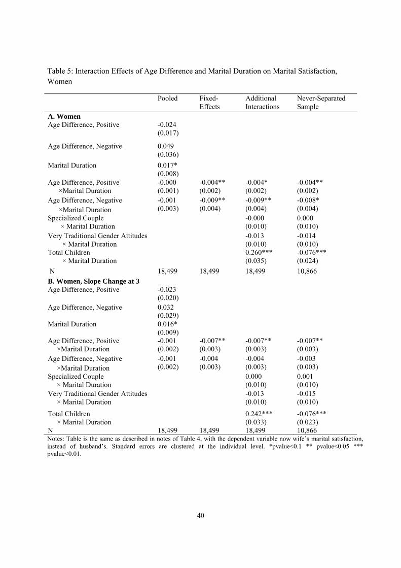
  40

Table 5: Interaction Effects of Age Difference and Marital Duration on Marital Satisfaction, Women

Pooled Fixed-Effects

Additional Interactions

Never-Separated Sample

A. Women Age Difference, Positive

-0.024 (0.017)

Age Difference, Negative

0.049 (0.036)

Marital Duration 0.017* (0.008)

Age Difference, Positive ×Marital Duration

-0.000 (0.001)

-0.004** (0.002)

-0.004* (0.002)

-0.004** (0.002)

Age Difference, Negative ×Marital Duration

-0.001 (0.003)

-0.009** (0.004)

-0.009** (0.004)

-0.008* (0.004)

Specialized Couple × Marital Duration

-0.000 (0.010)

0.000 (0.010)

Very Traditional Gender Attitudes × Marital Duration

-0.013 (0.010)

-0.014 (0.010)

Total Children × Marital Duration

0.260*** (0.035)

-0.076*** (0.024)

N 18,499 18,499 18,499 10,866

B. Women, Slope Change at 3 Age Difference, Positive

-0.023 (0.020)

Age Difference, Negative 0.032 (0.029)

Marital Duration 0.016* (0.009)

Age Difference, Positive ×Marital Duration

-0.001 (0.002)

-0.007** (0.003)

-0.007** (0.003)

-0.007** (0.003)

Age Difference, Negative ×Marital Duration

-0.001 (0.002)

-0.004 (0.003)

-0.004 (0.003)

-0.003 (0.003)

Specialized Couple × Marital Duration

0.000 (0.010)

0.001 (0.010)

Very Traditional Gender Attitudes × Marital Duration

-0.013 (0.010)

-0.015 (0.010)

Total Children × Marital Duration

0.242*** (0.033)

-0.076*** (0.023)

N 18,499 18,499 18,499 10,866 Notes: Table is the same as described in notes of Table 4, with the dependent variable now wife’s marital satisfaction, instead of husband’s. Standard errors are clustered at the individual level. *pvalue<0.1 ** pvalue<0.05 *** pvalue<0.01.

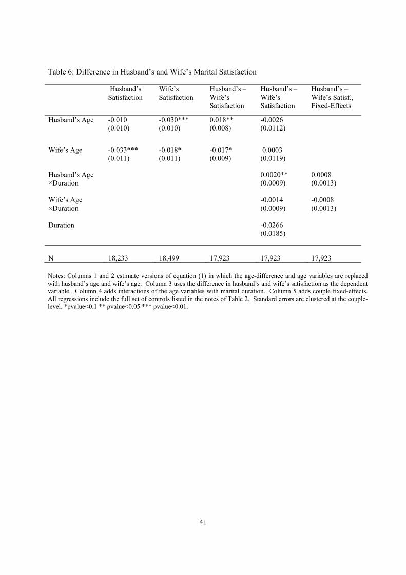
  41

Table 6: Difference in Husband’s and Wife’s Marital Satisfaction

Husband’s Satisfaction

Wife’s Satisfaction

Husband’s – Wife’s Satisfaction

Husband’s –Wife’s Satisfaction

Husband’s –Wife’s Satisf., Fixed-Effects

Husband’s Age -0.010 (0.010)

-0.030*** (0.010)

0.018** (0.008)

-0.0026 (0.0112)

Wife’s Age -0.033*** (0.011)

-0.018* (0.011)

-0.017* (0.009)

0.0003 (0.0119)

Husband’s Age ×Duration

0.0020** (0.0009)

0.0008 (0.0013)

Wife’s Age ×Duration

-0.0014 (0.0009)

-0.0008 (0.0013)

Duration

-0.0266 (0.0185)

N

18,233

18,499

17,923

17,923

17,923

 

Notes: Columns 1 and 2 estimate versions of equation (1) in which the age-difference and age variables are replaced with husband’s age and wife’s age. Column 3 uses the difference in husband’s and wife’s satisfaction as the dependent variable. Column 4 adds interactions of the age variables with marital duration. Column 5 adds couple fixed-effects. All regressions include the full set of controls listed in the notes of Table 2. Standard errors are clustered at the couple-level. *pvalue<0.1 ** pvalue<0.05 *** pvalue<0.01.

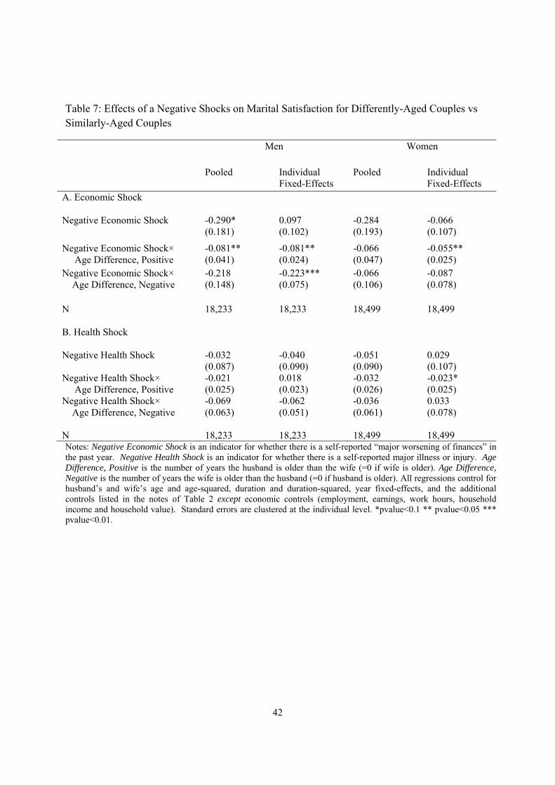
  42

Table 7: Effects of a Negative Shocks on Marital Satisfaction for Differently-Aged Couples vs Similarly-Aged Couples

Men

Women

Pooled Individual Fixed-Effects

Pooled Individual Fixed-Effects

A. Economic Shock Negative Economic Shock

-0.290* (0.181)

0.097 (0.102)

-0.284 (0.193)

-0.066 (0.107)

Negative Economic Shock× Age Difference, Positive

-0.081** (0.041)

-0.081** (0.024)

-0.066 (0.047)

-0.055** (0.025)

Negative Economic Shock× Age Difference, Negative

-0.218 (0.148)

-0.223*** (0.075)

-0.066 (0.106)

-0.087 (0.078)

N

18,233

18,233

18,499

18,499

B. Health Shock Negative Health Shock

-0.032 (0.087)

-0.040 (0.090)

-0.051 (0.090)

0.029 (0.107)

Negative Health Shock× Age Difference, Positive

-0.021 (0.025)

0.018 (0.023)

-0.032 (0.026)

-0.023* (0.025)

Negative Health Shock× Age Difference, Negative

-0.069 (0.063)

-0.062 (0.051)

-0.036 (0.061)

0.033 (0.078)

N

18,233

18,233

18,499

18,499

Notes: Negative Economic Shock is an indicator for whether there is a self-reported “major worsening of finances” in the past year. Negative Health Shock is an indicator for whether there is a self-reported major illness or injury. Age Difference, Positive is the number of years the husband is older than the wife (=0 if wife is older). Age Difference, Negative is the number of years the wife is older than the husband (=0 if husband is older). All regressions control for husband’s and wife’s age and age-squared, duration and duration-squared, year fixed-effects, and the additional controls listed in the notes of Table 2 except economic controls (employment, earnings, work hours, household income and household value). Standard errors are clustered at the individual level. *pvalue<0.1 ** pvalue<0.05 *** pvalue<0.01.