DISCUSSION PAPER SERIES IZA DP No. 10599 David L. Dickinson David Masclet Emmanuel Peterle Discrimination as Favoritism: The Private Benefits and Social Costs of In-group Favoritism in an Experimental Labor Market FEBRUARY 2017
Transcript
Discussion PaPer series
IZA DP No. 10599
David L. DickinsonDavid MascletEmmanuel Peterle
Discrimination as Favoritism: The Private Benefits and Social Costs of In-group Favoritism in an Experimental Labor Market
FebruAry 2017
Any opinions expressed in this paper are those of the author(s) and not those of IZA. Research published in this series may include views on policy, but IZA takes no institutional policy positions. The IZA research network is committed to the IZA Guiding Principles of Research Integrity.The IZA Institute of Labor Economics is an independent economic research institute that conducts research in labor economics and offers evidence-based policy advice on labor market issues. Supported by the Deutsche Post Foundation, IZA runs the world’s largest network of economists, whose research aims to provide answers to the global labor market challenges of our time. Our key objective is to build bridges between academic research, policymakers and society.IZA Discussion Papers often represent preliminary work and are circulated to encourage discussion. Citation of such a paper should account for its provisional character. A revised version may be available directly from the author.
Policy makers have an interest in reducing or eliminating labor market discrimination. In
this laboratory experiment study, we show that employers who favor certain individuals
(who belong to their identity group) are likely to reap benefits in terms of increased effort
from these (presumably) grateful workers who were shown favoritism. Thus, this type of
discrimination (against those not belonging to the employer’s identity group) may benefit
employers in a narrow sense. However, our experimental design also allows unemployed
workers to destroy resources of employers and other employed workers. We find that
when unemployment is caused by favoritism towards others, the unemployed destroy
significantly more resources (i.e., burn others’ payoffs). Our results therefore highlight a
key spillover cost on society of discrimination that employers may fail to take into account.
2
1. INTRODUCTION
Since the publication of Gary Becker’s The Economics of Discrimination in 1957, the subject
of discrimination has been of particular interest to labor economists. The literature on labor
market discrimination is large, and has benefitted from the complementary efforts of empirical
econometric, field experimental, and controlled laboratory studies. In this paper we aim to
contribute to this existing literature by investigating discrimination in a unique experimental
design that can help shed light on both the private incentives and spillover impacts of
discriminatory practices. In other words, there may be instances where favoring one group of
workers over another may privately benefit the firm, but yet generate spillover costs to society.
According to Becker, taste-based discrimination leads to suboptimal recruiting
decisions. Thus, competitive markets should help eliminate this type of employer
discrimination as prejudiced employers face higher production costs. In contrast, other models
have considered that taste-based discrimination is driven by efficiency considerations such as
reduced costs of communication (Lang, 1986; Athey et al, 2000; Efferson et al, 2008; Feng et
al, 2012). Yet another alternative is that employers may benefit from in-group favoritism in
terms of reciprocal effort. Specifically, in-group workers may provide high effort both in
response to in-group employment favoritism as well as in-group wage favoritism. In either
case, this implies that not all taste-based discrimination is detrimental from the perspective of
the firm’s private cost/benefit analysis. In this current paper we attempt to isolate the extent of
reciprocity induced by in group favoritism.
In addition to providing evidence that addresses the issue of favoritism and reciprocity
between in-group employers and workers, our paper’s second objective is to generate unique
data on spillover effects of discrimination/favoritism. Specifically, our experimental design
allows us to measure one type of spillover cost of discrimination on society by allowing
unemployed worker subjects (who may or may not be able to attribute their unemployed status
to in-group favoritism) to destroy resources (i.e., burn money) of others. While there are
limitations to how much laboratory money-burning choices can teach us about true societal
costs like fragmentation and increased conflict, our data may be viewed as providing at least
some evidence of one micro-foundation of increased societal tension and riots. Such costs of
discrimination on society are typically ignored in existing research.
The potential for disgruntled societal groups to engage in costly anti-social behavior
(and, at the extreme, riots) is real. For example, significant costs to society were incurred in
France in 2006 when proposed labor laws upset young workers who viewed the new laws as
3
unfair or discriminatory towards new workers. In Paris alone, more than 500,000 protestors
gathered, and the media coverage showed evidence of explicit societal costs as store fronts were
vandalized and cars torched by a few dozen rioters.1 Even recent civil unrest in the U.S. that is
not specifically connected to labor market outcomes (e.g., the Baltimore riots of 2015) show
the potential societal costs of tension between identity groups (e.g., racial groups) and real or
perceived in-group favoritism. In our experimental design the subjects in our experimental
“society” who are not hired are deemed unemployed, and these subjects are given an
opportunity to destroy resources of others (i.e., what we call “burn money”). Thus, the inclusion
in our design of an avenue for spillover effects to manifest is an important contribution to the
existing literature. In short, while our results document evidence of private benefits to
employers of discriminating against out-group (or favoring in-group) workers, we also find
significant increases in money burning by unemployed workers in our experimental setting,
which highlights that society as a whole has an interest in addressing systematic favoritism.
2. BACKGROUND
Labor market discrimination may exist for a variety of reasons. In Becker’s model,
discrimination in hiring or wages is caused by a ‘taste for discrimination’, which leads the
employer to hire or pay higher wages to members of her/his own group (henceforth, “in-
group”). Other models predict workplace segregation but consider that in-group biases are
driven by efficiency considerations, such as reduced costs of communication (Lang, 1986;
Athey et al., 2000). Communication costs, in general, are lower among individuals with a
common group identity of some sort. This may be a contributing factor in understanding how
in-group favoritism evolves (Efferson et al, 2008; Feng et al., 2012), which may then help
explain segregation of informal networks (Marsden, 1987). In-group networks have been found
to impact hiring decisions (Granovetter 1995; Holzer, 1996; Bayer et al., 2008; Hensvik and
Nordström Skans, 2016; Gee et al, forthcoming). For example, researchers have found that
work places with black supervisors or owners are significantly more likely to employ black
1 For instance, significant costs to society were incurred in France in October and November 2005, when a series
of riots occurred in the French suburbs, involving the burning of cars and several public buildings. The riots
resulted in three deaths of non-rioters many police injuries and nearly 3000 arrests. A state of emergency was
declared on 8 November, later extended for three weeks, and the government announced a crackdown on
immigration. This event was an expression of frustration and real or perceived discrimination on the labor market
from immigrant communities with Arab or otherwise Muslim background.
4
workers (Bates, 1994; Carrington and Troske, 1998; Stoll et al., 2004; Giuliano et al., 2009).
This suggests that in-group favoritism may be key component of the discriminatory outcome.
An alternative to taste-based discrimination is statistical discrimination (Phelps, 1972;
Arrow, 1972). According to this approach, employers have incomplete information about the
worker’s potential performance. Imperfect information arises either because minority groups
emit noisier signals (Phelps, 1972; Aigner and Cain, 1977; Cornell, and Welch, 1996; Pinkston,
2003) or because negative prior beliefs about members of a particular group may become self-
fulfilling in equilibrium (Lundberg and Startz, 1983). In the environment we study, we remove
the potential that discrimination or favoritism results from anything other than group
identification (i.e., no reduced communication costs, no extra productivity information on
workers due to group affiliation, etc). Thus, we view laboratory methods, in this instance, to
be a particularly attractive approach for generating primary data that is relatively free from
confounds typically present in field data.
An exhaustive account of the different types of discrimination is beyond the scope of
this paper, but it is worth noting what laboratory methods have contributed to the study of
discrimination. Examples of laboratory studies aimed at studying the determinants of
discrimination include: Holm, 2000; Anderson and Haupert, 1999; Fershtman and Gneezy,
2001; Fryer et al., 2005; Dickinson and Oaxaca, 2009, 2014; Slonim and Guillen, 2010; Castillo
and Petrie, 2010; Rödin and Özcan, 2011; Falk and Zehnder, 2013; see also Anderson et al.
2006 for a survey). As noted above, laboratory data generation is a methodological alternative
intended to facilitate the ability to identify determinants of discrimination (Giuliano et al., 2009,
is an exception). In general, controlled laboratory environments allow one to isolate a key
variable of interest in an otherwise complicated labor market environment, thus facilitating
causal inference. Laboratory research has shown that statistical discrimination may result from
risk aversion, mistaken stereotypes, incomplete information, or assessment bias (Anderson and
Haupert, 1999; Davis, 1987; Fershtman and Gneezy, 2001; Dickinson and Oaxaca, 2009;
Castillo and Petrie, 2010). A recent laboratory study also found that discrimination based on
statistical differences in worker productivity-types may lead to hiring as well as wage-based
discrimination (Dickinson and Oaxaca, 2014).
Our current focus is the in-group favoritism of workers by employers, where the nature
of group identity carries no relevant information content at all. As such, in-group preference
or the expectation of reciprocity by workers are the only identifiable reason to show favoritism
by group identity in such instances. Thus, a final relevant stream of literature worth noting
involves laboratory research on group identity formation and its effects on behavior. Research
5
has found that the more salient the in-group membership status, the larger the impact on
behavior (Charness et al, 2007). Our use of a gift-exchange environment to study employer-
worker decisions is related to cooperation and reciprocity concerns. Eckel and Grossman (2005)
reported that group identification increased cooperation in a public goods game, while Chen
and Li (2009) found that in-group members were more forgiving and more interested in
maximizing welfare of their particular group.2 Other recent research also reports significant in-
group favoritism (e.g. Chen and Chen, 2011; Chen et al, 2014; Currarini and Mengel, 2016).
Of particular relevant to our work is the Chen and Chen (2011) result that effort coordination
increased to high levels when group identity was made more salient. Their result suggests
positive reciprocity by in-group workers in gift-exchange effort environments, which would
make employers rationally choose to favor in-group workers (i.e., discriminate against out-
group workers). Our experimental design will highlight how we intend to identify the spillover
effect on society that may result from such privately rational favoritism.
3. EXPERIMENT DESIGN
3.1 Preliminary Phase—Social Preference Elicitation and Group Identity Induction
Before the main hiring and effort experiment, subjects participated in a 2-part preliminary
phase. In the first part, we use an existing procedure to generate common measures of social
preferences (Blanco et al, 2011). Specifically, a measure of disadvantageous inequality aversion
(i.e., “envy”) is derived from ultimatum game responder choices, and a modified dictator game
is used to generate a measure of advantageous inequality aversion (called “guilt” by Blanco et
al, 2011, but can be considered a proxy for altruism. See instructions in Appendix A for further
detail on these social preference tasks).3 Decisions in the social preference elicitation tasks were
incentivized4, but participants were not informed of the preliminary task outcome until the end
2 Others have shown that trust may increase in groups, which points to another potential benefit of showing
preferences towards one’s own group (Glaeser at al, 2000; Eckel and Wilson, 2004; Bernhard et al, 2006; Goette
et al., 2006; Falk and Zehnder, 2007; Buchan et al., 2008; Fiedler et al., 2011). This points to another rationale
for discrimination, namely the increase social capital within the group. 3 Inequality aversion stipulates that individuals care about the distribution of monetary payoffs in addition to their
own payoff. Specifically, an inequality averse individual prefers equal monetary payoffs for all players, though
some may have a differential aversion to inequality depending on whether it benefits (advantageous inequality) or
harms oneself (disadvantageous inequality). Models of inequality aversion were first proposed by Bolton (1991)
and refined by Fehr and Schmidt (1999) and Bolton and Ockenfels (2000). Using the Blanco et al (2011) tasks,
we calculate the and parameters for each subject described in Fehr and Schmidt (1999) as measures of
disadvantageous and advantageous inequality, respectively. 4 More specifically, one row of the payoff matrix is randomly selected from each game for payoff.
6
of the experiment in order to avoid wealth effects. Furthermore, the lack of context in these
preliminary tasks helped avoid the potential for behavioral spillovers into the main experiment.
During a second part of this preliminary phase, we induce group identities. These group
identities are a relevant variable of interest in our design. Each experimental “society” consists
of 8 subjects divided into two groups of 4 subjects each. Groups are formed based on similarity
of choices in a movie preference task— drama or comedy film were the options given to
subjects. Then we increase the saliency of group identity by asking matched participants to
choose a group name from among a predefined list of sea/ocean name options to represent the
group’s “identity” (e.g., group “Atlantic”, group “Baltic”).5 Our choice to induce otherwise
meaningless group identities rather than use subjects’ natural identities (e.g. gender, ethnicity
or social background) was intended to increase control over the group assignments and limit
selection concerns in the data. Thus, throughout the experiment subjects are assigned to a
society that includes two different identity-groups.
3.2 Main Experiment Phase
An experimental “society” consists of a group of 8 subjects: 2 employers, 4 workers, and 2
unemployed. The experimental treatments consist of several stages involving distinct decisions.
In Stage 1 (present only in half the treatments), each subject makes decisions in the role of an
employer who must hire two workers who will each make an effort choice affecting the
employer’s monetary payoff (e.g. Sutter and Weck-Hannemann, 2003). As a potential
employer, subjects rank the other 7 members of his/her society from most (rank=1) to least
(rank=7) preferred. Information on the group identity of each subject is common knowledge
when making one’s ranking decisions, and these rankings are then used to form firms within
the society for some treatments.6 Subjects were fully aware that these rankings would be
binding should the subject be randomly assigned as an employer in the following stage of the
experiment.
Once all employers submit their rankings, firms composed of an employer and two
employees are formed using a two-step mechanism similar to the one suggested by
Bogomolnaia and Jackson (2002) (see also Castillo and Petrie, 2010). In step one, the first
5 Group name choice was accomplished using a 3-minute chat feature in the computer interface such that
participants could only interact with other members of their identity group. It was forbidden to reveal one’s true
identity. At the end of the 3-minute chat, group name was selected by majority rule. 6 Specifically, subjects are told that those assigned a preferred rank are more likely to be recruited as a worker
for that subject, should he/she be randomly assigned as an employer.
7
employer (called A1) is randomly chosen by the computer and is matched with her/his two
preferred employees based on her/his ranking. Thus, a first firm is formed with this employer
and her/his two best ranked workers (called worker B1 and B2). In a second step, the second
employer (called A2) is matched with her/his two most preferred employees (called B3 and B4)
from among the remaining four participants who have not yet been assigned to the first
employer in step one. The two participants not assigned to a firm are assigned the role of
unemployed workers (unemployed worker C1 and unemployed worker C2 respectively). The
two unemployed workers in each group do not take part in Stage 2 of the game and receive a
fixed payment of 5 EMU (Experimental Monetary Units), which is analogous to unemployment
insurance.
The second experimental stage (Stage 2), which is present in all treatments, consists of a
gift-exchange game between employers and their respective workers. Employers assign
(potentially unequal) wages to the workers of their respective firm. Wage options are w = 16 or
w = 32, for the employer. We use the strategy method to elicit employers’ decision for each
potential identity-group composition of the firm. Workers then choose an integer level effort e
∈ [1, 4] for each potential wage distribution within the firm and for both of the possible
employer identity-groups. Unemployed participants do not participate to this stage. Employer
profits are a function of the two employee effort levels e1 , e2 and the wages paid to each
employee, w1, w2 according to the following function:
(1) (e1,e2,w1,w2) = 32 (e1 + e2) – w1 – w2.
Our examination of societal spill-over costs involves the final Stage 3 in all treatments,
which allows unemployed participants take part in a money-burning game. Here, unemployed
workers can either target specific individuals in the society (at a relatively high cost — 1 EMU
paid burns 5 EMU of a specific target individual) or burn money of both employers and workers
without distinction (for a relatively low cost — 1 EMU paid burns 2 EMUs of other employer
and worker payoff).7 This Stage 3 money burning game allows unemployed workers to express
their dissatisfaction in a way that is costly to the society, which we consider important in
evaluating the overall impact of discrimination or favoritism in the labor market.
7 A subject choosing the “burn with no distinction” option was not allowed to individually target subjects for additional money burning.
8
3.3 Experimental Treatments
We implement four treatments in a 2x2 factorial design. The first factor varied is the process
of worker employment assignments in Stage 1 of the main experiment. In the Ranking
treatments, subjects take part in the Stage 1 rankings described above. In contrast, in the
Random treatments Stage 1 randomly assigns subject roles. The comparison of these two
treatments identifies how hiring discrimination or favoritism affects individual behaviors of
employed and non-employed participants. The second factor in our 2x2 design varies the cost
of effort of subjects. In the Homogeneous Cost treatments, all workers face the same marginal
cost of 5 EMU for each effort unit. The total effort cost function for all subjects is:
(2) C(e)=5e-5
In the Heterogeneous Cost treatments, a society is divided in highly productive (low effort
cost, C(e)=3e-3) and low productivity (high effort cost, C(e)=5e-5) workers. By comparing
individual decisions in Homogeneous and Heterogeneous Cost treatments, we investigate
whether productive individuals who face discrimination are willing to retaliate by providing
less effort (if employed) or burning money (if unemployed). Recall that unemployed workers
earn a fixed payoff of 5 EMU, while the range of possible payoffs to workers is [1,32] EMU
for high cost of effort workers, and [7,32] EMU for low cost of effort workers. The range of
possible payoffs for the employers are [0,224] EMU.
3.4 Procedures and Parameters
The experiment consists of 8 sessions conducted at the CREM-CNRS (LABEX-EM) institute
of the department of Economics of the University of Rennes 1 in France. Summary information
about the 8 sessions is shown in Table 1.
Table 1. Experimental Sessions
Sessions Treatment # Participants
1 ; 2 Homogeneous Ranking 48
3 ; 4 Homogeneous Random 48
5 ; 6 Heterogeneous Ranking 48
7 ; 8 Heterogeneous Random 48
Total number of participants: 192
A total of 192 undergraduate students in management, economics, law, medicine, arts and
sciences were recruited via the ORSEE software (Greiner, 2004). Participants earned on
average 15.52€, including a show-up fee of 5€. During the experiment, all payments were
9
expressed in experimental currency units (EMU), and are converted to Euros at a predetermined
conversion rate of 5 EMU = 1€. Some of the participants may have participated in experiments
before but, to our knowledge, none had experience in any experiment similar to ours. No
individual participated in more than one session of this study.8 On average, sessions lasted about
75 minutes including instructions and payment of participants. The experiment was
computerized using the Z-tree software package (Fischbacher, 2007).
3.5 Hypotheses
Consider first the hiring decisions in the Ranking treatments. If participants do not have
discriminatory or favoritism based preferences, they should view group identities as irrelevant
when assigning ranks — they should assign ranks randomly. However, one may conjecture that
employers may have distaste for hiring people not belonging to their own group (Becker, 1957;
Lang, 1986; Athey et al., 2000), or a preference for hiring in-group members as research has
documented (Bouckaert and Dhaene, 2004).9 In addition, one may also reasonably expect that
individuals may be more likely to hire in-group individuals if they anticipate reciprocal higher
effort in the gift exchange game (i.e., higher effort than out-group workers). Note, however,
that this in-group favoritism may be offset in the Heterogeneous Ranking treatment if
employers care more about high productivity (i.e., low effort cost) workers than they care about
group identity. Our conjecture is summarized below in H1:
H1a: In Ranking treatments, preferred ranks will be assigned to in-group subjects.
H1b: In-group favoritism in rankings will be lower in Ranking Heterogeneous compared to
Ranking Homogeneous due to worker productivity differences.
Our second set of hypotheses describe the expected impact of in-group favoritism (or out-group
discrimination) on wage choices. The fact that there may be a trade-off between hiring and
wage discrimination is also quite intuitive and was found by Dickinson and Oaxaca (2014).
H2a: Across all treatments, wages offered to in-group subjects will be higher than wages
offered to out-group subjects.
H2b: Wage favoritism towards in-group subjects will be higher in the Random treatments,
where there is not an additional opportunity to show favoritism in hiring.
8 The ORSEE recruitment software allows us to clearly identify students who have already participated to a similar
game. However, we acknowledge that we cannot totally rule out the fact that they might have played a similar
game in another university/institution, though we consider this very unlikely. 9In-group favoritism and out-group discrimination have been very robust findings in the social psychology
literature (Tajfel et al. 1971; Billig and Tajfel, 1973; Turner and Brown, 1978; Vaughan et al. 1981; Diehl, 1988;
Pratto and Shih, 2000).
10
These first two sets of hypotheses focus on in-group favoritism impact on the dimensions of
subject rankings and wage offerings. The remaining two sets of hypotheses focus on positive
and negative reciprocity effects of the workers (hired and unemployed). A large body of
research documents positive reciprocity in numerous settings (including gift exchange
experiments, see Fehr et al, 1997), but recent research also finds that individuals display more
positive reciprocity towards in-group members (Chen and Li, 2009). This leads to hypotheses
H3:
H3a: In-group workers will choose higher effort levels than out-group workers.
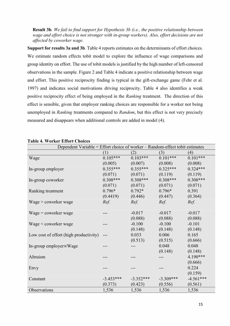
H3b: The wage-effort reciprocity effect will be stronger between in-group employer-
workers.
Finally, our last hypothesis stems from the assumption that being unemployed creates
dissatisfaction, which is heightened when the unemployment is the result of the intentional
ranking choices in the Ranking treatments. Furthermore, money burning should be
disproportionately directed towards employers in Ranking treatments given the intentionality
of rankings that lead to unemployment. And finally, We consider that money burning may be
higher in societies with heterogeneous productivity across workers. In this case, employed
workers who are low productivity (i.e., high cost of effort) may be a particular target for money
burning given that employers would not reasonably hire a low productivity worker unless
favoring one’s group identity more strongly than one’s productivity (and profit) potential.
H4a: Money burning will be higher in Ranking compared to Random treatments.
H4b: Money burning in Ranking treatments will more often target employers than
individuals in general.
H4c: Money burning will be higher in Heterogeneous treatments and will more often
target low productivity (employed) workers, rather than high productivity workers.
4. RESULTS
We first investigate whether participants show favoritism towards in-group members (i.e.,
discriminate) in hiring, wage and effort decisions. These outcome measures inform our
understanding of the private incentives firms may have to show favoritism. After analysis of
the employer and worker decisions, we then investigate the social costs of favoritism in the
form of unemployed worker money-burning choices.
11
4.1 Discrimination and its Rationale
4.1.1. In-group favoritism in hiring
Our data show that participants tend to rank in-group members more favorably (i.e., lower
ranks). In the Homogeneous Ranking treatment, in-group members are assigned an average rank
of 2.35 whereas out-group members are assigned an average rank of 5.24 (Wilcoxon signed-
rank, p<0.001). The additional information on productivity heterogeneity in the Heterogeneous
Ranking treatment lowers this gap—the average in-group ranking is 2.98 compared to 4.77 for
out-group members, which is a significantly reduced gap compared to Homogenous Ranking
gap (Wilcoxon Mann-Whitney, p<0.001). However, preferential ranking of in-group members
remains significant (Wilcoxon signed-rank, p<0.001). These findings support both hypotheses
H1a and H1b.
Result 1a. In Ranking treatments, in-group members are ranked significantly better, on
average.
Result 1b. The extent of in-group favoritism is lower - but still existing – in Heterogeneous
treatments (i.e., some out-group members have lower effort costs than some in-group
members, which makes them more desirable workers to the employer)
Support for results 1a and 1b. Table 2 reports the results of rank-ordered logit models (Beggs
et al., 1981) on the determinants of the employer’s ranking decision. The dependent variable
Rankij corresponds to the rank employer i assigns to each potential job candidate j. The
independent variables include candidate’s identity group, as well as a control for candidate’s
productivity in the heterogeneous ranking treatment (column 3). All models indicate that in-
group members are ranked significantly better than out-group members (i.e., lower rank value).
Model (3) of Table 2 indicates that low productivity (i.e., high effort-cost) workers are ranked
worse than high productivity workers, holding identity group constant.
Table 2. Ranking Decisions
Rank attributed by player i to player j – Rank-Ordered Logit estimates
(1)
Pooled
regression
(2)
Homogenous
Treatment
(3)
Heterogenous
Treatment
Player j is from same group -1.725***
(0.126)
-2.604***
(0.244)
-1.210***
(0.153)
Player j has high effort cost --- --- 0.394**
(0.154)
Observations 672 336 336
12
Number of individuals 96 48 48 Notes: Standard deviations are displayed in parentheses. Lower ranks are preferred ranks.
11 We acknowledge that there are multiple reasons why individuals may riot. It is because we find evidence that
the Ranking treatment leads to more employer-targeted money burning that we can claim that our results identify
a spillover effect directly linked to favoritism (as opposed to the general discontent money burning that may
result from labor productivity inequality we induce in Heterogenous treatments).
21
5. CONCLUSIONS
We present a new experimental design that permits us to investigate not only the private
incentives to show favoritism (or discriminate), but it also allows us to evaluate a type of
spillover costs on society. Consistent with previous findings, we find that the conditions for the
occurrence of discrimination are rather weak (Holm, 2000). Our lab design generates
discriminatory treatment of individuals not associated with one’s group (i.e., out-group
members) under conditions of a contrived laboratory-induced group identity. An alternative
perspective is to view this as favoritism towards in-group members. Whatever the label, a key
objective of this paper is to highlight that favoritism based purely on group identity (i.e., no
impact on costs or information from showing such favoritism) can be privately beneficial to an
employer, and yet produce spillover costs to society from discontent among excluded workers.
Importantly, this discontent will express itself in one way or another (as it always does), and
we focus on one particular channel for expressing discontent that yields insights into issues
relevant to society.
We opted for experimental data generation to more cleanly identify favoritism based purely on
group identity, as well as to channel any discontent into a limited set of consequential options.
In field data, hiring based on social networks likely allows for reduced communication costs or
provides the employer with valuable information on a candidate, both of which present a
confound in assessing favoritism for pure group identity reasons. Unemployed worker
discontent in the field can also be expressed in numerous ways, which are often not quantifiable
or always even identifiable. As such, for our particular research question the laboratory offers
an advantage over field data, and makes possible the identification of causal favoritism effects
that are difficult to identify in the naturally occurring economy.
We report three key findings: First, we find evidence that even a weakly constructed common
group identity becomes a source of favoritism both at the hiring stage and in wage offers. While
this documents multiple dimensions on which discrimination may operate, even in a laboratory
environment (see Dickinson and Oaxaca, 2014), the potential for positive reciprocity towards
employers by those hired and/or offered high wages may actually imply that such in-group
favoritism may be in the monetary payoff interest of the employer. Second, subjects generally
reciprocate high wage offers with higher effort choices. Importantly, our data confirm that
workers make higher effort choices for in-group employers than for out-group employers, and
this effect is largely the same across treatments. This finding suggests that employers should
22
rationally prefer in-group workers over out-group workers, all else equal. Finally, while there
may be some evidence that in-group favoritism benefits employers, we considered the spillover
costs on society of unemployed workers burning resources. We find evidence of significant
money burning when productivity inequality exists in society, and also when employment
discrimination is more present. Thus, labor market favoritism that plausibly produces discontent
is likely an important micro-foundation of more significant societal costs.
Our study is not without its limitations, which may offer avenues to extend this research. For
example, our use the strategy method was a design choice intended to maximize the data
generation from a fixed set of subjects. One might argue that data from contingency decisions
may differ from choice data elicited from a single decision scenario. We also highlight the
limited number of observations on money burning decisions due to the somewhat limited
(n=48) set of unemployed subjects in our design. A study focused on the money burning costs
may choose a design with a larger set of unemployed subjects relative to employed. The
sensitivity of our results to elements such as these are ultimately empirical questions that can
be explored in future research. Nevertheless, we feel that our evidence for favoritism spillover
costs, even in a stylized laboratory environment, highlights their importance in understanding
the full impact of discrimination/favoritism in labor markets. It also highlights an important
argument for why discrimination/favoritism is undesirable for society as a whole.
23
References
Aigner, D. J., & Cain, G. G. (1977). Statistical theories of discrimination in labor markets. Industrial and Labor Relations Review, 30(2), 175-187.
Anderson, D. M., & Haupert, M. J. (1999). Employment and statistical discrimination: A hands-on experiment. The Journal of Economics, 25(1), 85-102.
Anderson, L., Fryer, R., & Holt, C. (2006). Discrimination: experimental evidence from psychology and economics. Handbook on the Economics of Discrimination, 97-118.
Arrow, Kenneth J. (1972). Models of job discrimination. In Racial discrimination in economic life, edited by A.H. Pascal. Lexington, MA: D.C. Heath, 83-102.
Athey, S., Avery, C., & Zemsky, P. (2000). Mentoring and Diversity. American Economic Review, 90(4), 765-786.
Bates, T. (1994). Utilization of minority employees in small business: A comparison of nonminority and black-owned urban enterprises. The Review of Black Political Economy, 23(1), 113-121.
Bayer, P., Ross, S. L., & Topa, G. (2008). Place of work and place of residence: Informal hiring networks and labor market outcomes. Journal of Political Economy, 116(6), 1150-1196.
Becker Gary, S. (1957). The economics of discrimination. Chicago, University of Chicago Press.
Beggs, S., Cardell, S., & Hausman, J. (1981). Assessing the potential demand for electric cars. Journal of Econometrics, 17(1), 1-19.
Bernhard, H., Fehr, E., & Fischbacher, U. (2006). Group affiliation and altruistic norm enforcement. The American Economic Review, 96(2), 217-221.
Billig, M., & Tajfel, H. (1973). Social categorization and similarity in intergroup behaviour. European Journal of Social Psychology, 3(1), 27-52.
Blanco, M., Engelmann, D., & Normann, H. T. (2011). A within-subject analysis of other-regarding preferences. Games and Economic Behavior, 72(2), 321-338.
Bogomolnaia, A., & Jackson, M. O. (2002). The stability of hedonic coalition structures. Games and Economic Behavior, 38(2), 201-230.
Bolton, G. E. (1991). A comparative model of bargaining: Theory and evidence. The American Economic Review, 81(5), 1096-1136.
Bolton, G. E., & Ockenfels, A. (2000). ERC: A theory of equity, reciprocity, and competition. The American Economic Review, 90(1), 166-193.
Bouckaert, J., & Dhaene, G. (2004). Inter-ethnic trust and reciprocity: results of an experiment with small businessmen. European Journal of Political Economy, 20(4), 869-886.
Buchan, N. R., Croson, R. T., & Solnick, S. (2008). Trust and gender: An examination of behavior and beliefs in the Investment Game. Journal of Economic Behavior & Organization, 68(3), 466-476.
Carrington, W. J., & Troske, K. R. (1998). Interfirm segregation and the black/white wage gap. Journal of Labor Economics, 16(2), 231-260.
Castillo, M., & Petrie, R. (2010). Discrimination in the lab: Does information trump appearance?. Games and Economic Behavior, 68(1), 50-59.
Charness, G., Rigotti, L., & Rustichini, A. (2007). Individual behavior and group membership. The American Economic Review, 97(4), 1340-1352.
Chen, R., & Chen, Y. (2011). The potential of social identity for equilibrium selection. The American Economic Review, 101(6), 2562-2589.
Chen, Y., & Li, S. X. (2009). Group identity and social preferences. The American Economic Review, 99(1), 431-457.
Chen, Y., Li, S. X., Liu, T. X., & Shih, M. (2014). Which hat to wear? Impact of natural identities on coordination and cooperation. Games and Economic Behavior, 84, 58-86.
24
Cornell, B., & Welch, I. (1996). Culture, information, and screening discrimination. Journal of Political Economy, 104(3), 542-571.
Currarini, S., & Mengel, F. (2016). Identity, homophily and in-group bias. European Economic Review, 90, 40-55.
Davis, D. D. (1987). Maximal quality selection and discrimination in employment. Journal of Economic Behavior & Organization, 8(1), 97-112.
Dickinson, D. L., & Oaxaca, R. L. (2009). Statistical discrimination in labor markets: An experimental analysis. Southern Economic Journal, 76(1), 16-31.
Dickinson, D. L., & Oaxaca, R. L. (2014). Wages, employment, and statistical discrimination: Evidence from the laboratory. Economic Inquiry, 52(4), 1380-1391.
Diehl, M. (1988). Social identity and minimal groups: The effects of interpersonal and intergroup attitudinal similarity on intergroup discrimination. British Journal of Social Psychology, 27(4), 289-300.
Eckel, C. C., & Grossman, P. J. (2005). Managing diversity by creating team identity. Journal of Economic Behavior & Organization, 58(3), 371-392.
Eckel, C. C., & Wilson, R. K. (2004). Is trust a risky decision?. Journal of Economic Behavior & Organization, 55(4), 447-465.
Efferson, C., Lalive, R., & Fehr, E. (2008). The coevolution of cultural groups and ingroup favoritism. Science, 321(5897), 1844-1849.
Falk, A., & Zehnder, C. (2013). A city-wide experiment on trust discrimination. Journal of Public Economics, 100, 15-27.
Fehr, E., & Schmidt, K. M. (1999). A theory of fairness, competition, and cooperation. The Quarterly Journal of Economics, 114(3), 817-868.
Fu, F., Tarnita, C. E., Christakis, N. A., Wang, L., Rand, D. G., & Nowak, M. A. (2012). Evolution of in-group favoritism. Scientific Reports, 2, 460.
Fehr, E., Gächter, S., & Kirchsteiger, G. (1997). Reciprocity as a contract enforcement device: Experimental evidence. Econometrica: journal of the Econometric Society, 833-860.
Fershtman, C., & Gneezy, U. (2001). Discrimination in a segmented society: An experimental approach. The Quarterly Journal of Economics, 116(1), 351-377.
Fischbacher, U. (2007). z-Tree: Zurich toolbox for ready-made economic experiments. Experimental Economics, 10(2), 171-178.
Fiedler, M., Haruvy, E., & Li, S. X. (2011). Social distance in a virtual world experiment. Games and Economic Behavior, 72(2), 400-426.
Fryer, R. G., Goeree, J. K., & Holt, C. A. (2005). Experience-based discrimination: Classroom games. The Journal of Economic Education, 36(2), 160-170.
Gee, L. K., Jones, J. J., & Burke, M. (Forthcoming). Networks and Labor Markets: How Strong Ties
Relate to the Labor Market Using Facebook’s Social Network. Journal of Labor Economics.
Giuliano, L., Levine, D. I., & Leonard, J. (2009). Manager race and the race of new hires. Journal of Labor Economics, 27(4), 589-631.
Glaeser, E. L., Laibson, D. I., Scheinkman, J. A., & Soutter, C. L. (2000). Measuring trust. The Quarterly Journal of Economics, 115(3), 811-846.
Goette, L., Huffman, D., & Meier, S. (2006). The impact of group membership on cooperation and norm enforcement: Evidence using Random assignment to real social groups. The American Economic Review, 96(2), 212-216.
Granovetter, Mark. (1995). Getting a job: A study of contacts and careers. 2nd ed. Chicago: University of Chicago Press.
Greiner, B. (2004). An Online Recruitment System for Economic Experiments. University Library of Munich, Germany.
25
Hensvik, L., & Skans, O. N. (2016). Social networks, employee selection, and labor market outcomes. Journal of Labor Economics, 34(4), 825-867.
Holm, H. J. (2000). Gender-based focal points. Games and Economic Behavior, 32(2), 292-314.
Holzer, Harry J. (1996). What employers want: Job prospects for less educated workers. New York:
Russell Sage Foundation.
Lang, K. (1986). A language theory of discrimination. The Quarterly Journal of Economics, 101(2), 363-382.
Lundberg, S. J., & Startz, R. (1983). Private discrimination and social intervention in competitive labor market. The American Economic Review, 73(3), 340-347.
Marsden, P. V. (1987). Core discussion networks of Americans. American Sociological Review, 122-131.
Phelps, E. S. (1972). The statistical theory of racism and sexism. The American Economic Review, 62(4), 659-661.
Pinkston, J. C. (2003). Screening discrimination and the determinants of wages. Labour Economics, 10(6), 643-658.
Pratto, F., & Shih, M. (2000). Social dominance orientation and group context in implicit group prejudice. Psychological Science, 11(6), 515-518.
Rödin, M., & Özcan, G. (2011). Is It How You Look or Speak That Matters?-An Experimental Study Exploring the Mechanisms of Ethnic Discrimination (No. 2011: 3). Stockholm University Linnaeus Center for Integration Studies-SULCIS.
Slonim, R., & Guillen, P. (2010). Gender selection discrimination: Evidence from a trust game. Journal of Economic Behavior & Organization, 76(2), 385-405.
Stoll, M. A., Raphael, S., & Holzer, H. J. (2004). Black Job Applicants and the Hiring Officer's Race. Industrial and Labor Relations Review, 57(2), 267-287.
Sutter, M., & Weck-Hannemann, H. (2003). Taxation and the Veil of Ignorance–A real effort experiment on the Laffer curve. Public Choice, 115(1-2), 217-240.
Tajfel, H., Billig, M. G., Bundy, R. P., & Flament, C. (1971). Social categorization and intergroup behaviour. European Journal of Social Psychology, 1(2), 149-178.
Turner, J., and R. Brown. (1978). Social status, cognitive alternatives and intergroup relations. Differentiation between social groups: Studies in the social psychology of intergroup relations, 201-234.
Vaughan, G. M., Tajfel, H., & Williams, J. (1981). Bias in reward allocation in an intergroup and an interpersonal context. Social Psychology Quarterly, 37-42.
26
Appendix A : Instructions
Instructions are translated from French. The instruction set presented here corresponds to the Heterogeneous
Ranking treatment, which is the most complete treatment of our experiment. Sets of instructions for other
treatments are available upon request.
General instructions
You are now taking part in an economic experiment. You will take several decisions which are described in this
instruction sheet. The instructions are simple. Following them carefully will allow you to earn a considerable
amount of money.
Your earnings depend on your own decisions and in some case on the decisions of other participants. It is very
important that you read these instructions carefully. Your final earnings will be the sum of what you earn in each
game. During the experiment your entire earnings will be calculated in ECU (Experimental Currency Units). At
the end of the experiment the total amount of ECU you have earned will be converted to euro at the following rate:
5 ECU = €1. Note that you receive a show-up fee of €5 for your participation to the experiment. We guarantee
anonymity for every decision you make.
Game 1
Game 1 includes two steps.
Step 1.
You are randomly matched with another participant in the room. You will receive an endowment of 20 ECU. You
must choose how to distribute this endowment between yourself and the other participant. More specifically, you
can decide an amount (integer number) to offer to the participant you are matched with.
Please note that in the second step, the participant you are matched with will choose whether to accept or to reject
the amount you offer. If the other participant accepts your offer, you will both receive the selected earnings. If the
other participant declines your offer, you will both earn nothing in game 1.
Step 2.
A new random draw will match you with a participant in the room. Just like you, this participant made a decision
in the first step. He received an endowment of 20 ECU and chose an amount to offer you. You are not informed
of this decision. In step 2, you have to declare, for each amount that could have been offered to you, whether to
accept or reject the offer. The decision screen will be presented as follows:
27
If you accept the offer, you will both receive the selected earnings.
If you decline the offer, you will both earn nothing in game 1.
Your earnings in game 1 are the sum of the amount you kept in the first step (if your offer was accepted) and the
amount you were offered in the second step (if you accepted the offer).
Game 2
In game 2, you are randomly matched with a participant in the room. You must select a payoff distribution that
will apply to this participant and yourself. At the same time, another participant selects a payoff distribution that
will apply to you and him/her.
You must make a decision for each line of the following table. All lines represent a different choice between a
payoff distribution A and a payoff distribution B. You must indicate for each line which payoff distribution you
would like to see implemented. The decision screen will appear as follows:
The payoff distribution is represented in brackets. The first figure corresponds to your own payoff, as a decision
maker. The second figure corresponds to the payoff of the player with whom you are matched. For instance, the
distribution (20 ; 0) means “you earn 20 ECU and the other participant earns 0 ECU”. The distribution (6 ; 6)
means “you earn 6 ECU and the other participant earns 6 ECU”.
Once your decision is made, the computer will randomly select a line. It is your decision on that specific line that
will be used to compute your earnings.
Your earnings in game 2 are the sum of the amount you decided to attribute to yourself, and the amount you
received from another participant who played game 2 at the same time and was matched with you. You will receive
information of your payoff at the end of the experiment only.
Game 3
A questionnaire will appear on your screen. You have to honestly answer to the questions. Your answers to those
questions will not affect your earnings, nor will they affect the actions you will undertake in the following games
of the experiment. Furthermore, please recall that your answers are anonymous and will not be associated with
your name. Once the questionnaire is over; we will hand you new instructions.
28
Game 4
The answers you provided to the previous questionnaire have been used to match you with three other participants
in the room. Together you form a group of four participants. Over the course of the experiment, you will stay in
this four-persons group. The three participants you have been matched with are the ones whose answers to the
questionnaire are the most similar to yours. In other words, you are matched in the group of four participants that
corresponds to you the most, based on the questions that have been asked to you previously. Over the course of
the experiment, you will interact with the participants of your own group, but also with the participants of another
group that has been created according to the same process. Therefore, all interactions you will undertake during
the rest of the experiment will always be with the same seven participants (three from your own group and four
from the other group).
In game 4, you collectively choose a name for your group. This name will be used until the end of the experiment
to designate your group. The choice of this name does not affect your future earnings nor the choices you will
make in the future. The name of your group will be chosen via majority voting, from among a predefined list of
five names which will be displayed on your screen. The discussion process will be as follows:
In a first step, you will receive information on the five group names you can choose from. Then, you will have 180
seconds in a chat room discussion to reach an agreement on the name to choose. It is strictly forbidden to reveal
or give any clue on your real identity in the chat room. If you do not respect this restriction, you will be excluded
from the experiment and its payments. Following this discussion, each member of the group votes individually. If
the majority of participants voted for the same name, this name will be assigned to your group for the rest of the
experiment. If no majority is reached, members of your group will vote a second time. If no majority is reached
from this second vote, a random name will be assigned to your group. Game 5
Game 5 includes two steps.
Step 1
In the first step, you rank by order of preference the seven other participants with whom you interact. This ranking
can later be used to form teams. At the end of the first step, a role will randomly be assigned to you. You can be
either employer, worker, or unemployed.
In game 5, all participant will randomly be assigned a characteristic: high cost of effort or low cost of effort. This
characteristic will affect the participants in the role of worker in step 2 of the game.
Your first decision in game 5 will be taken as a potential employer. You will rank the seven other participants by
order of preferences. This ranking will be used to define which workers you would want to recruit in the following
of the game. Your chance to hire the participant is the highest for the participant you rank at the first position and
the lowest for the participant you rank at the seventh position.
A screenshot of your decision screen is provided in the next page of these instructions.
Information regarding participant’s group and participant’s cost of effort will be displayed on the decision screen.
Participants can be members of your own group, or members of the other group. To attribute a rank, you have to
type the letter corresponding to the participant on the right panel of the screen. You cannot enter the same letter
twice. The ranking must be complete. If you make any mistake in the ranking, you will be alerted and you will
have to enter the ranking anew.
Once every participant has declared his/her preference ranking, the computer will assign roles according to the
following rule:
A first participant is randomly selected and is assigned the role of employer.
The two participants at the top of the ranking of this employer will join his/her team, and be assigned the
role of worker.
A new participant, among the remaining ones, will be randomly selected and assigned the role of
employer. The two participants at the top of the ranking of this employer (among remaining participants) will join
his/her team, and assigned the role of worker.
The two participants who have not been assigned the role of employer or worker will be unemployed for
the rest of the experiment.
29
Important: If you are assigned the role of employer, your ranking will be used to match two workers in your team.
You should therefore pay attention when declaring this ranking.
Step 2
Step 2 begins when roles have been assigned to every participant in the room. Your role (employer, worker or
unemployed) will determine the actions you can undertake in step 2. Here is a summary of the actions that will be
undertaken (further detail are given in the following of the instructions).
Employers will decide a wage (16 ECU or 32 ECU) to offer each worker with whom he/she is matched.
Workers will decide on a level of effort (1, 2, 3 or 4). This level of effort affects both workers’ and
employer’s earnings.
Participants in the role of unemployed do not make any decision in this game.
If you are an employer
You have been matched with two workers. You have to decide a wage to offer each of these workers. This wage
can be 16 ECU or 32 ECU. The sum of the wages you assign will be withdrawn from your final profits.
When making this decision, you will not be informed of the exact identity of the workers you have been matched
with. For that reason, you must assign wages for every possible situation. Your decisions will be made in a simple
table. All lines correspond to a different situation, described in the first column. At every line, you must make two
decisions: what wage to pay worker 1, and what wage to pay worker 2.
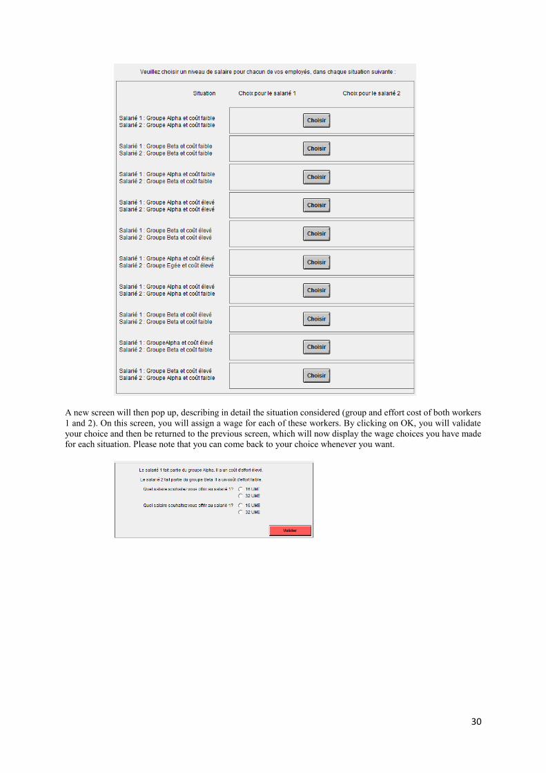
First, you must click on the button “choose”, available at every line of the table (see screenshot below).
30
A new screen will then pop up, describing in detail the situation considered (group and effort cost of both workers
1 and 2). On this screen, you will assign a wage for each of these workers. By clicking on OK, you will validate
your choice and then be returned to the previous screen, which will now display the wage choices you have made
for each situation. Please note that you can come back to your choice whenever you want.
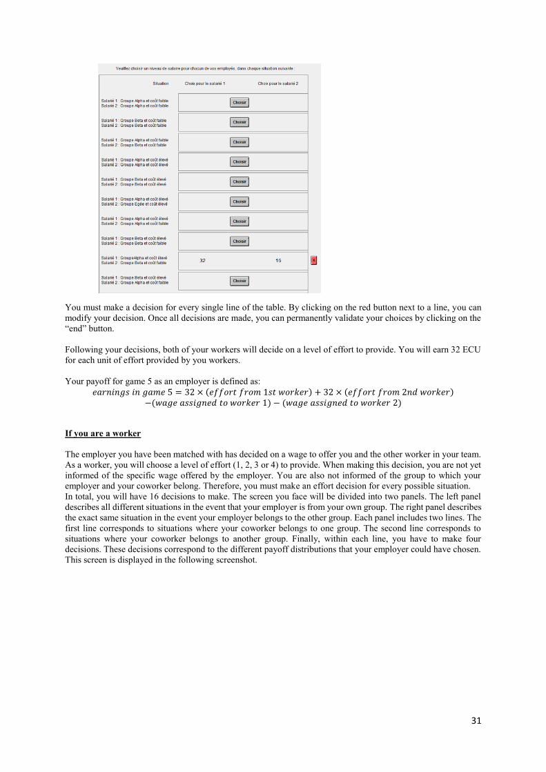
31
You must make a decision for every single line of the table. By clicking on the red button next to a line, you can
modify your decision. Once all decisions are made, you can permanently validate your choices by clicking on the
“end” button.
Following your decisions, both of your workers will decide on a level of effort to provide. You will earn 32 ECU
for each unit of effort provided by you workers.
Your payoff for game 5 as an employer is defined as: