Divergence Time Estimation using BEAST v2.2.0 Dating Species Divergences with the Fossilized Birth-Death Process Central among the questions explored in biology are those that seek to understand the timing and rates of evolutionary processes. Accurate estimates of species divergence times are vital to understanding historical biogeography, estimating diversification rates, and identifying the causes of variation in rates of molecular evolution. This tutorial will provide a general overview of divergence time estimation and fossil calibration using a stochastic branching process and relaxed-clock model in a Bayesian framework. The exercise will guide you through the steps necessary for estimating phylogenetic relationships and dating species divergences using the program BEAST v2.2.0. 1 Background Estimating branch lengths in proportion to time is confounded by the fact that the rate of evolution and time are intrinsically linked when inferring genetic differences between species. A model of lineage-specific substitution rate variation must be applied to tease apart rate and time. When applied in methods for divergence time estimation, the resulting trees have branch lengths that are proportional to time. External node age estimates from the fossil record or other sources are necessary for inferring the real-time (or absolute) ages of lineage divergences (Figure 1). Branch lengths = SUUBSTITION RATE X TIME Unconstrained analyses estimate branch lengths as a product of rate and time Branch lengths = SUBSTITUTION RATE Divergence time estimation requires a model of among-lineage substitution rate variation to tease apart rate and time Branch lengths = TIME Branch lengths = TIME Fossils and other geological dates can be used to calibrate divergence time analyses and produce estimates of node ages in absolute time. T T Figure 1: Estimating branch lengths in units of time requires a model of lineage-specific rate variation, a model for describing the distribution of speciation events over time, and external information to calibrate the tree. Ultimately, the goal of Bayesian divergence time estimation is to estimate the joint posterior probability, P(R, T |S , C ), of the branch rates (R) and times (T ) given a set of sequences (S ) and calibration information (C ): P(R, T|S , C )= P(S|R, T ) P(R) P(T|C ) P(S|C ) , where P(S|R, T ) is the likelihood, P(R) is the prior probability of the rates, P(T |C ) is the prior probability of the times, and P(S|C ) is the marginal probability of the data. We use numerical methods—Markov chain Monte Carlo (MCMC)—to eliminate the difficult task of calculating the marginal probability of the 1
Transcript
Divergence Time Estimation using BEAST v2.2.0Dating Species Divergences with the Fossilized Birth-Death Process
Central among the questions explored in biology are those that seek to understand the timing and rates ofevolutionary processes. Accurate estimates of species divergence times are vital to understanding historicalbiogeography, estimating diversification rates, and identifying the causes of variation in rates of molecularevolution.
This tutorial will provide a general overview of divergence time estimation and fossil calibration using astochastic branching process and relaxed-clock model in a Bayesian framework. The exercise will guideyou through the steps necessary for estimating phylogenetic relationships and dating species divergencesusing the program BEAST v2.2.0.
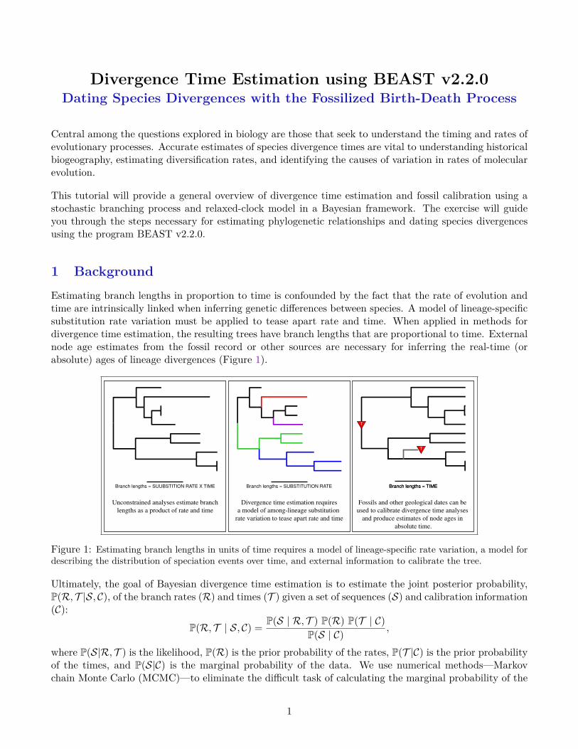
1 BackgroundEstimating branch lengths in proportion to time is confounded by the fact that the rate of evolution andtime are intrinsically linked when inferring genetic differences between species. A model of lineage-specificsubstitution rate variation must be applied to tease apart rate and time. When applied in methods fordivergence time estimation, the resulting trees have branch lengths that are proportional to time. Externalnode age estimates from the fossil record or other sources are necessary for inferring the real-time (orabsolute) ages of lineage divergences (Figure 1).
Branch lengths = SUUBSTITION RATE X TIME
Unconstrained analyses estimate branch
lengths as a product of rate and time
Branch lengths = SUBSTITUTION RATE
Divergence time estimation requires
a model of among-lineage substitution
rate variation to tease apart rate and time
Branch lengths = TIMEBranch lengths = TIME
Fossils and other geological dates can be
used to calibrate divergence time analyses
and produce estimates of node ages in
absolute time.
T
T
Figure 1: Estimating branch lengths in units of time requires a model of lineage-specific rate variation, a model fordescribing the distribution of speciation events over time, and external information to calibrate the tree.
Ultimately, the goal of Bayesian divergence time estimation is to estimate the joint posterior probability,P(R, T |S, C), of the branch rates (R) and times (T ) given a set of sequences (S) and calibration information(C):
P(R, T | S, C) = P(S | R, T ) P(R) P(T | C)P(S | C)
,
where P(S|R, T ) is the likelihood, P(R) is the prior probability of the rates, P(T |C) is the prior probabilityof the times, and P(S|C) is the marginal probability of the data. We use numerical methods—Markovchain Monte Carlo (MCMC)—to eliminate the difficult task of calculating the marginal probability of the
1
BEAST v2.0 Tutorial
data. Thus, our primary focus, aside from the tree topology, is devising probability distributions for theprior on the rates, P(R), and the prior on the times, P(T |C).
1.1 Modeling lineage-specific substitution rates
Many factors can influence the rate of substitution in a population such as mutation rate, populationsize, generation time, and selection. As a result, many models have been proposed that describe howsubstitution rate may vary across the Tree of Life.
The simplest model, the molecular clock, assumes that the rate of substitution remains constant overtime (Zuckerkandl and Pauling 1962). However, many studies have shown that molecular data (in general)violate the assumption of a molecular clock and that there exists considerable variation in the rates ofsubstitution among lineages.
Several models have been developed and implemented for inferring divergence times without assuming astrict molecular clock and are commonly applied to empirical data sets. Many of these models have beenapplied as priors using Bayesian inference methods. The implementation of dating methods in a Bayesianframework provides a flexible way to model rate variation and obtain reliable estimates of speciationtimes, provided the assumptions of the models are adequate. When coupled with numerical methods, suchas MCMC, for approximating the posterior probability distribution of parameters, Bayesian methods areextremely powerful for estimating the parameters of a statistical model and are widely used in phylogenetics.
Some models of lineage-specific rate variation:
• Global molecular clock: a constant rate of substitution over time (Zuckerkandl and Pauling 1962)• Local molecular clocks (Kishino et al. 1990; Rambaut and Bromham 1998; Yang and Yoder 2003;
Drummond and Suchard 2010)– Closely related lineages share the same rate and rates are clustered by sub-clades
• Compound Poisson process (Huelsenbeck et al. 2000)– Rate changes occur along lineages according to a point process and at rate-change events, the
new rate is a product of the old rate and a Γ-distributed multiplier.• Autocorrelated rates: substitution rates evolve gradually over the tree
– Log-normally distributed rates: the rate at a node is drawn from a log-normal distribution witha mean equal to the parent rate (Thorne et al. 1998; Kishino et al. 2001; Thorne and Kishino2002)
– Cox-Ingersoll-Ross Process: the rate of the daughter branch is determined by a non-central χ2
distribution. This process includes a parameter that determines the intensity of the force thatdrives the process to its stationary distribution (Lepage et al. 2006).
• Uncorrelated rates– The rate associated with each branch is drawn from a single underlying parametric distribution
such as an exponential or log-normal (Drummond et al. 2006; Rannala and Yang 2007; Lepageet al. 2007).
• Mixture model on branch rates– Branches are assigned to distinct rate categories according to a Dirichlet process (Heath et al.
2012).
The variety of models for relaxing the molecular clock assumption presents a challenge for investigatorsinterested in estimating divergence times. Some models assume that rates are heritable and autocorrelated
2
BEAST v2.0 Tutorial
over the tree, others model rate change as a step-wise process, and others assume that the rates oneach branch are independently drawn from a single distribution. Furthermore, studies comparing theaccuracy (using simulation) or precision of different models have produced conflicting results, some favoringuncorrelated models (Drummond et al. 2006) and others preferring autocorrelated models (Lepage et al.2007). Because of this, it is important for researchers performing these analyses to consider and testdifferent relaxed clock models (Lepage et al. 2007; Ronquist et al. 2012; Li and Drummond 2012; Baeleet al. 2013). It is also critical to take into account the scale of the question when estimating divergencetimes. For example, it might not be reasonable to assume that rates are autocorrelated if the data setincludes very distantly related taxa and low taxon sampling. In such cases, it is unlikely that any signalof autocorrelation is detectible.
1.2 Priors on node times
There are many component parts that make up a Bayesian analysis of divergence time. One that is oftenoverlooked is the prior on node times, often called a tree prior. This model describes how speciationevents are distributed over time. When this model is combined with a model for branch rate, Bayesianinference allows you to estimate relative divergence times. Furthermore, because the rate and time areconfounded in the branch-length parameter, the prior describing the branching times can have a strongeffect on divergence time estimation.
We can separate the priors on node ages into different categories:
• Phenomenological—models that make no explicit assumptions about the biological processes thatgenerated the tree. These priors are conditional on the age of the root.
– Uniform distribution: This simple model assumes that internal nodes are uniformly distributedbetween the root and tip nodes (Lepage et al. 2007; Ronquist et al. 2012).
– Dirichlet distribution: A flat Dirichlet distribution describes the placement of internal nodes onevery path between the root and tips (Kishino et al. 2001; Thorne and Kishino 2002).
• Mechanistic–models that describe the biological processes responsible for generating the pattern oflineage divergences.
– Population-level processes—models describing demographic processes (suitable for describingdifferences among individuals in the same species/population)
∗ Coalescent—These demographic models describe the time, in generations, between coales-cent events and allow for the estimation of population-level parameters (Kingman 1982c;Kingman 1982a; Kingman 1982b; Griffiths and Tavare 1994).
– Species-level processes—stochastic branching models that describe lineage diversification (suit-able for describing the timing of divergences between samples from different species)
∗ Yule (pure-birth) process: The simplest branching model assumes that, at any given pointin time, every living lineage can speciate at the same rate, λ. Because the speciation rate isconstant through time, there is an exponential waiting time between speciation events Yule(1924); Aldous (2001). The Yule model does not allow for extinction.
∗ Birth-death process: An extension of the Yule process, the birth-death model assumes thatat any point in time every lineage can undergo speciation at rate λ or go extinct at rate µ(Kendall 1948; Thompson 1975; Nee et al. 1994; Rannala and Yang 1996; Yang and Rannala1997; Popovic 2004; Aldous and Popovic 2005; Gernhard 2008). Thus, the Yule process isa special case of the birth-death process where µ = 0.
3
BEAST v2.0 Tutorial
In BEAST, the available tree priors for divergence time estimation using inter-species sequences are variantsof the birth-death prior. Extensions of the birth-death model include the calibrated Yule (Heled andDrummond 2012), the birth-death model with incomplete species sampling (Rannala and Yang 1996;Yang and Rannala 1997; Stadler 2009), and serially-sampled birth-death processes (Stadler 2010). Otherprograms also offer speciation priors as well as some alternative priors such as a uniform prior (PhyloBayes,MrBayes v3.2, DPPDiv), a Dirichlet prior (multidivtime), and a birth-death prior with species sampling(MCMCTree).
Tree priors based on the coalescent which are intended for population-level analyses virus data are alsoavailable in BEAST. The effect of different node-time priors on estimates of divergence times is not wellunderstood and appears to be dataset-dependent (Lepage et al. 2007). Accordingly, it is important toaccount for the characteristics of your data when choosing a tree prior. If you know that your sequencesare from extant species, each from different genera, then it is unlikely that a coalescent model adequatelyreflects the processes that generated those sequences. And since you do not have any samples from lineagesin the past, then you should not use the serial-sampled birth-death model. Furthermore, if you have priorknowledge that extinction has occurred, then a pure-birth (Yule) prior is not appropriate.
1.3 Calibration to absolute time
Without external information to calibrate the tree, divergence time estimation methods can only reliablyprovide estimates of relative divergence times and not absolute node ages. In the absence of adequatecalibration data, relative divergence times are suitable for analyses of rates of continuous trait evolutionor understanding relative rates of diversification. However, for some problems, such as those that seek touncover correlation between biogeographical events and lineage diversification, an absolute time scale isrequired. Calibration information can come from a variety of sources including “known” substitution rates(often secondary calibrations estimated from a previous study), dated tip sequences from serially sampleddata (typically time-stamped virus data), or geological date estimates (fossils or biogeographical data).
Age estimates from fossil organisms are the most common form of divergence time calibration information.These data are used as age constraints on their putative ancestral nodes. There are numerous difficultieswith incorporating node age estimates from fossil data including disparity in fossilization and sampling,uncertainty in dating, and correct phylogenetic placement of the fossil. Thus, it is critical that carefulattention is paid to the paleontological data included in phylogenetic divergence time analyses. With anaccurately dated and identified fossil in hand, further consideration is required to determine how to applythe node-age constraint. If the fossil is truly a descendant of the node it calibrates, then it provides areliable minimum age bound on the ancestral node time. However, maximum bounds are far more difficultto come by. Bayesian methods provide a way to account for uncertainty in fossil calibrations. Priordistributions reflecting our knowledge (or lack thereof) of the amount of elapsed time from the ancestralnode to is calibrating fossil are easily incorporated into these methods.
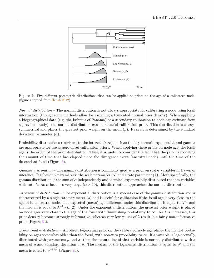
A nice review paper by Ho and Phillips (2009) outlines a number of different parametric distributionsappropriate for use as priors on calibrated nodes.
Uniform distribution – Typically, you must have both maximum and minimum age bounds when applyinga uniform calibration prior (though some methods are available for applying uniform constraints with softbounds). The minimum bound is provided by the fossil member of the clade. The maximum bound maycome from a bracketing method or other external source. This distribution places equal probability acrossall ages spanning the interval between the lower and upper bounds.
4
BEAST v2.0 Tutorial
Time
Uniform (min, max)
Exponential (λ)
Gamma (α, β)
Minimum age
Log Normal (µ, σ)
Normal (µ, σ)
(fossil)
Figure 2: Five different parametric distributions that can be applied as priors on the age of a calibrated node.(figure adapted from Heath 2012)
Normal distribution – The normal distribution is not always appropriate for calibrating a node using fossilinformation (though some methods allow for assigning a truncated normal prior density). When applyinga biogeographical date (e.g. the Isthmus of Panama) or a secondary calibration (a node age estimate froma previous study), the normal distribution can be a useful calibration prior. This distribution is alwayssymmetrical and places the greatest prior weight on the mean (µ). Its scale is determined by the standarddeviation parameter (σ).
Probability distributions restricted to the interval [0,∞), such as the log-normal, exponential, and gammaare appropriate for use as zero-offset calibration priors. When applying these priors on node age, the fossilage is the origin of the prior distribution. Thus, it is useful to consider the fact that the prior is modelingthe amount of time that has elapsed since the divergence event (ancestral node) until the time of thedescendant fossil (Figure 3).
Gamma distribution – The gamma distribution is commonly used as a prior on scalar variables in Bayesianinference. It relies on 2 parameters: the scale parameter (α) and a rate parameter (λ). More specifically, thegamma distribution is the sum of α independently and identical exponentially distributed random variableswith rate λ. As α becomes very large (α > 10), this distribution approaches the normal distribution.
Exponential distribution – The exponential distribution is a special case of the gamma distribution and ischaracterized by a single rate parameter (λ) and is useful for calibration if the fossil age is very close to theage of its ancestral node. The expected (mean) age difference under this distribution is equal to λ−1 andthe median is equal to λ−1 ∗ ln(2). Under the exponential distribution, the greatest prior weight is placedon node ages very close to the age of the fossil with diminishing probability to ∞. As λ is increased, thisprior density becomes strongly informative, whereas very low values of λ result in a fairly non-informativeprior (Figure 3a).
Log-normal distribution – An offset, log-normal prior on the calibrated node age places the highest proba-bility on ages somewhat older than the fossil, with non-zero probability to ∞. If a variable is log-normallydistributed with parameters µ and σ, then the natural log of that variable is normally distributed with amean of µ and standard deviation of σ. The median of the lognormal distribution is equal to eµ and themean is equal to eµ+ σ2
2 (Figure 3b).
5
BEAST v2.0 Tutorial
λ = 5-1
λ = 20-1
λ = 60-1
De
nsity
Node age - Fossil age0 80604020 100
60
80
100
120
140
a) Exponential prior density
Exp
ecte
d n
od
e a
ge
Min age
(fossil)E
xp
ecte
d n
od
e a
ge
Min age
(fossil)
De
nsity
Node age - Fossil age0 252015105 30
30
35
40
45
b) Lognormal prior density
Figure 3: Two common prior densities for calibrating node ages. a) The exponential distribution with three differentvalues for the rate parameter, λ. As the value of the λ rate parameter is decreased, the prior becomes less informative(the blue line is the least informative prior, λ = 60−1). The inset shows an example of the three different priorsand their expected values placed on the same node with a minimum age bound of 60. b) The lognormal distributionwith 3 different values for the shape parameter, σ. For this distribution, even though µ is equal to 2.0 for all three,expected value (mean) is dependent on the value of σ. The inset shows an example of the three different priors andtheir expected values placed on the same node with a minimum age bound of 30.
1.4 Integrating Fossil Occurrence Times in the Speciation Model
Calibrating Bayesian divergence-time estimates using parametric densities (as described in the previoussection: Sec. 1.3) is ultimately a difficult and unsatisfactory approach, particularly if the calibration infor-mation comes from fossil occurrence times. The calibration densities are typically applied in a multiplicativemanner such that the prior probability of a calibrated node age is the product o the probability comingfrom the tree-wide speciation model and the probability under the calibration density (Heled and Drum-mond 2012; Warnock et al. 2012; Warnock et al. 2015). This approach leads to an incoherence and inducesa prior that is inconsistent with the described calibration density. This statistical incoherence has beencorrected by conditional tree prior models (Yang and Rannala 2006; Heled and Drummond 2012; Heledand Drummond 2013). These conditional approaches are an important contribution to the field, particu-larly when non-fossil data are used to calibrate an analysis. However, when using fossil information, it ismore appropriate to account for the fact that the fossils are part of the same diversification process (i.e.,birth-death model) that generated the extant species.
1.4.1 The Fossilized Birth-Death Process
The exercise outlined in this tutorial demonstrates how to calibrate species divergence using the fossilizedbirth-death (FBD) model described in Stadler (2010) and Heath et al. (2014). This model simply treats thefossil observations as part of the prior on node times, such as the birth-death models outlined in Section1.2 of this document. The fossilized birth-death process provides a model for the distribution of speciationtimes, tree topology, and distribution of lineage samples before the present (i.e., non-contemporaneoussamples like fossils or viruses). Importantly, this model can be used with or without character data for thehistorical samples. Thus, it provides a reasonable prior distribution for analyses combining morphologicalor DNA data for both extant and fossil taxa—i.e, the so-called ‘total-evidence’ approaches described byRonquist et al. (2012) (also see Pyron 2011). When matrices of discrete morphological characters for both
6
BEAST v2.0 Tutorial
living and fossil species are unavailable, the fossilized birth-death model imposes a time structure on thetree by marginalizing over all possible attachment points for the fossils on the extant tree (Heath et al.2014), therefore, some prior knowledge of phylogenetic relationships is important, much like for calibration-density approaches.
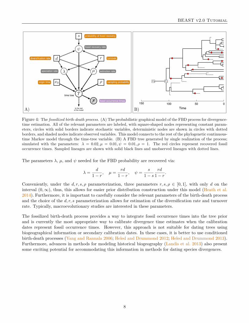
The FBD model describes the probability of the tree and fossils conditional on the birth-death parameters:f [T | λ, µ, ρ, ψ, xc], where T denotes the tree topology, divergence times, fossil occurrence times, and thetimes at which the fossils attach to the tree. The parameters of the model are:
λ speciation rateµ extinction rateρ probability of sampling extant speciesψ fossil recovery ratexc the starting time of the process, either x0 or x1
Figure 4A shows the probabilistic graphical model of the FBD process. Additionally, an example FBD treeis shown in Figure 4B, where the diversification process originates at time x0, giving rise to n = 20 speciesin the present. All of the lineages represented in Figure 4B (both solid and dotted lines) show the completetree. This is the tree of all extant and extinct lineages generated by the process. The complete tree isdistinct from the reconstructed tree which is the tree representing only the sampled extant lineages. Fossilobservations (red circles in Figure 4B) are recovered over the process along the lineages of the completetree. If a lineage does not have any descendants sampled in the present, it is lost and cannot be observed,these are the dotted lines in Figure 4B. The probability must be conditioned on the starting time of theprocess xc. This can be one of two different nodes in the tree, either the origin time x0 or the root agex1 (Figure 4B). The origin (x0) of a birth death process is the starting time of the stem lineage, thus thisconditions on a single lineage giving rise to the tree. Alternatively, a birth-death process can be conditionedon the age of the root (x1), which is the time of the most-recent-common ancestor (MRCA) of the sampledlineages. Here, the model assumes that the branching process starts with two lineages, each of which hasthe same starting time.
An important characteristic of the FBD model is that it accounts for the probability of sampled ancestor-descendant pairs (Foote 1996). Given that fossils are sampled from lineages in the diversification process,the probability of sampling fossils that are ancestors to taxa sampled at a later date is correlated with theturnover rate (r = µ/λ) and the fossil recovery rate (ψ). This feature is important, particularly for datasetswith many sampled fossils. In the example (Figure 4B), several of the fossils have sampled descendants.These fossils have solid black lines leading to the present.
Recently, Gavryushkina et al. (2014) extended the fossilized birth-death model to allow more flexibilityin the assignment of fossils to clades and conditioning parameters and implemented this version in theBEAST2 package called SA (“Sampled Ancestors”, by Alexandra Gavryushkina). Notably, this imple-mentation also allows you to use the FBD model as a tree prior for datasets combining molecular data fromextant taxa with morphological data for both fossil and extant species. In this implementation of the FBDmodel, instead of the parameters λ, µ, and ψ, the following parameters are used in MCMC optimization:
d = λ− µ Net diversification rater = µ/λ Turnover
s = ψ/(µ+ ψ) Probability of fossil observation prior to species extinction
7
BEAST v2.0 Tutorial
A) B)150 100 50 0
Time
Figure 4: The fossilized birth-death process. (A) The probabilistic graphical model of the FBD process for divergence-time estimation. All of the relevant parameters are labeled, with square-shaped nodes representing constant param-eters, circles with solid borders indicate stochastic variables, deterministic nodes are shown in circles with dottedborders, and shaded nodes indicate observed variables. This model connects to the rest of the phylogenetic continuous-time Markov model through the time-tree variable. (B) A FBD tree generated by single realization of the process;simulated with the parameters: λ = 0.02, µ = 0.01, ψ = 0.01, ρ = 1. The red circles represent recovered fossiloccurrence times. Sampled lineages are shown with solid black lines and unobserved lineages with dotted lines.
The parameters λ, µ, and ψ needed for the FBD probability are recovered via:
λ = d
1 − r, µ = rd
1 − r, ψ = s
1 − s
rd
1 − r.
Conveniently, under the d, r, s, ρ parameterization, three parameters r, s, ρ ∈ [0, 1], with only d on theinterval (0,∞), thus, this allows for easier prior distribution construction under this model (Heath et al.2014). Furthermore, it is important to carefully consider the relevant parameters of the birth-death processand the choice of the d, r, s parameterization allows for estimation of the diversification rate and turnoverrate. Typically, macroevolutionary studies are interested in these parameters.
The fossilized birth-death process provides a way to integrate fossil occurrence times into the tree priorand is currently the most appropriate way to calibrate divergence time estimates when the calibrationdates represent fossil occurrence times. However, this approach is not suitable for dating trees usingbiogeographical information or secondary calibration dates. In these cases, it is better to use conditionedbirth-death processes (Yang and Rannala 2006; Heled and Drummond 2012; Heled and Drummond 2013).Furthermore, advances in methods for modeling historical biogeography (Landis et al. 2013) also presentsome exciting potential for accommodating this information in methods for dating species divergences.
8
BEAST v2.0 Tutorial
2 Programs used in this ExerciseBEAST – Bayesian Evolutionary Analysis Sampling TreesBEAST is a free software package for Bayesian evolutionary analysis of molecular sequences using MCMCand strictly oriented toward inference using rooted, time-measured phylogenetic trees (Drummond et al.2006; Drummond and Rambaut 2007; Bouckaert et al. 2014). The development and maintenance of BEASTis a large, collaborative effort and the program includes a wide array of different types of analyses:
• Phylogenetic tree inference under different models for substitution rate variation– Constant rate molecular clock (Zuckerkandl and Pauling 1962)– Uncorrelated relaxed clocks (Drummond et al. 2006)– Random local molecular clocks (Drummond and Suchard 2010)
• Estimates of species divergence dates and fossil calibration under a wide range of branch-time modelsand calibration methods
• Analysis of non-contemporaneous sequences• Heterogenous substitution models across data partitions• Population genetic analyses
– Estimation of demographic parameters (population sizes, growth/decline, migration)– Bayesian skyline plots– Phylogeography (Lemey et al. 2009)
• Gene-tree/species-tree inference (∗BEAST; Heled and Drummond 2010)• and more...
BEAST is written in java and its appearance and functionality are consistent across platforms. Inferenceusing MCMC is done using the BEAST program, however, there are several utility applications that assistin the preparation of input files and summarize output (BEAUti, LogCombiner, and TreeAnnotator areall part of the BEAST software bundle).
There are currently two available versions of the BEAST package:BEAST v1.8 http://beast.bio.ed.ac.uk (BEAST 1)BEAST v2.1.2 http://www.beast2.org/ (BEAST 2).
BEAST 2 is a complete re-write of BEAST 1, with different design choices (Bouckaert et al. 2014). TheBEAST 2 package allows for implementation and distribution of new models and methods through add-ons(also called “plugins”). Add-ons include SNAPP (phylogenetic analysis using SNP and AFLP data) andBDSSM (a birth-death skyline model for serially-sampled data), as well as several others that are availableor in development. It is important to note, however, that the set of analyses and models available in theBEAST 2 package do not completely overlap with the set of analyses with BEAST 1 (though this shouldnot be the case in the near future). I strongly encourage you to learn more about BEAST and the BEASTv2 software by reading the book provided online by the developers: Bayesian Evolutionary Analysis withBEAST 2 (Drummond and Bouckaert 2014).
BEAUti – Bayesian Evolutionary Analysis UtilityBEAUti is a utility program with a graphical user interface for creating BEAST and *BEAST input fileswhich must be written in the eXtensible Markup Language (XML). This application provides a clear wayto specify priors, partition data, calibrate internal nodes, etc.
LogCombiner – When multiple (identical) analyses are run using BEAST (or MrBayes), LogCombinercan be used to combine the parameter log files or tree files into a single file that can then be summarizedusing Tracer (log files) or TreeAnnotator (tree files). However, it is important to ensure that all analysesreached convergence and sampled the same stationary distribution before combining the parameter files.
TreeAnnotator – TreeAnnotator is used to summarize the posterior sample of trees to produce a maxi-mum clade credibility tree and summarize the posterior estimates of other parameters that can be easilyvisualized on the tree (e.g. node height). This program is also useful for comparing a specific tree topologyand branching times to the set of trees sampled in the MCMC analysis.
Tracer – Tracer is used for assessing and summarizing the posterior estimates of the various parameterssampled by the Markov Chain. This program can be used for visual inspection and assessment of conver-gence and it also calculates 95% credible intervals (which approximate the 95% highest posterior densityintervals) and effective sample sizes (ESS) of parameters (http://tree.bio.ed.ac.uk/software/tracer).
FigTree – FigTree is an excellent program for viewing trees and producing publication-quality fig-ures. It can interpret the node-annotations created on the summary trees by TreeAnnotator, allow-ing the user to display node-based statistics (e.g. posterior probabilities) in a visually appealing way(http://tree.bio.ed.ac.uk/software/figtree).
R – Viewing and Plotting TreesFor this exercise we will use some R packages to visualize the summary tree with a geological timescale. Ifyou do not already have R installed, please download the current version: http://www.r-project.org
strap – Viewing dated phylogenies with an arbitrary time-scale removes the context of geological timeand the fossil record from the analysis. The package strap in R provides a set of functions to plot treesand stratigraphic information against geologic time, with scales provided by different sources includingthe International Commission on Stratigraphy (Bell and Lloyd 2014). A detailed tutorial for using thefunctions in strap is available here: http://datadryad.org/resource/doi:10.5061/dryad.4k078. To installstrap, execute the following command in R:
phytools – In R, there are many packages available for performing phylogenetic comparative methods,among them phytools is one of the richest, providing functions for a wide range of different analyses andfor visualizing evolutionary processes in the context of phylogenetic relationships (Revell 2012). To installphytools in R, execute the following command:
phyloch – The trees sampled by the MCMC in BEAST contain valuable information about the sampleddivergence times and branch rates. Additionally, the summary trees produced by the BEAST accessoryprogram TreeAnnotator have information about the 95% credible intervals for the ages and rates. Thepackage phyloch provides functions for reading in data files written by BEAST and its accessory programs(Heibl 2008). This package, however, is not available for download from CRAN. Instead, it is hosted on
The eXtensible Markup Language (XML) is a general-purpose markup language, which allows for thecombination of text and additional information. In BEAST, the use of the XML makes analysis specificationvery flexible and readable by both the program and people. The XML file specifies sequences, nodecalibrations, models, priors, output file names, etc. BEAUti is a useful tool for creating an XML filefor many BEAST analyses. However, typically, dataset-specific issues can arise and some understandingof the BEAST-specific XML format is essential for troubleshooting. Additionally, there are a numberof interesting models and analyses available in BEAST that cannot be specified using the BEAUti utilityprogram. Refer to the BEAST web page (http://beast.bio.ed.ac.uk/XML_format) for detailed informationabout the BEAST XML format. Box 1 shows an example of BEAST XML syntax for specifying a birth-death prior on node times.
<!- An exponential prior distribution on the gamma shape parameter of the irbp gene -><prior id =" GammaShapePrior .s:irbp" name =" distribution " x=" @gammaShape .s:irbp">
<Exponential id =" Exponential .01" name =" distr "><parameter id =" RealParameter .01" lower ="0.0" name =" mean" upper ="0.0" >1.0 </
parameter ></ Exponential >
</prior >
Box 1: BEAST 2 XML specification of an exponential prior density on the shape of a gamma distribution.
4 Practical: Divergence Time EstimationThis tutorial will walk you through an analysis of the divergence times of the bears. The occurrence timesof 14 fossil species are integrated into the tree prior to impose a time structure on the tree and calibrate theanalysis to absolute time. Additionally, an uncorrelated, lognormal relaxed clock model is used to describethe branch-specific substitution rates.
The analysis in this tutorial includes data from several different sources. We have molecular sequencedata for eight extant species, which represent all of the living bear taxa. The sequence data includeinterphotoreceptor retinoid-binding protein (irbp) sequences (in the file bears_irbp_fossils.nex) and1000 bps of the mitochondrial gene cytochrome b (in the file bears_cytb_fossils.nex). If you openeither of these files in your text editor or alignment viewer, you will notice that there are 22 taxa listed ineach one, with most of these taxa associated with sequences that are entirely made up of missing data (i.e.,?????). The NEXUS files contain the names of 14 fossil species, that we will include in our analysis ascalibration information for the fossilized birth-death process. Further, we must provide an occurrence timefor each taxon sampled from the fossil record. For the fossil species, this information is obtained from theliterature or fossil databases like the Fossilworks PaleoDB or the Fossil Calibration Database, or from yourown paleontological expertise. The 14 fossil species used in this analysis are listed in Table 1 along withthe age range for the specimen and relevant citation. For this exercise, we will fix the ages to a value withinthe age range provided in Table 1. In BEAST2, it is possible to use MCMC to sample the occurrencetime for a fossil conditional on a prior distribution. However, the options to do this are not currentlyavailable in BEAUti, and will not be covered by this tutorial. The age of each taxon is encoded in thetaxon name following the last ‘_’ character. For example, the fossil panda Kretzoiarctos beatrix has an ageof approximately 11.7 Mya, thus, the taxon name in the alignment files is: Kretzoiarctos_beatrix_11.7.Similarly, since the polar bear, Ursus maritimus, represents an extant species, its occurrence time is 0.0Mya, which makes its taxon name: Ursus_maritimus_0. By including the tip ages in the taxon names,we can easily import these values into BEAUti while setting up the XML file. This is simply easier thanentering them in by hand (which is also possible).
The final source of data required for our analysis is some information about the phylogenetic placementof the fossils. This prior knowledge can come from previous studies of morphological data and taxonomy.Ideally, we would know exactly where in the phylogeny each fossil belongs. However, this is uncommonfor most groups in the fossil record. Often, we can place a fossil with reasonable resolution by assigning itto some total group. For example, if a fossil specimen has all of the identifying characters of a bear in thesubfamily Ursinae, then, we can create a monophyletic group of all known Ursinae species and our fossil.Here, we would be assigning the fossil to the total group Ursinae, meaning that the fossil can be a crownor stem fossil of this group. For some fossils, we may have very little data to inform their placement inthe tree and perhaps we may only know that it falls somewhere within our group of interest. In this case,we can account for our uncertainty in the relationship of the fossil and all other taxa and allow MCMC to
Table 1: Fossil species used for calibrating divergence times under the FBD model. Modified from TableS.3 in the supplemental appendix of Heath et al. (2014).
Fossil species Age range (My) CitationParictis montanus 33.9–37.2 Clark and Guensburg 1972; Krause et al. 2008Zaragocyon daamsi 20–22.8 Ginsburg and Morales 1995; Abella et al. 2012Ballusia elmensis 13.7–16 Ginsburg and Morales 1998; Abella et al. 2012Ursavus primaevus 13.65–15.97 Andrews and Tobien 1977; Abella et al. 2012Ursavus brevihinus 15.97–16.9 Heizmann et al. 1980; Abella et al. 2012Indarctos vireti 7.75–8.7 Montoya et al. 2001; Abella et al. 2012Indarctos arctoides 8.7–9.7 Geraads et al. 2005; Abella et al. 2012Indarctos punjabiensis 4.9–9.7 Baryshnikov 2002; Abella et al. 2012Ailurarctos lufengensis 5.8–8.2 Jin et al. 2007; Abella et al. 2012Agriarctos spp. 4.9–7.75 Abella et al. 2011; Abella et al. 2012Kretzoiarctos beatrix 11.2–11.8 Abella et al. 2011; Abella et al. 2012Arctodus simus 0.012–2.588 Churcher et al. 1993; Krause et al. 2008Ursus abstrusus 1.8–5.3 Bjork 1970; Krause et al. 2008Ursus spelaeus 0.027–0.25 Loreille et al. 2001; Krause et al. 2008
sample all possible places where the fossil can attach in the tree. For the bear species in our analysis, wehave some prior knowledge about their relationships, represented as an unresolved phylogeny in Figure 5.We will input this information when constructing our analysis file in BEAUti.
Agriarctos spp X
Ailurarctos lufengensis X
Ailuropoda melanoleuca
Arctodus simus X
Ballusia elmensis X
Helarctos malayanus
Indarctos arctoides X
Indarctos punjabiensis X
Indarctos vireti X
Kretzoiarctos beatrix X
Melursus ursinus
Parictis montanus X
Tremarctos ornatus
Ursavus brevihinus X
Ursavus primaevus X
Ursus abstrusus X
Ursus americanus
Ursus arctos
Ursus maritimus
Ursus spelaeus X
Ursus thibetanus
Zaragocyon daamsi X
Ste
m
Be
ars
Cro
wn
Be
ars
Pandas
Tremarctinae
Brown Bears
Ursinae
Origin
Root(Total Group)
Crown
Figure 5: The phylogenetic relationships of crown and stem bears based on taxonomy and morphological data. Theresolution of monophyletic clades is based on well-supported previous analyses. Monophyletic clades are indicatedwith labeled circles. In addition to the root node (R), there are 5 nodes defining clades containing both fossil andextant species. The origin of the tree is indicated with a red square. The time of this node represents the start ofthe diversification process that generated these linages. The extant lineages are shown with heavy, solid lines andthe fossil lineages are dotted lines.
4.2 Creating the Analysis File with BEAUti
Creating a properly-formatted BEAST XML file from scratch is not a simple task. However, BEAUtiprovides a simple way to navigate the various elements specific to the BEAST XML format.
13
BEAST v2.0 Tutorial
Begin by executing the BEAUti program
Be sure that this is the version that came from the BEAST 2 download from: http://beast2.org. For MacOSX and Windows, you can do this by double clicking on the application. For Unix systems (includingMac OSX), it is convenient to add the entire BEAST/bin directory to your path.
4.2.1 Install BEAST 2 Plug-Ins
Next, we have to install the BEAST 2 packages (also called “plug-ins” or “add-ons”) that are needed forthis analysis. The package that we will use is called SA.
Open the BEAST 2 Package Manager by navigating to File→Manage Packages in the menu.[Figure 6]
In the package manager, you can install all of the available plug-ins for BEAST 2. These include anumber of packages for analyses such as species delimitation (DISSECT, STACEY), population dynamics(MASTER), the phylodynamics of infectious disease (BDSKY, phylodynamics), etc.
Install the SA package by selecting it and clicking the Install/Upgrade button. [Figure 6]
Figure 6: The BEAST2 Package Manager.
It is important to note that you only need to install a BEAST 2 package once, thus if you close BEAUti,you don’t have to load SA the next time you open the program. However, it is worth checking the packagemanager for updates to plug-ins, particularly if you update your version of BEAST 2.
Close the BEAST 2 Package Manager and restart BEAUti to fully load the SA package.
4.2.2 Import Alignments
Navigate to the Partitions window (you should already be here).
Next we will load the alignment files for each of our genes. Note that separate loci can be imported asseparate files or in a single NEXUS file with partitions defined using the ASSUMPTIONS command.
Using the menu commands File→Import Alignment, import the data files:bears_irbp_fossils.nex and bears_cytb_fossils.nex
Now that the data are loaded into BEAUti, we can unlink the site models, link the clock models, link thetrees and rename these variables.
Highlight both partitions (using shift+click) and click on Unlink Site Models to assume differentmodels of sequence evolution for each gene (the partitions are typically already unlinked by default).
Now click the Link Clock Models button so that the two genes have the same relative rates ofsubstitution among branches.
Finally click Link Trees to ensure that both partitions share the same tree topology and branchingtimes.
It is convenient to rename some of the variables in the Partitions window. By doing this, the parametersassociated with each partition that are written to file are a bit more intuitively labeled.
Double click on the site model for the cytochrome b gene, it is currently called bears_cytb_fossils.Rename this: cytb. (Note that you may have to hit the return or enter key after typing in the newlabel for the new name to be retained.)
Do the same for the site model for the other gene, calling it irbp.
Rename the clock model bearsClock.
Rename the tree bearsTree. [Figure 7]
Figure 7 shows how the final Partitions window should look.
15
BEAST v2.0 Tutorial
Figure 7: The Partitions window after unlinking the site models, linking the clock models, linking the trees, andrenaming the XML variables.
4.2.3 Set Tip Dates
Navigate to the Tip Dates panel.
We must indicate that we have sequentially sampled sequences. When performing an analysis withoutdated tips or any fossil information, you can skip this window, and BEAST will assume that all of yoursamples are contemporaneous.
Toggle on the Use tip dates option.
The next step involves specifying how the dates are oriented on the tree and the units they are in. We willindicate that the dates are in years, even though they are in fact in units of millions of years. This isbecause the units themselves are arbitrary and this scale difference will not matter. Additionally, we willtell BEAUti that the zero time of our tree is the present and the ages we are providing are the number ofyears Before the present.
Change: Dates specified as: year Before the present [Figure 8]
For some types of analyses, such as serially sampled viruses, the dates given are relative to some time inthe past, thus this option is available as well.
Figure 8: Specifying the units and reference point of the fossil dates.
When inputing the dates for each tip species, one option is to enter each one by hand. This may be quiteonerous if you have many fossils or many sequences sampled back in time. Conveniently, these dates canbe included in the taxon names so that BEAUti can easily extract them for us using the Guess option.
Click on the Guess button.
This will open a window where you can specify the pattern in the taxon names from which the tip agescan be extracted. Obviously, it’s better to make this a fairly simple code that doesn’t require multiple
16
BEAST v2.0 Tutorial
iterations of searches. Moreover, if this is straightforward, then you will be able to easily eliminate thesedates when creating figures from your final summary tree.
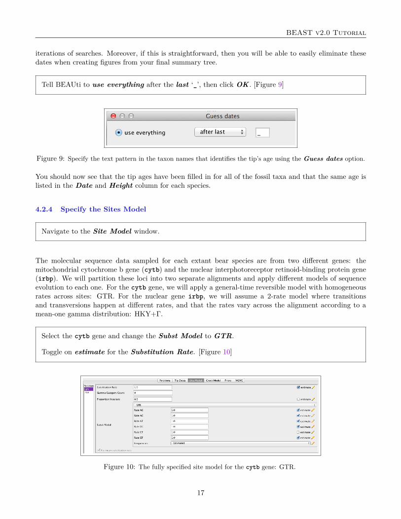
Tell BEAUti to use everything after the last ‘_’, then click OK . [Figure 9]
Figure 9: Specify the text pattern in the taxon names that identifies the tip’s age using the Guess dates option.
You should now see that the tip ages have been filled in for all of the fossil taxa and that the same age islisted in the Date and Height column for each species.
4.2.4 Specify the Sites Model
Navigate to the Site Model window.
The molecular sequence data sampled for each extant bear species are from two different genes: themitochondrial cytochrome b gene (cytb) and the nuclear interphotoreceptor retinoid-binding protein gene(irbp). We will partition these loci into two separate alignments and apply different models of sequenceevolution to each one. For the cytb gene, we will apply a general-time reversible model with homogeneousrates across sites: GTR. For the nuclear gene irbp, we will assume a 2-rate model where transitionsand transversions happen at different rates, and that the rates vary across the alignment according to amean-one gamma distribution: HKY+Γ.
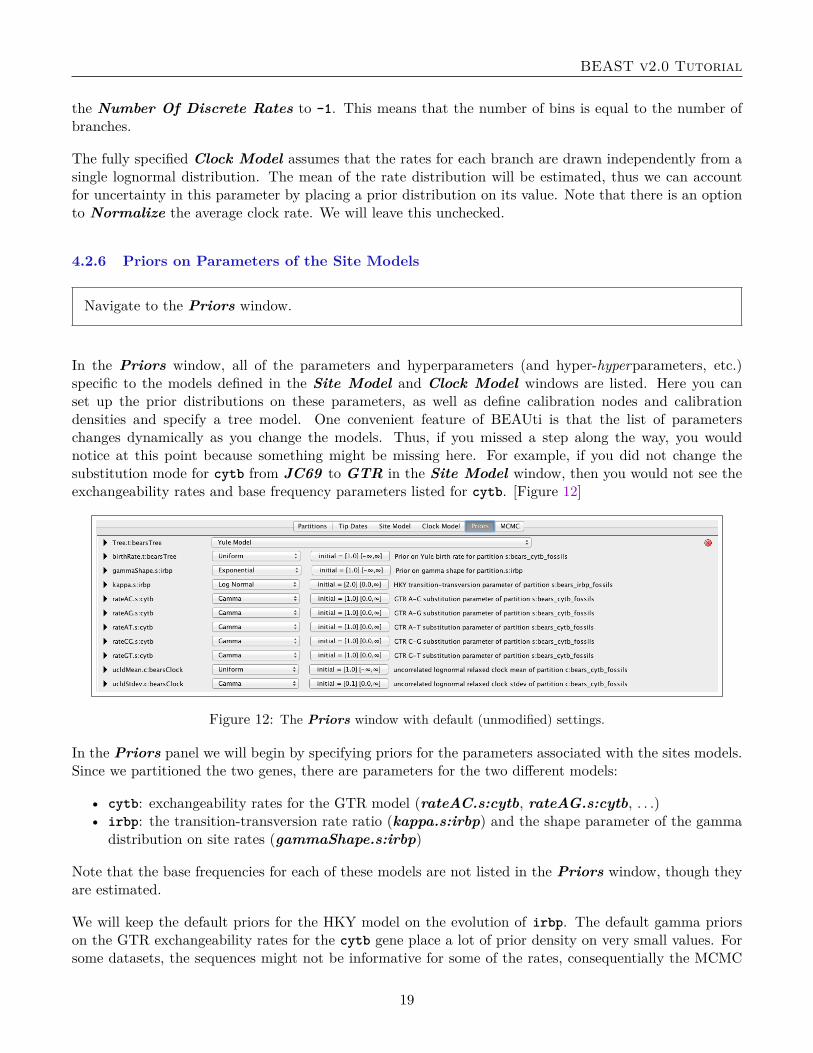
Select the cytb gene and change the Subst Model to GTR.
Toggle on estimate for the Substitution Rate. [Figure 10]
Figure 10: The fully specified site model for the cytb gene: GTR.
17
BEAST v2.0 Tutorial
By changing the substitution model, we have now introduced additional parameters for the GTR exchange-ability rates. We will construct priors for these parameters later on.
Select the irbp gene and change the Subst Model to HKY .
To indicate gamma-distributed rates, set the Gamma Category Count to 4.
Then switch the Shape parameter to estimate.
Toggle on estimate for the Substitution Rate. [Figure 11]
Figure 11: The fully specified site model for the irbp gene: HKY+Γ.
Now both models are fully specified for the unlinked genes. Note that Fix mean substitution rate isalways specified and we also have indicated that we wish to estimate the Substitution Rate for eachgene. This means that we are estimating the relative substitution rates for our two loci.
4.2.5 The Clock Model
Navigate to the Clock Model window.
Here, we can specify the model of lineage-specific substitution rate variation. The default model in BEAUtiis the Strict Clock with a fixed substitution rate equal to 1. Three models for relaxing the assumptionof a constant substitution rate can be specified in BEAUti as well. The Relaxed Clock Log Normaloption assumes that the substitution rates associated with each branch are independently drawn from asingle, discretized lognormal distribution (Drummond et al. 2006). Under the Relaxed Clock Exponentialmodel, the rates associated with each branch are exponentially distributed (Drummond et al. 2006). TheRandom Local Clock uses Bayesian stochastic search variable selection to average over random localmolecular clocks (Drummond and Suchard 2010). For this analysis we will use the uncorrelated, lognormalmodel of branch-rate variation.
Change the clock model to Relaxed Clock Log Normal.
The uncorrelated relaxed clock models in BEAST2 are discretized for computational feasibility. This meansthat for any given parameters of the lognormal distribution, the probability density is discretized into somenumber of discrete rate bins. Each branch is then assigned to one of these bins. By default, BEAUti sets
18
BEAST v2.0 Tutorial
the Number Of Discrete Rates to -1. This means that the number of bins is equal to the number ofbranches.
The fully specified Clock Model assumes that the rates for each branch are drawn independently from asingle lognormal distribution. The mean of the rate distribution will be estimated, thus we can accountfor uncertainty in this parameter by placing a prior distribution on its value. Note that there is an optionto Normalize the average clock rate. We will leave this unchecked.
4.2.6 Priors on Parameters of the Site Models
Navigate to the Priors window.
In the Priors window, all of the parameters and hyperparameters (and hyper-hyperparameters, etc.)specific to the models defined in the Site Model and Clock Model windows are listed. Here you canset up the prior distributions on these parameters, as well as define calibration nodes and calibrationdensities and specify a tree model. One convenient feature of BEAUti is that the list of parameterschanges dynamically as you change the models. Thus, if you missed a step along the way, you wouldnotice at this point because something might be missing here. For example, if you did not change thesubstitution mode for cytb from JC69 to GTR in the Site Model window, then you would not see theexchangeability rates and base frequency parameters listed for cytb. [Figure 12]
Figure 12: The Priors window with default (unmodified) settings.
In the Priors panel we will begin by specifying priors for the parameters associated with the sites models.Since we partitioned the two genes, there are parameters for the two different models:
• cytb: exchangeability rates for the GTR model (rateAC.s:cytb, rateAG.s:cytb, . . .)• irbp: the transition-transversion rate ratio (kappa.s:irbp) and the shape parameter of the gamma
distribution on site rates (gammaShape.s:irbp)
Note that the base frequencies for each of these models are not listed in the Priors window, though theyare estimated.
We will keep the default priors for the HKY model on the evolution of irbp. The default gamma priorson the GTR exchangeability rates for the cytb gene place a lot of prior density on very small values. Forsome datasets, the sequences might not be informative for some of the rates, consequentially the MCMC
19
BEAST v2.0 Tutorial
may propose values very close to zero and this can induce long mixing times. Because of this problem, wewill alter the gamma priors on the exchangeability rates. For each one, we will keep the expected valuesas in the default priors. The default priors assume that transitions (A↔G or C↔T) have an expected rateof 1.0. Remember that we fixed the parameter rateCT to equal 1.0 in the Site Model window, thusthis parameter isn’t in the Priors window. For all other rates, transversions, the expected value of thepriors is lower: 0.5. In BEAST, the gamma distribution is parameterized by a shape parameter (Alpha)and a scale parameter (Beta). Under this parameterization, expected value for any gamma distributionis: E(x) = αβ. To reduce the prior density on very low values, we can increase the shape parameter andthen we have to adjust the scale parameter accordingly.
Begin by changing the gamma prior on the transition rate rateAG.s:cytb. Clicking on the ▶ next tothis parameter name to reveal the prior options. Change the parameters: Alpha = 2 and Beta = 0.5.[Figure 13, bottom]
Then change all of the other rates: rateAC.s, rateAT.s, rateCG.s, rateGT.s. Fore each of these,change the parameters to: Alpha = 2 and Beta = 0.25. [Figure 13, top]
Figure 13: Gamma prior distributions on two of the five relative rates of the GTR model.
4.2.7 Priors for the Clock Model
Since we are assuming that the branch rates are drawn from a lognormal distribution, this induces twohyperparameters: the mean and standard deviation (ucldMean.c and ucldStdev.c respectively). Bydefault, the prior distribution on the ucldMean.c parameter is an improper, uniform distribution on theinterval (0,∞). Note that this type of prior is called improper because the prior density of a uniformdistribution with infinite bounds does not integrate to 1. Although improper priors can sometimes lead toproper posterior distributions, they may also have undesired effects and cause problems with mixing andconvergence.
Reveal the options for the prior on ucldMean.c by clicking on the ▶. Change the prior density to anExponential with a mean of 10.0. [Figure 14]
20
BEAST v2.0 Tutorial
Figure 14: The exponential prior distribution on the mean of the log normal relaxed clock model.
The other parameter of our relaxed-clock model is, by default assigned a gamma prior distribution. How-ever, we have a strong prior belief that the variation in substitution rates among branches is low, sincesome previous studies have indicated that the rates of molecular evolution in bears is somewhat clock-like(Krause et al. 2008). Thus, we will assume an exponential prior distribution with 95% of the probabilitydensity on values less than 1 for the ucldStdev.c parameter.
Reveal the options for the prior on ucldStdev.c by clicking on the ▶. Change the prior density to anExponential with a mean of 0.3337. [Figure 15]
Figure 15: The exponential prior distribution on the standard deviation of the log normal relaxed clock model.
4.2.8 The Tree Prior
Next we will specify the prior distribution on the tree topology and branching times. You should noticean error notification (a red circle with an “X” in it) in the Priors panel to the left of Tree.t:bearsTree(Figure 12). If you mouse over this notification, you will se a message telling you that the default YuleModel is not appropriate for non-contemporaneous tips and that you must choose a different tree prior.Thus, here is where we specify the fossilized birth-death process.
Change the tree model for Tree.t:bearsTree to Fossilized Birth Death Model. [Figure 16]
Reveal the options for the prior on Tree.t by clicking on the ▶.
Origin Time — In Section 1.4.1, the parameters of the FBD model are given. Remember that this model,like any branching process (i.e., constant rate birth-death, Yule) can be conditioned on either the origintime or the root age. Depending on the available prior information or the type of data available, it makes
21
BEAST v2.0 Tutorial
Figure 16: The tree priors available for specification in BEAUti.
sense to condition on one or the other (but not both, obviously). If you know that all of the fossils inyour dataset are crown fossils—descendants of the MRCA of all the extant taxa—and you have some priorknowledge of the age of the clade, then it is reasonable to condition the FBD on the root. Alternatively,if the fossils in your analysis are stem fossils, or can only reliably be assigned to your total group, then itis appropriate to condition on the origin age.
For this analysis, we have several bear fossils that are considered stem fossils, thus we will condition onthe origin age. Previous studies (dos Reis et al. 2012) estimated an age of approximately 45.5 My for theMRCA of seals and bears. We will use this time as a starting value for the origin.
Set the starting value of the Origin to 45.5 and specify that this parameter will be estimated bychecking the estimate box. (You may have to expand the width of the BEAUti window to see thecheck-boxes for these parameters.) [Figure 17]
Figure 17: The initial values and conditions for the fossilized birth-death process (Stadler 2010; Heath et al. 2014;Gavryushkina et al. 2014)
Since we are estimating the origin parameter, we must assign a prior distribution to it (unless we wishto keep the default Uniform(0,∞) prior). We will assume that the origin time is drawn from a lognormaldistribution with an expected value (mean) equal to 45.5 My and a standard deviation of 1.0.
Reveal the options for the prior on originFBD.t by clicking on the ▶.
Change the prior distribution to Log Normal.
Check the box marked Mean In Real Space and set the mean M equal to 8.5 and the standarddeviation S to 1.0.
22
BEAST v2.0 Tutorial
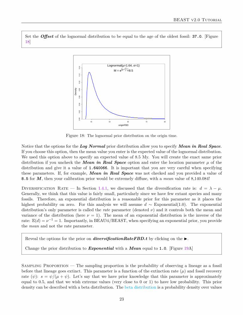
Set the Offset of the lognormal distribution to be equal to the age of the oldest fossil: 37.0. [Figure18]
40 50 60 70 80
0.00
0.02
0.04
0.06
0.08
0.10
0.12
0.14
originFBD
Den
sity
Lognormal(µ=1.64, σ=1)
M = e(µ−σ2
2 )=8.5
Figure 18: The lognormal prior distribution on the origin time.
Notice that the options for the Log Normal prior distribution allow you to specify Mean in Real Space.If you choose this option, then the mean value you enter is the expected value of the lognormal distribution.We used this option above to specify an expected value of 8.5 My. You will create the exact same priordistribution if you uncheck the Mean in Real Space option and enter the location parameter µ of thedistribution and give it a value of 1.640066. It is important that you are very careful when specifyingthese parameters. If, for example, Mean in Real Space was not checked and you provided a value of8.5 for M , then your calibration prior would be extremely diffuse, with a mean value of 8,140.084!
Diversification Rate — In Section 1.4.1, we discussed that the diversification rate is: d = λ − µ.Generally, we think that this value is fairly small, particularly since we have few extant species and manyfossils. Therefore, an exponential distribution is a reasonable prior for this parameter as it places thehighest probability on zero. For this analysis we will assume d ∼ Exponential(1.0). The exponentialdistribution’s only parameter is called the rate parameter (denoted ν) and it controls both the mean andvariance of the distribution (here ν = 1). The mean of an exponential distribution is the inverse of therate: E(d) = ν−1 = 1. Importantly, in BEAUti/BEAST, when specifying an exponential prior, you providethe mean and not the rate parameter.
Reveal the options for the prior on diversificationRateFBD.t by clicking on the ▶.
Change the prior distribution to Exponential with a Mean equal to 1.0. [Figure 19A]
Sampling Proportion — The sampling proportion is the probability of observing a lineage as a fossilbefore that lineage goes extinct. This parameter is a function of the extinction rate (µ) and fossil recoveryrate (ψ): s = ψ/(µ + ψ). Let’s say that we have prior knowledge that this parameter is approximatelyequal to 0.5, and that we wish extreme values (very close to 0 or 1) to have low probability. This priordensity can be described with a beta distribution. The beta distribution is a probability density over values
Figure 19: Prior distributions on FBD parameters. (A) An exponential prior with a mean of 1 describes thedistribution on the diversification rate (d = λ − µ). (B) The sampling proportion is the probability of observing afossil prior to the lineage extinction (s = ψ/(µ + ψ)). Because this parameter is on the interval [0,1], we assume abeta prior density with α = β = 2.
between 0 and 1 and is parameterized by two values, called α and β. A beta distribution with α = β = 1is equivalent to a uniform distribution between 0 and 1. By changing the parameters, we can assign higherprobability to values closer to 1 or 0. The mean of the beta distribution on s is: E(s) = α
α+β . Thus, ifα = β, then E(s) = 0.5. For this prior we will set α = β = 2.
Reveal the options for the prior on samplingProportionFBD.t by clicking on the ▶.
Change the prior distribution to Beta with Alpha equal to 2.0 and Beta equal to 2.0. [Figure 19B]
The Proportion of Sampled Extant Species — The parameter ρ (Rho) represents the probabilityof sampling a tip in the present. For most birth-death processes, it is helpful to be able to fix or place avery strong prior on one of the parameters (λ, µ, ρ, ψ) because of the strong correlations that exist amongthem. Typically, we may have the most prior knowledge about the proportion of sampled extant species(ρ). The diversity of living bears is very well understood and we know that there are only 8 species aroundtoday. Since we have sequence data representing each species, we can then fix ρ = 1, thus we do not needto specify a prior for this parameter.
Turnover — This parameter represents the relative rate of extinction: r = µ/λ. For most implementa-tions of the birth-death process, we assume that µ < λ, thus this parameter is always r < 1. Large valuesof r that are close to 1.0, indicate high extinction, and values close to 0, indicate very little extinction. It ismore challenging to define an appropriate prior for the turnover parameter and we will simply assume thatall values on the interval [0,1] have equal probability. Thus, we can leave the default prior, a Uniform(0,1),on this parameter.
24
BEAST v2.0 Tutorial
4.2.9 Creating Taxon Sets
Since some of the relationships of the fossil and living bears are well understood (from previous analysesof molecular and morphological data), we can incorporate this prior information by creating monophyletictaxon sets in BEAUti. If we do not impose any phylogenetic structure on the fossil lineages, they willhave equal probability of attaching to any branch in the tree. Given that previous studies have providedinformation about the relationships of fossil bears, we can limit the MCMC to only sample within the knowngroups. For example, morphological analysis of fossil taxa place the sequoias Kretzoiarctos beatrix andseveral others in the subfamily Ailuropodinae, which includes pandas. Thus, if we create a monophyletictaxon set containing these taxa (Ailuropoda melanoleuca, Indarctos vireti, Indarctos arctoides, Indarctospunjabiensis, Ailurarctos lufengensis, Agriarctos spp., Kretzoiarctos beatrix) the prior probability thatK. beatrix will attach to any lineage outside of this group is equal to 0.
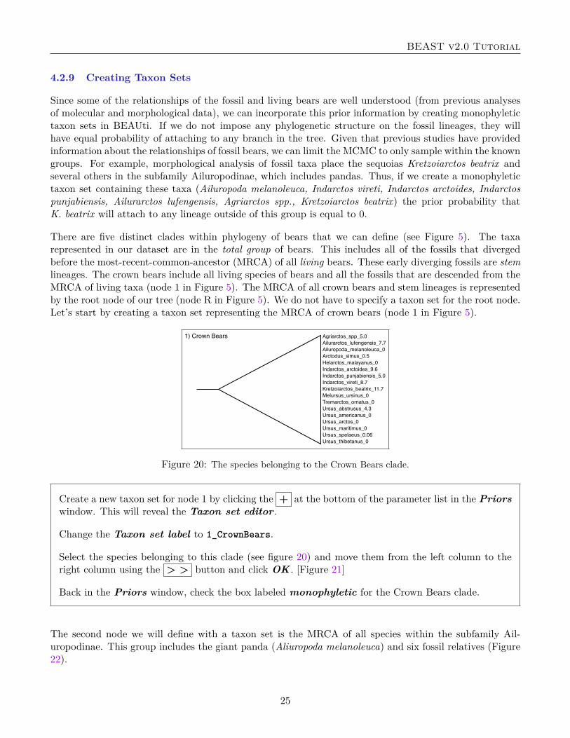
There are five distinct clades within phylogeny of bears that we can define (see Figure 5). The taxarepresented in our dataset are in the total group of bears. This includes all of the fossils that divergedbefore the most-recent-common-ancestor (MRCA) of all living bears. These early diverging fossils are stemlineages. The crown bears include all living species of bears and all the fossils that are descended from theMRCA of living taxa (node 1 in Figure 5). The MRCA of all crown bears and stem lineages is representedby the root node of our tree (node R in Figure 5). We do not have to specify a taxon set for the root node.Let’s start by creating a taxon set representing the MRCA of crown bears (node 1 in Figure 5).
Agriarctos_spp_5.0
Ailurarctos_lufengensis_7.7
Ailuropoda_melanoleuca_0
Arctodus_simus_0.5
Helarctos_malayanus_0
Indarctos_arctoides_9.6
Indarctos_punjabiensis_5.0
Indarctos_vireti_8.7
Kretzoiarctos_beatrix_11.7
Melursus_ursinus_0
Tremarctos_ornatus_0
Ursus_abstrusus_4.3
Ursus_americanus_0
1) Crown Bears
Ursus_arctos_0
Ursus_maritimus_0
Ursus_spelaeus_0.06
Ursus_thibetanus_0
Figure 20: The species belonging to the Crown Bears clade.
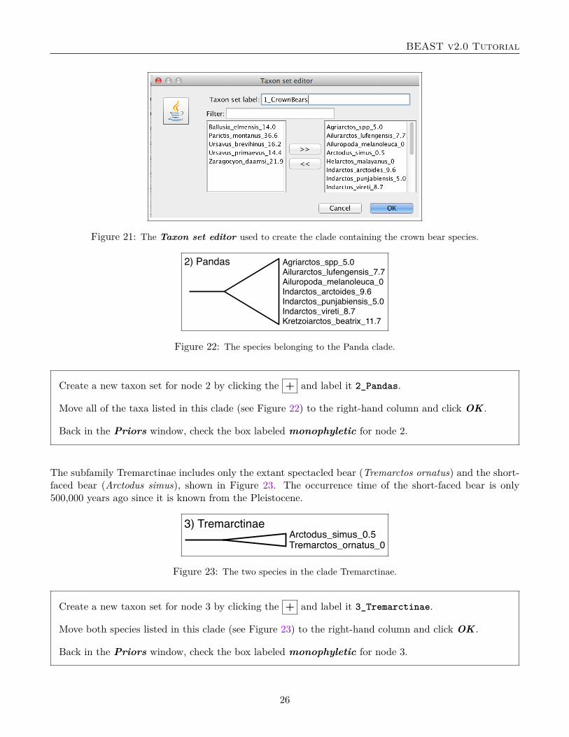
Create a new taxon set for node 1 by clicking the + at the bottom of the parameter list in the Priorswindow. This will reveal the Taxon set editor .
Change the Taxon set label to 1_CrownBears.
Select the species belonging to this clade (see figure 20) and move them from the left column to theright column using the > > button and click OK . [Figure 21]
Back in the Priors window, check the box labeled monophyletic for the Crown Bears clade.
The second node we will define with a taxon set is the MRCA of all species within the subfamily Ail-uropodinae. This group includes the giant panda (Aliuropoda melanoleuca) and six fossil relatives (Figure22).
25
BEAST v2.0 Tutorial
Figure 21: The Taxon set editor used to create the clade containing the crown bear species.
Figure 22: The species belonging to the Panda clade.
Create a new taxon set for node 2 by clicking the + and label it 2_Pandas.
Move all of the taxa listed in this clade (see Figure 22) to the right-hand column and click OK .
Back in the Priors window, check the box labeled monophyletic for node 2.
The subfamily Tremarctinae includes only the extant spectacled bear (Tremarctos ornatus) and the short-faced bear (Arctodus simus), shown in Figure 23. The occurrence time of the short-faced bear is only500,000 years ago since it is known from the Pleistocene.
Arctodus_simus_0.5Tremarctos_ornatus_0
3) Tremarctinae
Figure 23: The two species in the clade Tremarctinae.
Create a new taxon set for node 3 by clicking the + and label it 3_Tremarctinae.
Move both species listed in this clade (see Figure 23) to the right-hand column and click OK .
Back in the Priors window, check the box labeled monophyletic for node 3.
26
BEAST v2.0 Tutorial
The subfamily Ursinae comprises all of the species in the genus Ursus (including two fossil species) as wellas the sun bear (Helarctos malayanus) and the sloth bear (Melursus ursinus). These species are listed inFigure 24.
4) Ursinae Helarctos_malayanus_0
Melursus_ursinus_0
Ursus_abstrusus_4.3
Ursus_americanus_0
Ursus_arctos_0
Ursus_maritimus_0
Ursus_spelaeus_0.06
Ursus_thibetanus_0
Figure 24: The species belonging to the subfamily Ursinae.
Create a new taxon set for node 4 by clicking the + and label it 4_Ursinae.
Move all of the taxa listed in this clade (see Figure 24) to the right-hand column and click OK .
Back in the Priors window, check the box labeled monophyletic for node 4.
Finally, multiple studies using molecular data have shown that the polar bear (Ursus maritimus) and thebrown bear (Ursus arctos) are closely related. Furthermore, phylogenetic analyses of ancient DNA fromPleistocene sub-fossils concluded that the cave bear (Ursus spelaeus) is closely related to the polar bearand the brown bear (Figure 25).
Ursus_arctos_0
Ursus_maritimus_0
Ursus_spelaeus_0.06
5) Brown Bears
Figure 25: Three closely related Ursus species in the “Brown Bears” clade.
Create a new taxon set for node 5 by clicking the + and label it 5_BrownBears.
Move all of the taxa listed in this clade (see Figure 25) to the right-hand column and click OK .
Back in the Priors window, check the box labeled monophyletic for node 5.
At this point, there should be five, monophyletic taxon sets listed in the Priors window.
4.2.10 Other BEAUti Options
There are two additional windows that are hidden in BEAUti by default. You can reveal them by selectingView ⇒View All from the pull-down menu above. This will reveal the Initialization and Operatorspanels. The Initialization options allow you to change the starting values for the various parameters andspecify if you want them estimated or fixed. The Operators menu contains a list of the parameters and
27
BEAST v2.0 Tutorial
hyperparameters that will be sampled over the course of the MCMC run. In this window, it is possible toturn off any of the elements listed to fix a given parameter to its starting value. For example, if you wouldlike to estimate divergence times on a fixed tree topology (using a starting tree that you provided), thendisable proposals operating on the Tree. For this exercise, leave both windows unmodified.
4.2.11 Set MCMC Options and Save the XML File
Navigate to the MCMC window.
Now that you have specified all of your data elements, models, priors, and operators, go to the MCMCtab to set the length of the Markov chain, sample frequency, and file names. By default, BEAST sets thenumber of generations to 10,000,000.
Since we have a limited amount of time for this exercise, change the Chain Length to 2,000,000.(Runtimes may vary depending on your computer, if you have reason to believe that this may take avery long time, then change the run length to something smaller.)
Next we can set the filenames and output frequency.
Reveal the options for the tracelog using the ▶ to the left.
The frequency parameters are sampled and logged to file can be altered in the box labeled Log Every.In general, this value should be set relative to the length of the chain to avoid generating excessively largeoutput files. If a low value is specified, the output files containing the parameter values and trees will bevery large, possibly without gaining much additional information. Conversely, if you specify an exceedinglylarge sample interval, then you will not get enough information about the posterior distributions of yourparameters.
Change Log Every to 100. Also specify a name for the log file by changing File Name tobearsDivtime_FBD.log.
Next, we will specify how the trees are written to file. Analyses in BEAST often estimate parameters thatare associated with each branch in the tree (i.e, substitution rate). Additionally, the tree topology andbranching times for each MCMC iteration can be written to file. These parameters are stored in a differentfile with the trees written in extended Newick format. The default name for this file is $(tree).trees.The string “$(tree)” indicates the name of the tree we defined in the Partitions panel. For this analysiswe relabeled this variable: bearsTree and our file name will begin with bearsTree even if we do not alterthe name of this file.
28
BEAST v2.0 Tutorial
Reveal the options for the treelog.t:bearsTree file. Keep the File Name $(tree).1.trees and LogEvery to 100.
Note that both files have the digit 1 in the file name. That is because we intend to run this analysismultiple times. An important part of any MCMC analysis is that multiple, independent runs are executedstarting from different initial states for the various parameters. To do this, one can create multiple files inBEAUti, ensuring that the log and trees files have different names; or you can simply copy the XML fileand alter the file names and starting states in a text editor. Given the time available for this practical, itisn’t feasible to run multiple chains, but the output will be provided for you to evaluate this.
Now we are ready to save the XML file!
In the pull-down menu save the file by going to File ⇒Save As and save the file:bearsDivtime_FBD.xml.
For the last step in BEAUti, create an XML file that will run the analysis by sampling under the prior.This means that the MCMC will ignore the information coming from the sequence data and only sampleparameters in proportion to their prior probability. The output files produced from this run will providea way to visualize the marginal prior distributions on each parameter.
Check the box labeled Sample From Prior at the bottom of the MCMC panel. Wewill want to change the names of the output files as well, so change the tracelog –File Name to bearsDivtime_FBD.prior.log and the treelog.t:bearsTree – File Name tobearsDivtime_FBD.prior.trees.
Save these changes by going to File ⇒Save As and name the file bearsDivtime_FBD.prior.xml.
4.3 Making changes in the XML file
BEAUti is a great tool for generating a properly-formatted XML file for many types of BEAST analyses.However, you may encounter errors that require modifying elements in your input file and if you wish tomake small to moderate changes to your analysis, altering the input file is far less tedious than generatinga new one using BEAUti. Furthermore, BEAST is a rich program and all of the types of analyses, models,and parameters available in the core cannot be specified using BEAUti. Thus, some understanding of theBEAST XML format is essential.
Open the bearsDivtime_FBD.xml file generated by BEAUti in your text editor and glance over thecontents. BEAUti provides many comments describing each of the elements in the file.
As you look over the contents of this file, you will notice that the components are specified in an ordersimilar to the steps you took in BEAUti. The XML syntax is very verbose. This feature makes it fairly
29
BEAST v2.0 Tutorial
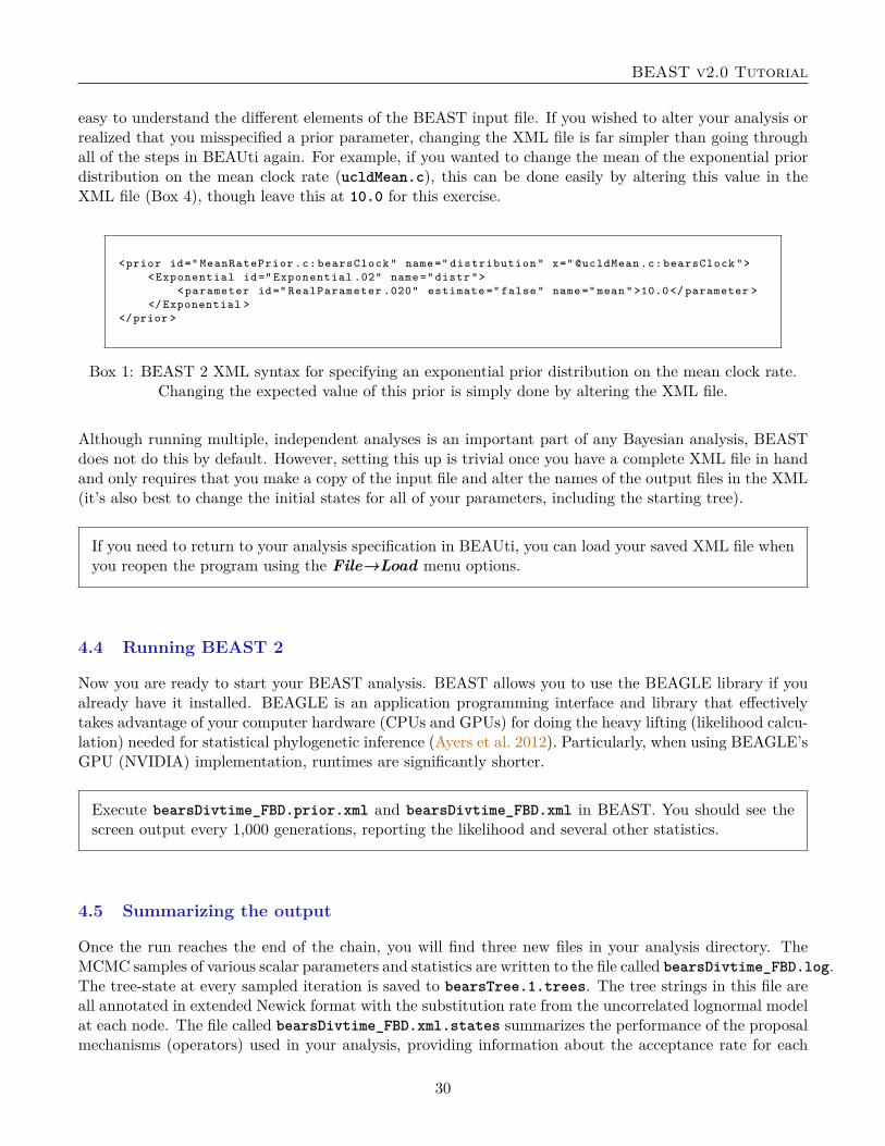
easy to understand the different elements of the BEAST input file. If you wished to alter your analysis orrealized that you misspecified a prior parameter, changing the XML file is far simpler than going throughall of the steps in BEAUti again. For example, if you wanted to change the mean of the exponential priordistribution on the mean clock rate (ucldMean.c), this can be done easily by altering this value in theXML file (Box 4), though leave this at 10.0 for this exercise.
<prior id =" MeanRatePrior .c: bearsClock " name =" distribution " x=" @ucldMean .c: bearsClock "><Exponential id =" Exponential .02" name =" distr ">
<parameter id =" RealParameter .020" estimate =" false " name =" mean " >10.0 </ parameter ></ Exponential >
</prior >
Box 1: BEAST 2 XML syntax for specifying an exponential prior distribution on the mean clock rate.Changing the expected value of this prior is simply done by altering the XML file.
Although running multiple, independent analyses is an important part of any Bayesian analysis, BEASTdoes not do this by default. However, setting this up is trivial once you have a complete XML file in handand only requires that you make a copy of the input file and alter the names of the output files in the XML(it’s also best to change the initial states for all of your parameters, including the starting tree).
If you need to return to your analysis specification in BEAUti, you can load your saved XML file whenyou reopen the program using the File→Load menu options.
4.4 Running BEAST 2
Now you are ready to start your BEAST analysis. BEAST allows you to use the BEAGLE library if youalready have it installed. BEAGLE is an application programming interface and library that effectivelytakes advantage of your computer hardware (CPUs and GPUs) for doing the heavy lifting (likelihood calcu-lation) needed for statistical phylogenetic inference (Ayers et al. 2012). Particularly, when using BEAGLE’sGPU (NVIDIA) implementation, runtimes are significantly shorter.
Execute bearsDivtime_FBD.prior.xml and bearsDivtime_FBD.xml in BEAST. You should see thescreen output every 1,000 generations, reporting the likelihood and several other statistics.
4.5 Summarizing the output
Once the run reaches the end of the chain, you will find three new files in your analysis directory. TheMCMC samples of various scalar parameters and statistics are written to the file called bearsDivtime_FBD.log.The tree-state at every sampled iteration is saved to bearsTree.1.trees. The tree strings in this file areall annotated in extended Newick format with the substitution rate from the uncorrelated lognormal modelat each node. The file called bearsDivtime_FBD.xml.states summarizes the performance of the proposalmechanisms (operators) used in your analysis, providing information about the acceptance rate for each
30
BEAST v2.0 Tutorial
move. Reviewing this file can help identify operators that might need adjustment if their acceptanceprobabilities are too high.
The main output files are the .log file and .trees file. It is not feasible to review the data contained inthese files by simply opening them in a spreadsheet program or a tree viewing program. Fortunately, thedevelopers of BEAST have also written general utility programs for summarizing and visualizing posteriorsamples from Bayesian inference using MCMC. Tracer is a cross-platform, java program for summarizingposterior samples of scaler parameters. This program is necessary for assessing convergence, mixing, anddetermining an adequate burn-in. Tree topologies, branch rates, and node heights are summarized usingthe program TreeAnnotator and visualized in FigTree.
4.5.1 Tracer
This section will briefly cover using Tracer and visual inspection of the analysis output for MCMC conver-gence diagnostics.
Open Tracer and import the bearsDivtime_FBD.log file in the File→Import New Trace File.
The fist statistic loaded will be the posterior , in the Estimates tab, and you can see the list of statisticsand variables that you can navigate through and visualize the summaries. You may notice that items inthe ESS column are colored red or gold. The MCMC runs you have performed today are far too shortto produce adequate posterior estimates of divergence times and substitution model parameters and thisis reflected in the ESS values. The ESS is the effective sample size of a parameter. The value indicatesthe number of effectively independent draws from the posterior in the sample. This statistic can help toidentify autocorrelation in your samples that might result from poor mixing. It is important that you runyour chains long enough and sufficiently sample the stationary distribution so that the ESS values of yourparameters are all high (over 200 or so).
Click on a parameter with a low ESS and explore the various windows in Tracer. It is clear that wemust run the MCMC chain longer to get good estimates.
Provided with the files for this exercise are the output files from analyses run for 50,000,000 iterations.The files can be found in the output directory and are all labeled with the file stem: bearsDivtime* andbearsTree*.
Close bearsDivtime_FBD.log in Tracer using the - button and open bearsDivtime.1.log,bearsDivtime.2.log and bearsDivtime.prior.log.
These log files are from much longer runs and since we ran two independent, identical analyses, we cancompare the log files in Tracer and determine if they have converged on the same stationary distribution.Additionally, analyzing samples from the prior allows you to compare your posterior estimates to the priordistributions used for each parameter.
31
BEAST v2.0 Tutorial
Select and highlight all three files (bearsDivtime.1.log, bearsDivtime.2.log andbearsDivtime.prior.log) in the Trace Files pane (do not include Combined). This allows you tocompare all three runs simultaneously. Click on the various parameters and view how they differ intheir estimates and 95% credible intervals for those parameters
The 95% credible interval is a Bayesian measure of uncertainty that accounts for the data. If we use the95% credible interval, this means that the probability the true value of a parameter lies within this intervalis 0.95, given our model and data. This measure is often used to approximate the 95% highest posteriordensity region (HPD).
Find the parameter ucldStdev and compare the estimates of the standard deviation of the uncorrelatedlog-normal distribution.
The ucldStdev indicates the amount of variation in the substitution rates across branches. Our prior onthis parameter is an exponential distribution with ν = 2.997 (mean = 0.3337). Thus, there is a considerableamount of prior weight on ucldStdev = 0. A standard deviation of 0 indicates support for no variation insubstitution rates and the presence of a molecular clock.
With ucldStdev highlighted for all three runs, go to the Marginal Prob Distribution window,which allows you to compare the marginal posterior densities for each parameter. (By default Tracergives the kernel density estimate (KDE) of the marginal density. You can change this to a Histogramusing the options at the bottom of the window.)
Color (or “colour”) the densities by Trace File next to Colour by at the bottom of the window (ifyou do not see this option, increase the size of your Tracer window). You can also add a Legend toreveal which density belongs to which run file. [Figure 26]
The first thing you will notice from this plot is that the marginal densities from each of our analysisruns (bearsDivtime.1.log and bearsDivtime.2.log) are nearly identical. If you click through the othersampled parameters, these densities are the same for each one. This indicates that both of our runs haveconverged on the same stationary distribution. If some of the other parameters might not have mixed well,we may want to run them longer, but we can have good confidence that our runs have sampled the samedistribution.
Second, it is likely for the UCLD rates that the parameters of this model appear to be somewhat sensitiveto the priors. That is because we have several lineages in our tree without any data since we are usingfossils to calibrate under the FBD model. For these branches, the clock rate assigned to them is sampledfrom the prior. The branches with extant descendants, however have rates that are informed by DNAsequence data. Because of this implementation, it is difficult to visualize the branch rates and associatedparameters from the log files. If these parameters are of interest, then it may be necessary to extract therates associated with the extant branches from the MCMC samples of trees. When fossils are used withoutcharacter data, alternative implementations of the FBD model consider the fossils separately and thus, thebranch rates can be summarized for only the extant lineages (Heath et al. 2014).
32
BEAST v2.0 Tutorial
Figure 26: Comparing the marginal densities (using the kernel density estimate) of the ucldStdev parameter from2 independent runs (red and blue) and the prior (gray) in Tracer.
Next, we will look at the Marginal Prob Distribution for the turnover parameter (turnoverFBD).
Select all trace files for the turnoverFBD parameter and go to the Marginal Prob Distributionwindow.
Color the densities by TraceFile and add a legend. [Figure 27]
Figure 27: Comparing the marginal densities (using the histogram) of the turnoverFBD parameter from 2 inde-pendent runs (red and blue) and the prior (gray) in Tracer.
When comparing the MCMC with data to those sampled just under the prior, we can see that this priorand posterior densities are nearly identical. Additionally, you may be alarmed that the prior density looks
33
BEAST v2.0 Tutorial
nothing like the Uniform(0,1) prior we applied in BEAUti. However, it’s important to understand thatwhen specifying Sample From Prior in BEAUti we are telling BEAST to ignore the likelihood comingfrom the sequence data, but the MCMC continues to account for the other data—fossil occurence times—that we have input. Thus, since we have a good number of fossils, the estimates of turnover, diversification,and the sampling proportion are highly informed by these data. If we used fewer fossils, the posterior andprior densities would be much less congruent.
Continue examining the options in Tracer. This program is very, very useful for exploring many aspectsof your analysis.
4.5.2 Summarizing the Trees in Treeannotator
After reviewing the trace files from the two independent runs in Tracer and verifying that both runsconverged on the posterior distributions and reached stationarity, we can combine the sampled trees intoa single tree file and summarize the results.
Open the program LogCombiner and set the File type to Tree Files. Next, import the two tree filesin the output directory (bearsTree.1.trees and bearsTree.2.trees) using the + button.
Set a burn-in percentage of 20 for each file, thus discarding the first 20% of the samples in each treefile.
Click on the Choose file ... button to create an output file and run the program. Name the file:bearsDivtime.combined.trees.
Once LogCombiner has terminated, you will have a file containing 40,000 trees which can be summarizedusing TreeAnnotator. TreeAnnotator takes a collection of trees and summarizes them by identifying thetopology with the best support, calculating clade posterior probabilities, and calculating 95% credibleintervals for node-specific parameters. All of the node statistics are annotated on the tree topology foreach node in the Newick string.
Open the program TreeAnnotator. Since we already discarded a set of burn-in trees when combiningthe tree files, we can leave Burnin set to 0 (though, if TreeAnnotator is taking a long time to loadthe trees, set the burnin to 10–60% to reduce the number of trees).
For the Target tree type, choose Maximum clade credibility tree.
The Maximum clade credibility tree is the topology with the highest product of clade posterior prob-abilities across all nodes. Alternatively, you can select the Maximum sum of clade credibilities whichsums all of the clade posteriors. Or you can provide a target tree from file. The Posterior probabilitylimit option applies to summaries on a target tree topology and only calculates posteriors for nodes thatare above the specified limit.
34
BEAST v2.0 Tutorial
Choose Median heights or Mean heights for Node heights which will set the node heights of theoutput tree to equal the median or mean height for each node in the sample of trees.
Choose bearsDivtime.combined.trees as your Input Tree File. Then name the Output File:bearsDivtime.summary.tre and click Run.
4.5.3 Visualizing the Dated Tree
The tree file produced by TreeAnnotator contains the maximum clade credibility tree and is annotatedwith summaries of the various parameters.
Open bearsDivtime.summary.tre in your text editor. The tree is written in NEXUS format. Lookat the tree string and notice the annotation. Each node in the tree is labeled with comments using the[¶meter_name=<value>] format.
The summary tree and it’s annotations can be visualized in the program FigTree.
Execute FigTree and open the file bearsDivtime.summary.tre.
Explore the options for viewing different summary statistics on the tree.
FigTree is a great tree-viewing program and it also allows you to produce publication-quality tree figures.However, viewing a dated phylogenetic tree with a unit-less timescale is not as meaningful as plotting thetree with a geological (stratigraphic) time scale. The R package strap (Bell and Lloyd 2014) offers severalnice functions for visualizing time-calibrated phylogenies in the context of the rock record.
Begin by opening R and load the strap package.
> library (" strap ")
Now we can read in the tree using the ape function read.nexus() (note that you might have to typein the whole file path to your tree).
> tree <- read.nexus (" bearsTree . summary .tre ")
In order to use the geoscalePhylo() function of strap, we have to set a value for the variabletree$root.time, which is the age of the root. We can compute this from the tree using thedist.nodes() function from ape:
You will notice that the plotted figure might need some work to make it easier to read taxon labels, etc.Additionally, we don’t get the node bars or other summary statistics for our tree. If we wish to plot thesevalues, then we need to do a bit more in R. With additional packages and functions, we can produce asummary tree that includes the credible intervals on the node ages (only for nodes in the extant tree,the origin time, and symbols representing the posterior probabilities of the tree bipartitions). This tree isshown in Figure 28 and the R syntax for producing this figure is provided in the output directory in thedownload files (plot_geoscaled_tree.R).
Figure 28: The maximum clade credibility tree summarized by TreeAnnotator and plotted with a geological timescale using the strap package in R. The fossil taxa are all indicated with an X in the taxon names. The ■ representsthe mean origin time. The remaining internal nodes of the tree are indicated with circles, where circles mark nodeswith posterior probability: ≥ 0.95, 0.95 > #≥ 0.75, 0.75 > #. The 95% credible intervals for node ages are shownwith transparent bars, for only nodes that are represented in the extant tree.
The tree shown in Figure 28 has several fossil taxa with zero-length branches, e.g., Parictis montanus and
36
BEAST v2.0 Tutorial
Ursus abstrusus. These branches actually indicate fossil taxa with a significant probability of representinga sampled ancestor. However, it is difficult to represent this in typical tree-viewing programs. A tree withsampled ancestors properly represented will have two-degree nodes — i.e., a node with only one descendant.The web-based tree viewer IcyTree (by Tim Vaughan) is capable of plotting such trees, although tools foreasily converting fully bifurcating trees to one with sampled ancestors are currently unavailable.
Although the tree in Figure 28 looks awesome, it can be misleading for this particular analysis. Sincewe did not provide character data for our 14 fossil taxa, the tree topology summarized in Figure 28does not adequately illustrate the degree of uncertainty in the phylogenetic relationships of the fossillineages. Without data, the fossil lineages can attach to any lineage on the tree that is consistent withthe monophyletic clades we specified and the fossil occurrence times with equal probability. Thus, therelationships shown here are not reliable as phylogenetic inferences. However, if we provided morphologicalcharacter data for these fossils, then this tree would be an adequate way to summarize our MCMC sampleof trees.
Since the fossil taxa were used in this analysis to only inform the fossilized birth-death model, we canprune off all of the fossil lineages and plot the tree with the geological time scale. An accessory pro-gram written by Alexandra Gavryushkina called Full2ExtantConvertor.jar is included in the downloadfiles. This program can be used to prune the fossil lineages off of the MCMC sample of trees (in filebearsDivtime.combined.trees), then use TreeAnnotator to summarize these trees. When executing theFull2ExtantConvertor.jar program, use a threshold value of 1e-5. This accounts for the rounding errorin branch lengths so that the program knows which taxa are considered extant. When the fossil lineages areremoved, much of the information about the history of this group is lost (Figure 29). However, alternativeapproaches for summarizing fossilized birth-death trees are currently under development.
01020304050Y
pres
ian
Lute
tian
Bar
toni
an
Pria
boni
an
Rup
elia
n
Cha
ttian
Aqu
itani
an
Bur
diga
lian
Lang
hian
Ser
rava
llian
Tort
onia
n
Mes
sini
an
Zan
clea
nP
iace
nzia
nG
elas
ian
Cal
abria
nM
iddl
eU
pper
Eoc
ene
Olig
ocen
e
Mio
cene
Plio
cene
Ple
isto
cene
Hol
ocen
e
Paleogene Neogene Quat.
Ailuropoda melanoleuca
Tremarctos ornatus
Melursus ursinus
Ursus arctos
Ursus maritimus
Helarctos malayanus
Ursus americanus
Ursus thibetanus
●
●
●
●
●
●
●
Figure 29: The maximum clade credibility tree of extant bears summarized by TreeAnnotator and plotted againststratigraphy using the strap package in R. The internal nodes of the tree are indicated with circles, where circlesmark nodes with posterior probability: ≥ 0.95, 0.95 > #≥ 0.75, 0.75 > #. The 95% credible intervals for nodeages are shown with transparent blue bars.
• Bayesian Evolutionary Analysis with BEAST 2 (Drummond and Bouckaert 2014)• BEAST 2 website and documentation: http://www.beast2.org/• BEAST 1 website and documentation: http://beast.bio.ed.ac.uk• Join the BEAST user discussion: http://groups.google.com/group/beast-users• RevBayes: https://github.com/revbayes/code• DPPDiv: https://github.com/trayc7/FDPPDIV• PhyloBayes: www.phylobayes.org/• multidivtime: http://statgen.ncsu.edu/thorne/multidivtime.html• MCMCtree (PAML): http://abacus.gene.ucl.ac.uk/software/paml.html• BEAGLE: http://code.google.com/p/beagle-lib/• A list of programs: http://evolution.genetics.washington.edu/phylip/software.html• The Paleobiology Database: http://www.paleodb.org• The Fossil Calibration Database: http://fossilcalibrations.org
This tutorial was written by Tracy Heath (with helpful contributions from Alexandra Gavryushk-ina and Rachel Warnock) for workshops on applied phylogenetics and molecular evolution and is licensedunder a Creative Commons Attribution 4.0 International License. Some content is based on the DivergenceDating Tutorial with BEAST 2.0 by Drummond, Rambaut, and Bouckaert.
Abella, J, P Montoya, and J Morales. 2011. Una nueva especie de Agriarctos (Ailuropodinae, Ursidae,Carnivora) en la localidad de Nombrevilla 2 (Zaragoza, España). Estudios Geológicos 67: 187–191.
Abella, J, DM Alba, JM Robles, A Valenciano, C Rotgers, R Carmona, P Montoya, and J Morales. 2012.Kretzoiarctos gen. nov., the oldest member of the giant panda clade. PLoS One 17: e48985.
Aldous, D. 2001. Stochastic models and descriptive statistics for phylogenetic trees, from Yule to today.Statistical Science 16: 23–34.
Aldous, D and L Popovic. 2005. A critical branching process model for biodiversity. Advances in AppliedProbability 37: 1094–1115.
Andrews, P and H Tobien. 1977. New Miocene locality in turkey with evidence on the origin of Ramap-ithecus and Sivapithecus. Nature 268: 699.
Aris-Brosou, S and Z Yang. 2003. Bayesian models of episodic evolution support a late precambrian explo-sive diversification of the Metazoa. Molecular Biology and Evolution 20: 1947–54.
— 2002. Effects of models of rate evolution on estimation of divergence dates with special reference to theMetazoan 18S ribosomal RNA phylogeny. Systematic Biology 51: 703–714.
Ayers, DL et al. 2012. BEAGLE: an application programming interface and high-performance computinglibrary for statistical phylogenetics. Systematic Biology 61: 170–173.
Baele, G, WLS Li, AJ Drummond, MA Suchard, and P Lemey. 2013. Accurate model selection of relaxedmolecular clocks in Bayesian phylogenetics. Molecular Biology and Evolution 30: 239–243.
Baele, G, P Lemey, T Bedford, A Rambaut, MA Suchard, and AV Alekseyenko. 2012. Improving theaccuracy of demographic and molecular clock model comparison while accommodating phylogeneticuncertainty. Molecular Biology and Evolution 30: 2157–2167.
Baryshnikov, GF. 2002. Late Miocene Indarctos punjabiensis atticus (Carnivora, Ursidae) in Ukraine withsurvey of Indarctos records from the former USSR. Russian J. Theriol 1: 83–89.
Bell, MA and GT Lloyd. 2014. Strap: an R package for plotting phylogenies against stratigraphy andassessing their stratigraphic congruence. Palaeontology
Benton, MJ and FJ Ayala. 2003. Dating the tree of life. Science 300: 1698–1700.Benton, MJ, MA Wills, and R Hitchin. 2000. Quality of the fossil record through time. Nature 403: 534–
537.Bjork, PR. 1970. The Carnivora of the Hagerman local fauna (late Pliocene) of Southwestern idaho.
Transactions of the American Philosophical Society 60: 3–54.Bouckaert, R, J Heled, D Kühnert, T Vaughan, CH Wu, D Xie, MA Suchard, A Rambaut, and AJ
Drummond. 2014. Beast 2: a software platform for Bayesian evolutionary analysis. PLoS computationalbiology 10: e1003537.
Brown, R and Z Yang. 2011. Rate variation and estimation of divergence times using strict and relaxedclocks. BMC Evolutionary Biology 11: 271.
Churcher, C, A Morgan, and L Carter. 1993. Arctodus simus from the Alaskan Arctic slope. CanadianJournal of Earth Sciences 30: 1007–1013.
Clark, J and TE Guensburg. 1972. Arctoid Genetic Characters as Related to the Genus Parictis. Vol. 1150.Field Museum of Natural History, Chicago, Ill.
Cutler, DJ. 2000. Estimating divergence times in the presence of an overdispersed molecular clock. Molec-ular Biology and Evolution 17: 1647–1660.
— 2000. Understanding the overdispersed molecular clock. Genetics 154: 1403–1417.Darriba, D, AJ Aberer, T Flouri, TA Heath, F Izquierdo-Carrasco, and A Stamatakis. 2013. Boosting
the performance of Bayesian divergence time estimation with the phylogenetic likelihood library. IEEE27th International Symposium on Parallel & Distributed Processing doi:10.1109/IPDPSW.2013.267.
39
BEAST v2.0 Tutorial
dos Reis, M and Z Yang. 2012. The unbearable uncertainty of Bayesian divergence time estimation. Journalof Systematics and Evolution 51: 30–43.
dos Reis, M, J Inoue, M Hasegawa, R Asher, P Donoghue, and Z Yang. 2012. Phylogenomic datasets provideboth precision and accuracy in estimating the timescale of placental mammal phylogeny. Proceedingsof the Royal Society B: Biological Sciences 279: 3491–3500.
dos Reis, M and Z Yang. 2011. Approximate likelihood calculation on a phylogeny for Bayesian estimationof divergence times. Molecular Biology and Evolution 28: 2161–2172.
Doyle, JA and MJ Donoghue. 1993. Phylogenies and angiosperm diversification. Paleobiology 19: 141–167.Drummond, AJ and A Rambaut. 2007. BEAST: Bayesian evolutionary analysis by sampling trees. BMC
Evolutionary Biology 7: 214.Drummond, AJ and MA Suchard. 2010. Bayesian random local clocks, or one rate to rule them all. BMC
Biology 8: 114.Drummond, AJ, SY Ho, MJ Phillips, and A Rambaut. 2006. Relaxed phylogenetics and dating with
confidence. PLoS Biology 4: e88.Drummond, AJ and RR Bouckaert. 2014. Bayesian evolutionary analysis with BEAST 2. Cambridge Uni-
versity Press,Drummond, AJ, OG Pybus, A Rambaut, R Forsberg, and AG Rodrigo. 2003. Measurably evolving popu-
lations. Trends in Ecology & Evolution 18: 481–488.Fan, Y, R Wu, MH Chen, L Kuo, and PO Lewis. 2011. Choosing among partition models in Bayesian
phylogenetics. Molecular Biology and Evolution 28: 523–532.Foote, M. 1996. On the probability of ancestors in the fossil record. Paleobiology 22: 141–151.Gandolfo, MA, KC Nixon, and WL Crepet. 2008. Selection of fossils for calibration of molecular dating
models. Annals of the Missouri Botanical Garden 95: 34–42.Gaut, BA and BS Weir. 1994. Detecting substitution-rate heterogeneity among regions of a nucleotide
sequence. Molecular Biology and Evolution 11: 620–629.Gavryushkina, A, D Welch, T Stadler, and AJ Drummond. 2014. Bayesian inference of sampled ancestor
trees for epidemiology and fossil calibration. PLoS Computational Biology 10: e1003919.Geraads, D, T Kaya, S Mayda, et al. 2005. Late miocene large mammals from Yulafli, Thrace region,
Turkey, and their biogeographic implications. Acta Palaeontologica Polonica 50: 523–544.Gernhard, T. 2008. The conditioned reconstructed process. Journal of Theoretical Biology 253: 769–778.Ginsburg, L and J Morales. 1995. Zaragocyon daamsi n. gen. sp. nov., ursidae primitif du Miocène inférieur
d’Espagne. Comptes Rendus de l’Académie des Sciences. Série 2. Sciences de la Terre et des Planètes321: 811–815.
Ginsburg, L and J Morales. 1998. Les Hemicyoninae (Ursidae, Carnivora, Mammalia) et les formes ap-parentées du Miocène inférieur et moyen d’Europe occidentale. Annales de Paléontologie. 84: pp. 71–123.
Graur, D and W Martin. 2004. Reading the entrails of chickens: Molecular timescales of evolution and theillusion of precision. Trends in Genetics 20: 80–86.
Griffiths, R and S Tavare. 1994. Simulating probability distributions in the coalescent. Theoretical Popu-lation Biology 46: 131–159.
Guindon, S. 2010. Bayesian estimation of divergence times from large sequence alignments. MolecularBiology and Evolution 27: 1768–1781.
Hasegawa, M, H Kishino, and T Yano. 1985. Dating the human-ape splitting by a molecular clock ofmitochondrial DNA. Journal of Molecular Evolution 22: 160–174.
— 1989. Estimation of branching dates among primates by molecular clocks of nuclear DNA which sloweddown in Hominoidea. Journal of Human Evolution 18: 461–476.
Hastings, WK. 1970. Monte Carlo sampling methods using Markov chains and their applications. Biometrika57: 97–109.
40
BEAST v2.0 Tutorial
Heath, TA. 2012. A hierarchical Bayesian model for calibrating estimates of species divergence times.Systematic Biology 61: 793–809.
Heath, TA and BR Moore. Bayesian inference of species divergence times. Bayesian Phylogenetics: Meth-ods, Algorithms, and Applications. (Ed.) Chen, MH, Kuo, L, and Lewis, PO. Chapman & Hall/CRCMathematical and Computational Biology. Chapman & Hall/CRC, Boca Raton, FL, 277–318.
Heath, TA, MT Holder, and JP Huelsenbeck. 2012. A Dirichlet process prior for estimating lineage-specificsubstitution rates. Molecular Biology and Evolution 29: 939–255.
Heath, TA, DJ Zwickl, J Kim, and DM Hillis. 2008. Taxon sampling affects inferences of macroevolutionaryprocesses from phylogenetic trees. Systematic Biology 57: 160–166.
Heath, TA, SM Hedtke, and DM Hillis. 2008. Taxon sampling and the accuracy of phylogenetic analyses.Journal of Systematics and Evolution 46: 239–257.
Heath, TA, JP Huelsenbeck, and T Stadler. 2014. The fossilized birth-death process for coherent calibrationof divergence-time estimates. Proceedings of the National Academy of Sciences, USA 111: E2957–E2966.
Heibl, C. PHYLOCH: R language tree plotting tools and interfaces to diverse phylogenetic software pack-ages. http://www.christophheibl.de/Rpackages.html. 2008.
Heizmann, E, L Ginsburg, and C Bulot. 1980. Prosansanosmilus peregrinus, ein neuer machairodontiderFelidae aus dem Miozän Deutschlands und Frankreichs. Stuttgarter Beitr. Naturk. B 58: 1–27.
Heled, J and AJ Drummond. 2010. Bayesian inference of species trees from multilocus data. MolecularBiology and Evolution 27: 570–580.
— 2012. Calibrated tree priors for relaxed phylogenetics and divergence time estimation. Systematic Bi-ology 61: 138–149.
Heled, J and AJ Drummond. 2013. Calibrated birth-death phylogenetic time-tree priors for Bayesianinference. arXiv preprint arXiv:1311.4921
Himmelmann, L and D Metzler. 2009. Treetime: an extensible c++ software package for Bayesian phylogenyreconstruction with time-calibration. Bioinformatics 25: 2440–2441.
Ho, SYW. 2007. Calibrating molecular estimates of substitution rates and divergence times in birds. Journalof Avian Biology 38: 409–414.
Ho, SYW and MJ Phillips. 2009. Accounting for calibration uncertainty in phylogenetic estimation ofevolutionary divergence times. Systematic Biology 58: 367–380.
Ho, SYW, R Lanfear, L Bromham, MJ Phillips, J Soubrier, AG Rodrigo, and A Cooper. 2011. Time-dependent rates of molecular evolution. Molecular Ecology 20: 3087–3101.
Höhna, S and AJ Drummond. 2012. Guided tree topology proposals for Bayesian phylogenetic inference.Systematic Biology 61: 1–11.
Höhna, S, T Stadler, F Ronquist, and T Britton. 2011. Inferring speciation and extinction rates underdifferent sampling schemes. Molecular Biology and Evolution 28: 2577–2589.
Huelsenbeck, JP, B Larget, and DL Swofford. 2000. A compound Poisson process for relaxing the molecularclock. Genetics 154: 1879–1892.
Hug, LA and AJ Roger. 2007. The impact of fossils and taxon sampling on ancient molecular datinganalyses. Molecular Biology and Evolution 24: 1889–1897.
Hugall, AF, R Foster, and MSY Lee. 2007. Calibration choice, rate smoothing, and the pattern of tetrapoddiversification according to the long nuclear gene RAG-1. Systematic Biology 56: 543–63.
Hull, DL. 1988. Science as a Process. An Evolutionary Account of the Social and Conceptual Developmentof Science. University of Chicago Press, Chicago.
Inoue, J, PC Donoghue, and Z Yang. 2010. The impact of the representation of fossil calibrations onBayesian estimation of species divergence times. Systematic Biology 59: 74–89.
Jin, C, RL Ciochon, W Dong, RM Hunt, J Liu, M Jaeger, and Q Zhu. 2007. The first skull of the earliestgiant panda. Proceedings of the National Academy of Sciences 104: 10932–10937.
41
BEAST v2.0 Tutorial
Kendall, DG. 1948. On the generalized “birth-and-death” process. Annals of Mathematical Statistics 19:1–15.
Kingman, JFC. 1982. Exchangeability and the evolution of large populations. Exchangeability in Probabilityand Statistics. (Ed.) Koch, G and Spizzichino, F. North-Holland, pp. 97–112.
— 1982. On the genealogy of large populations. Essays in Statistical Science: Papers in Honour of P. A.P. Moran, Journal of Applied Probability, Special Volume 19A. (Ed.) Gani, J and Hannan, EJ. AppliedProbability Trust, pp. 27–43.
— 1982. The coalescent. Stochastic Processes and their Applications 13: 235–248.Kishino, H and M Hasegawa. 1990. Converting distance to time: Application to human evolution. Methods
in Enzymology 183: 550–570.Kishino, H, T Miyata, and M Hasegawa. 1990. Maximum likelihood inference of protein phylogeny and the
origin of chloroplasts. Journal of Molecular Evolution 31: 151–160.Kishino, H, JL Thorne, and W Bruno. 2001. Performance of a divergence time estimation method under
a probabilistic model of rate evolution. Molecular Biology and Evolution 18: 352–361.Krause, J, T Unger, A Noçon, AS Malaspinas, SO Kolokotronis, M Stiller, L Soibelzon, H Spriggs, PH
Dear, AW Briggs, et al. 2008. Mitochondrial genomes reveal an explosive radiation of extinct and extantbears near the Miocene-Pliocene boundary. BMC Evolutionary Biology 8: 220.
Landis, MJ, NJ Matzke, BR Moore, and JP Huelsenbeck. 2013. Bayesian analysis of biogeography whenthe number of areas is large. Systematic biology 789–804.
Lartillot, N. 2013. Interaction between selection and biased gene conversion in mammalian protein-codingsequence evolution revealed by a phylogenetic covariance analysis. Molecular Biology and Evolution 30:356–368.
Lartillot, N and F Delsuc. 2012. Joint reconstruction of divergence times and life-history evolution inplacental mammals using a phylogenetic covariance model. Evolution 66: 1773–1787.
Lartillot, N and R Poujol. 2011. A phylogenetic model for investigating correlated evolution of substitutionrates and continuous phenotypic characters. Molecular Biology and Evolution 28: 729–744.
Lee, MSY, PM Oliver, and MN Hutchinson. 2009. Phylogenetic uncertainty and molecular clock calibra-tions: A case study of legless lizards (Pygopodidae, Gekkota). Molecular Phylogenetics and Evolution50: 661–666.
Lemey, P, A Rambaut, AJ Drummond, and MA Suchard. 2009. Bayesian phylogeography finds its roots.PLoS Computational Biology 5: e1000520.
Lepage, T, D Bryant, H Philippe, and N Lartillot. 2007. A general comparison of relaxed molecular clockmodels. Molecular Biology and Evolution 24: 2669–2680.
Lepage, T, S Lawi, P Tupper, and D Bryant. 2006. Continuous and tractable models for the variation ofevolutionary rates. Mathematical Biosciences 199: 216–233.
Li, WLS and AJ Drummond. 2012. Model averaging and Bayes factor calculation of relaxed molecularclocks in Bayesian phylogenetics. Molecular Biology and Evolution 29: 751–761.
Lloyd, GT, JR Young, and AB Smith. 2012. Taxonomic structure of the fossil record is shaped by samplingbias. Systematic Biology 61: 80–89.
Loreille, O, L Orlando, M Patou-Mathis, M Philippe, P Taberlet, and C Hänni. 2001. Ancient DNA analysisreveals divergence of the cave bear, Ursus spelaeus, and brown bear, Ursus arctos, lineages. CurrentBiology 11: 200–203.
Lukoschek, V, JS Keogh, and JC Avise. 2012. Evaluating fossil calibrations for dating phylogenies in lightof rates of molecular evolution: A comparison of three approaches. Systematic Biology 61: 22–43.
Magallón, S. 2009. Using fossils to break long branches in molecular dating: A comparison of relaxed clocksapplied to the origin of angiosperms. Systematic Biology 59: 384–399.
Marshall, CR. 2008. A simple method for bracketing absolute divergence times on molecular phylogeniesusing multiple fossil calibration points. The American Naturalist 171: 726–742.
42
BEAST v2.0 Tutorial
Marshall, CR. 1990. Confidence intervals on stratigraphic ranges. Paleobiology 16: 1–10.Montoya, P, L Alcalá, and J Morales. 2001. Indarctos (Ursidae, Mammalia) from the Spanish Turolian
(Upper Miocene). Scripta Geologica 122: 123–151.Morlon, H, T Parsons, and J Plotkin. 2011. Reconciling molecular phylogenies with the fossil record.
Proceedings of the National Academy of Sciences 108: 16327–16332.Muse, SV and BS Weir. 1992. Testing for equality of evolutionary rates. Genetics 132: 269–276.Nee, S, RM May, and PH Harvey. 1994. The reconstructed evolutionary process. Philosophical Transactions
of the Royal Society B 344: 305–311.Nylander, J, J Wilgenbusch, D Warren, and D Swofford. 2008. Awty (are we there yet?): a system for
graphical exploration of mcmc convergence in Bayesian phylogenetics. Bioinformatics 24: 581.Parham, JF et al. 2012. Best practices for justifying fossil calibrations. Systematic Biology 61: 346–359.Popovic, L. 2004. Asymptotic genealogy of a critical branching process. Annals of Applied Probability 14:
2120–2148.Pyron, RA. 2011. Divergence time estimation using fossils as terminal taxa and the origins of Lissamphibia.
Systematic Biology 60: 466–481.Rambaut, A and L Bromham. 1998. Estimating divergence dates from molecular sequences. Molecular
Biology and Evolution 15: 442–448.Rannala, B and Z Yang. 2007. Inferring speciation times under an episodic molecular clock. Systematic
Biology 56: 453–466.— 1996. Probability distribution of molecular evolutionary trees: A new method of phylogenetic inference.
Journal of Molecular Evolution 43: 304–311.Revell, LJ. 2012. phytools: an R package for phylogenetic comparative biology (and other things). Methods
in Ecology and Evolution 3: 217–223.Robinson, M, M Gouy, C Gautier, and D Mouchiroud. 1998. Sensitivity of the relative-rate test to taxo-
nomic sampling. Molecular Biology and Evolution 15: 1091–1098.Rodrigo, AG, M Goode, R Forsberg, HA Ross, and A Drummond. 2003. Inferring evolutionary rates using
serially sampled sequences from several populations. Molecular Biology and Evolution 20: 2010–2018.Ronquist, F, S Klopfstein, L Vilhelmsen, S Schulmeister, DL Murray, and AP Rasnitsyn. 2012. A total-
evidence approach to dating with fossils, applied to the early radiation of the Hymenoptera. SystematicBiology 61: 973–999.
Rutschmann, F, T Eriksson, KA Salim, and E Conti. 2007. Assessing calibration uncertainty in moleculardating: the assignment of fossils to alternative calibration points. Systematic Biology 56: 591–608.
Sanderson, MJ. 1997. A nonparametric approach to estimating divergence times in the absence of rateconstancy. Molecular Biology and Evolution 14: 1218–1231.
— 2002. Estimating absolute rates of molecular evolution and divergence times: a penalized likelihoodapproach. Molecular Biology and Evolution 19: 101–109.
Shapiro, B, SYW Ho, AJ Drummond, MA Suchard, OG Pybus, and A Rambaut. 2011. A Bayesian phy-logenetic method to estimate unknown sequence ages. Molecular Biology and Evolution 28: 879–887.
Stadler, T. 2009. On incomplete sampling under birth-death models and connections to the sampling-basedcoalescent. Journal of Theoretical Biology 261: 58–66.
— 2010. Sampling-through-time in birth-death trees. Journal of Theoretical Biology 267: 396–404.— 2011. Simulating trees on a fixed number of extant species. Systematic Biology 60: 668–675.Stadler, T. 2011. Mammalian phylogeny reveals recent diversification rate shifts. Proceedings of the National
Academy of Sciences, USA 108: 6187–6192.Stadler, T, D Kühnert, S Bonhoeffer, and AJ Drummond. 2013. Birth–death skyline plot reveals temporal
changes of epidemic spread in HIV and hepatitis C virus (HCV). Proceedings of the National Academyof Sciences 110: 228–233.
43
BEAST v2.0 Tutorial
Suchard, MA, RE Weiss, and JS Sinsheimer. 2003. Testing a molecular clock without an outgroup: deriva-tions of induced priors on branch-length restrictions in a Bayesian framework. Systematic Biology 52:48–54.
Sukumaran, J and MT Holder. 2010. DendroPy: A Python library for phylogenetic computing. Bioinfor-matics 26: 1569–1571.
Tajima, F. 1993. Simple methods for testing molecular clock hypothesis. Genetics 135: 599–607.Thompson, EA. 1975. Human Evolutionary Trees. Cambridge University Press, Cambridge, England.Thorne, J and H Kishino. 2002. Divergence time and evolutionary rate estimation with multilocus data.
Systematic Biology 51: 689–702.Thorne, J, H Kishino, and IS Painter. 1998. Estimating the rate of evolution of the rate of molecular
evolution. Molecular Biology and Evolution 15: 1647–1657.Thorne, JL and H Kishino. 2005. Estimation of divergence times from molecular sequence data. Statistical
Methods in Molecular Evolution. (Ed.) Nielsen, R. Springer, New York, pp. 235–256.Thorpe, JP. 1982. The molecular clock hypothesis: biochemical evolution, genetic differentiation and sys-
tematics. Annual Review of Ecology and Systematics 13: 139–168.Warnock, RCM, Z Yang, and PCJ Donoghue. 2012. Exploring the uncertainty in the calibration of the
molecular clock. Biology Letters 8: 156–159.Warnock, RC, JF Parham, WG Joyce, TR Lyson, and PC Donoghue. 2015. Calibration uncertainty in
molecular dating analyses: there is no substitute for the prior evaluation of time priors. Proceedings ofthe Royal Society B: Biological Sciences 282: 20141013.
Weir, J and D Schluter. 2008. Calibrating the avian molecular clock. Molecular Ecology 17: 2321–2328.Welch, JJ, E Fontanillas, and L Bromham. 2005. Molecular dates for the “cambrian explosion”: the influence
of prior assumptions. Systematic Biology 54: 672–678.Wilkinson, RD, ME Steiper, C Soligo, RD Martin, Z Yang, and S Tavaré. 2011. Dating primate divergences
through an integrated analysis of palaeontological and molecular data. Systematic Biology 60: 16–31.Xie, W, PO Lewis, Y Fan, L Kuo, and MH Chen. 2011. Improving marginal likelihood estimation for
Bayesian phylogenetic model selection. Systematic Biology 60: 150–160.Yang, Z and B Rannala. 2006. Bayesian estimation of species divergence times under a molecular clock
using multiple fossil calibrations with soft bounds. Molecular Biology and Evolution 23: 212–226.— 1997. Bayesian phylogenetic inference using DNA sequences: A Markov chain Monte Carlo method.
Molecular Biology and Evolution 14: 717–724.Yang, Z and AD Yoder. 2003. Comparison of likelihood and Bayesian methods for estimating divergence
times using multiple gene loci and calibration points, with application to a radiation of cute-lookingmouse lemur species. Systematic Biology 52: 705–716.
Yoder, AD and Z Yang. 2000. Estimation of primate speciation dates using local molecular clocks. MolecularBiology and Evolution 17: 1081–1090.
Yule, GU. 1924. A mathematical theory of evolution, based on the conclusions of Dr. J. C. Wills, F. R. S.Philosophical Transactions of the Royal Society of London, Biology 213: 21–87.
Zuckerkandl, E and L Pauling. 1965. Evolutionary divergence and convergence in proteins. Evolving Genesand Proteins 97–166.
— 1962. Molecular disease, evolution, and genetic heterogeneity. Horizons in Biochemistry. (Ed.) Kasha,M and Pullman, B. Academic Press, New York, pp. 189–225.