Diversifying in the Integrated Markets of ASEAN+3 - A Quantitative Study of Stock Market Correlation Authors: Emelie Nordell Caroline Stark Supervisor: Anders Isaksson Student Umeå School of Business Spring semester 2010 Bachelor thesis, 15 hp
Transcript
Diversifying in the Integrated Markets of
ASEAN+3
- A Quantitative Study of Stock Market
Correlation
Authors: Emelie Nordell
Caroline Stark
Supervisor: Anders Isaksson Student Umeå School of Business Spring semester 2010
Bachelor thesis, 15 hp
I
Acknowledgement
Anders Isaksson, thank you for your support!
Linus Jansson, we dedicate our thesis to you.
II
Abstract There is evidence that globalization, economic assimilation and integration among
countries and their financial markets have increased correlation among stock markets
and the correlation may in turn impact investors’ allocation of their assets and economic
policies. We have conducted a quantitative study with daily stock index quotes for the
period January 2000 and December 2009 in order to measure the eventual correlation
between the markets of ASEAN+3. This economic integration consists of; Indonesia,
Malaysia, Philippines, Singapore, Thailand, China, Japan and South Korea. Our
problem formulation is:
Are the stock markets of ASEAN+3 correlated?
Does the eventual correlation change under turbulent market conditions?
In terms of the eventual correlation, discuss: is it possible to diversify an investment
portfolio within this area?
The purpose of the study is to conduct a research that will provide investors with
information about stock market correlation within the chosen market. We have
conducted the study with a positivistic view and a deductive approach with some
theories as our starting point. The main theories discussed are; market efficiency, risk
and return, Modern Portfolio Theory, correlation and international investments. By
using the financial datatbase, DataStream, we have been able to collect the necessary
data for our study. The data has been processed in the statistical program SPSS by using
Pearson correlation.
From the empirical findings and our analysis we were able to draw some main
conclusions about our study. We found that most of the ASEAN+3 countries were
strongly correlated with each other. Japan showed lower correlation with all of the other
countries. Based on this we concluded that economic integration seems to increase
correlation between stock markets. When looking at the economic downturn in 2007-
2009, we found that the correlation between ASEAN+3 became stronger and positive
for all of the countries. The results also showed that the correlation varies over time. We
concluded that it is, to a small extent, possible to diversify an investment portfolio
across these markets.
Keywords: integration, correlation, ASEAN+3, stock market index, Modern Portfolio
Theory, diversification
III
Table of Contents 1. Introduction .................................................................................................................. 1
1.1 Choice of Subject ................................................................................................... 2
1.2 Problem Background .............................................................................................. 2
1.3 Problem Formulation .............................................................................................. 5
The introductory chapter is focused on the problematic background of the thesis and the idea is to provide the reader with the basic tools concerning the thesis. Different stages of integration and basics about the ASEAN+3 will be presented in order to make the problem more comprehensive for the reader. The problem background is set to provide a suitable ground for the research question and the purpose of our study.
The purpose of the chapter is to give insight about the chosen subject and the problem concerned in our study.
"A whole has a beginning, a middle and an end"
- Aristoteles
2
1.1 Choice of Subject
In 1975, Balassa concluded that regional economic integration should be considered as
a policy tool for developing countries to increase economic development. He also wrote
that regional integration can benefit the member countries by allowing access to the
markets of their partners, reducing risk, making policy coordination easier and reducing
the cost of infant industry protection. (Balassa, 1975; 45) Ever since then, regional
economic integration seems to have expanded. NAFTA, EMU, MERCOSUR, AFTA,
CEPEA, TAFTA, GATT, APEC, the list with letter combinations over integrated
markets can go on forever. By reasoning we found that if a market is integrated a
possibility of correlation must exist.
We have decided to examine ASEAN+3, an economically integrated market in Asia
(clarification will be made in chapter 1.2). We found this market to be relevant for our
study, economic integration exists, something that we consider necessary in order to
carry out the intended research. Furthermore this is an emerging market in which we
believe investors are interested in and need more information about. The decision to
look at the Asian market was also based on an interest towards this emerging region of
the world. Considering the recent financial crisis we wanted to investigate a longer time
period in order to see if the correlation changes over time and under different market
conditions. The stock market development from January 2000 to December 2009 will
be used in the study.
1.2 Problem Background
During the last ten years international money and capital markets have become
increasingly integrated. The removal of restrictions on capital flow, floating exchange
rates, improved communications systems and new instruments are all factors that have
contributed to the process of integration. The deregulation has encouraged globalization
and integration which in turn creates a better access and a greater transparency of
information and pricing. (Palac-McMiken, 1997;299) As previously mentioned, there
are several markets in the world that have formed integration and before continuing we
want to clarify this concept by examining different stages of economic integration.
Preferential trade area (PTA)
This is the weakest form of economic integration. The member countries offer tariff
reductions to a limited set of partners in some product categories. The restrictions in
other product categories would remain. Usually the goal is to become a free trade area.
Free trade area (FTA)
When a group of countries agree to eliminate tariffs between themselves, but maintain
their own external tariffs on import from the rest of the world, they form a free trade
area. NAFTA, North American Free Trade Area is one example.
3
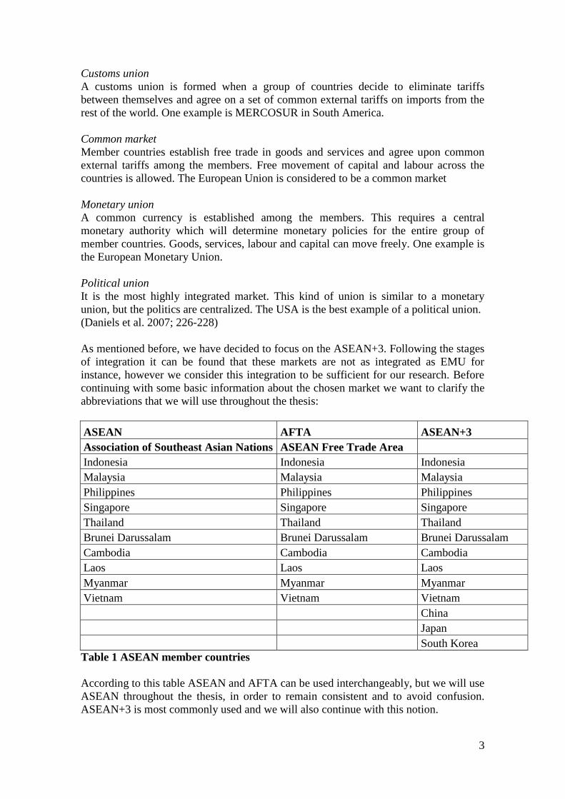
Customs union
A customs union is formed when a group of countries decide to eliminate tariffs
between themselves and agree on a set of common external tariffs on imports from the
rest of the world. One example is MERCOSUR in South America.
Common market
Member countries establish free trade in goods and services and agree upon common
external tariffs among the members. Free movement of capital and labour across the
countries is allowed. The European Union is considered to be a common market
Monetary union
A common currency is established among the members. This requires a central
monetary authority which will determine monetary policies for the entire group of
member countries. Goods, services, labour and capital can move freely. One example is
the European Monetary Union.
Political union
It is the most highly integrated market. This kind of union is similar to a monetary
union, but the politics are centralized. The USA is the best example of a political union.
(Daniels et al. 2007; 226-228)
As mentioned before, we have decided to focus on the ASEAN+3. Following the stages
of integration it can be found that these markets are not as integrated as EMU for
instance, however we consider this integration to be sufficient for our research. Before
continuing with some basic information about the chosen market we want to clarify the
abbreviations that we will use throughout the thesis:
ASEAN AFTA ASEAN+3
Association of Southeast Asian Nations ASEAN Free Trade Area
Does the eventual correlation change under turbulent market conditions?
In terms of the eventual correlation, discuss: is it possible to diversify an investment
portfolio within this area?
1.4 Purpose
The aim is to conduct a research that will provide investors with information about
stock market correlation within the chosen market. The main focus will be kept on the
possible correlation within the ASEAN+3 stock markets. By using a stock exchange
index of the member countries we aim to measure the degree of correlation. We also
intend to include an economic downturn to look at the possible effects it may have on
the correlation. From the results, investors interested in building a risk reduced portfolio
may be helped by our study of the ASEAN+3. Based on our findings we hope that they
will know more about how these markets move i.e. if they move together or not.
Hopefully, this information will help investors to draw conclusions about how to invest
their assets best.
1.5 Limitations
In order to keep the thesis comprehensive some limitations had to be made. First of all,
ASEAN consists of ten member countries, all of which is not equally developed. Due to
this problem we have limited the research in the number of countries. Since we are
using stock indexes as our tool to measure correlation a comprehensive index has to be
available. By browsing the internet we tried to find the stock markets for each country.
From this research we found that no functioning stock markets exist in Brunei
Darussalam, Cambodia, Laos and Myanmar. This made it impossible to include these
countries in our research. As previously discussed the most integrated markets within
the ASEAN are Indonesia, Malaysia, Philippines, Singapore and Thailand. All of these
five countries can thus be included, but what about Vietnam? On one hand a stock index
exists but on the other hand Vietnam’s integration with the other five countries is not
that strong. Based on this reasoning we have decided to exclude Vietnam. This
limitation may be criticised, however we have found some previous research that also
studied the five initial ASEAN member countries which we consider to strengthen our
argument.
In order to add scope in to our research we decided to include the +3 countries (China,
Japan and the South Korea). Furthermore we are investigating a long time period,
January 2000 to December 2009. Based on the chosen markets and the timeframe we
can see if correlation exists and whether it is stronger between the five ASEAN
countries compared to the +3 countries. We also include an economic downturn which
means that we can analyse the correlation under changing market conditions.
6
We have limited the data collection to one stock index per country and we will be using
daily stock index quotes (a database will be used to obtain the data). Eun and Shim
(1989) means that daily data series are appropriate for capturing potential interactions,
since a month or even a week may be long enough to obscure interactions that may last
only for a few days (Eun and Shim, 1989;242). Pearson correlation will be used in order
to analyse the relationship between the chosen variables and hence also detect the
degree of correlation (see chapter 5.1 through 5.3). We have chosen to only look at the
eventual correlation and the factors that may affect this have not been investigated
further, a limitation we had to make due to the time frame of the study.
7
2. Previous Research
The aim of this chapter is to provide the reader with a literature review in order to give an overview of what has been done within this field. The review was conducted with an intention to gain knowledge about what has been done, and hence also to detect a gap within the chosen research field. The purpose is to give the reader an insight of what has previously been done.
“The beginning of knowledge is the discovery of something we do not understand.”
- Frank Herbert
8
2.1 Literature Review
As previously mentioned, the countries explored in this thesis belong to an
economically integrated market and the underlying assumption is that this integration
would affect the correlation between these stock markets. When we reviewed previous
research within the same field we found that researchers have conducted various studies
concerning stock market correlation all over the world, on all kinds of markets,
integrated or not. To limit the review we have decided to focus on research mainly
conducted in the Asian market. The methods used in previous research have helped us
to develop our research in a beneficial way and also to avoid repeating history. Their
findings will also be discussed in comparison to our results. In a chronological order,
we will present some important researches in what we consider to be modern time.
Beginning in 1994, the relationship among the stock markets of four newly
industrialized economies (NIEs) in Asia, Japan and the USA was examined by
Chowdhury (1994). He used daily rates of return on the stock market indices from the
period January 1986 through December 1990 in a six-variable autoregressive (VAR)
model. The study revealed indications of significant linkages between the markets of
Hong Kong and Singapore and those of Japan and the USA. However, Korea and
Taiwan did not indicate the same. The final conclusion was that the U.S stock market
influenced, but was not influenced by, the four Asian markets. One year later,
Arshanapalli et. al. (1995), discovered that the U.S stock market influence on the Asian
stock market had increased since October 1987, suggesting a co-integration structure.
Furthermore, the Asian equity markets were found to be more integrated with theUSA
than with Japan.
In (1996) Karolyi and Stulz explored the fundamental factors that affect cross-country
stock return correlations. By using daily return co-movements between the Japanese and
U.S stock market during the period 1988 and 1992 they found evidence for high
correlation and covariance when markets move a lot. They suggest that when
correlation exists international diversification does not provide as much diversification
against stock market shocks as one might have thought. They also mean that the
covariance change over time. Palac-McMiken (1997) also examined diversification
benefits available, now in the ASEAN market. Through a co-integration analysis he
tested whether the ASEAN stock markets were interdependent. The analysis was based
on the first five members of the association using capitalization-weighted monthly price
index. He found that all markets except from Indonesia were linked together, suggesting
that between 1987 and 1995 the markets were not collectively efficient. Despite the
result of the study he thought that there was still scope for effective portfolio
diversification across these markets. Liu et. Al. (1998) supported the previous research
when they found an increase in stock market interdependency.
Eight national daily stock price indices in Asia were examined by Masih and Masih
(1999). They detected interdependencies by using time-series techniques and their
findings confirmed the leadership of the US market as found in previous research. At
the regional level, Hong Kong was found to have the most leading role. The same
authors, Masih and Masih (2001), some years later confirmed their previous research.
This time they examined the linkages among the stock markets of Australia and four
Asian markets; Taiwan, South Korea, Singapore and Hong Kong between 1982 and
1994. The leading role of Hong Kong was once again significant. The study also brings
to light the substantial contribution of the Australian market in explaining the
9
fluctuations of the other three markets. Data used by Buncic and Roca (2002), for the
period 1998-2001 both contrasted and supported this. They investigated the extent of
long- and short-term price interactions between the equity markets of Australia and the
Asian Tigers; Hong Kong, Korea, Singapore and Taiwan, taking into account the Asian
financial crisis. No significant long-term relationship between Australia and the Asian
Tigers were found before or after the Asian crisis (1997). No significant short-term
relationship was found during the period before the crisis. However, after the crisis, the
study finds Australia to be significantly interdependent with Hong Kong and Singapore.
The same year, Johnson and Soenen (2002) added scope to the previous research. They
used daily returns from 1988 to 1998, and investigated to what degree twelve equity
markets in Asia were integrated with Japan They found that the equity markets of
Australia, China, Hong Kong, Malaysia, New Zealand, and Singapore were highly
correlated with the stock market in Japan. They also found evidence that these Asian
markets became more integrated over time, especially since 1994.
Furthermore, a study that is in line with the above mentioned researches shows similar
tendencies. Baharumshah et. al. (2003) examined the dynamic interrelationship among
the major stock markets and in the four Asian markets (Malaysia, Thailand, Taiwan and
South Korea), both in the short run and in the long run. The empirical results suggest
that all of the Asian markets are closely linked with each other and with the world
capital markets; US and Japan. Overall, the evidence showed that the degree of
integration between the Asian emerging markets and the US increased after the Asian
crisis. There was no evidence to show that Japan had overtaken the US in dominating
the Asian equity markets. The result also revealed that the correlation among the Asian
national markets had been affected by the crisis. Malaysia and Thailand showed
increased correlation with South Korea and Taiwan in the post-crash period.
Continuing, in 2005 Click and Plummer used a time series technique of co-integration
to examine correlation in the ASEAN market. Daily and weekly stock index quotes
were obtained from DataStream for the period 1st July 1998 through December 31st
2002. The result suggested that the initial five countries of ASEAN were integrated in
an economic sense and thus not completely segmented by national borders. The
integration was considered far from complete, the possibilities of diversification was
reduced but not eliminated. This tendency of increased correlation was also found when
Mukherjee and Mishra (2007) examined the co-movements of twentythree countries
stock markets. Countries from the same region were found to be more correlated than
those from different regions. Majid et. al. (2008) confirmed this when they examined
market integration among five selected ASEAN emerging markets (Malaysia, Thailand,
Indonesia, the Philippines and Singapore) and their interdependencies with US and
Japan. From January 1988 to December 2006 closing daily data was used. The result
showed that the ASEAN countries are increasing correlation among themselves and
with the US and Japan especially after the post-1997 financial turmoil. The study
reveals that Indonesia was relatively independent of both US and Japan, Malaysia was
more dependent on Japan rather than the US; Thailand was relatively independent of the
US, but to some extent dependent on Japan; the Philippines is more affected by the US
than Japan; and the US and Japan have high correlation with Singapore. The authors
mean that the result indicates that long-run diversification benefits that can be gained by
investors across the ASEAN markets tend to diminish.
10
Finally, in line with the above researches, Siddiqui (2009) examines the relationship
between Asian (China, Hong Kong, India, Indonesia, Malaysia, Japan, Singapore,
Korea, Taiwan, Israel) and US stock markets over a period 19/10/1999 to 25/04/2008 by
using Pearson correlation. The daily closing data was used and the result showed that
the markets under study were integrated. He means that the degree of correlation varies
between moderate and very high for all the markets except from Japan, which indicates
lesser correlation. No stock market showed to play a dominant role and the US
influence was not as significant as previous research had shown. The findings were
considered to be useful for global investors wanting to manage their international
portfolios.
The literature review shows that researchers, over time, have found evidence for an
increased correlation between different stock markets. We can conclude that we found
three studies within exactly the same market as we have chosen in our thesis. We hope
that our research can fill the time gap that exists within this market and hence contribute
to the development within in this field. The method we have used and the result will
now follow.
11
3. Methodology The aim of this chapter is to present the research strategies that we have used in our study. The preconceptions will be described and also our methodological assumptions will be stated. Furthermore, our research approach and research strategy are presented. Finally, we will discuss the secondary sources that we have used.
The purpose is to provide the reader with an understanding about the starting point and pre-references in our study.
"We cannot solve problems by using the same kind of thinking we used when we created
them."
- Albert Einstein
12
3.1 Preconceptions
All researchers carry knowledge about the subject they are investigating which may
affect the process. The knowledge can be collected from personal experiences,
education and prejudices and is defined as preconceptions (Johansson Lindfors,
1993;76). Our aim has been to view the study objectively and not interfering with the
results, however we know that our preconceptions can influence our research. By stating
what knowledge we have collected up to the point of the research we give the reader an
opportunity to understand and evaluate the eventual effects it may have had on the
construction and results of the study.
The authors of this thesis study at the International Business program at Umeå School
of Business. We have both followed the program and gathered knowledge within the
fields of Business Administration, Economics and Statistics. At C-level we have both
chosen to study Finance, one of us at Umeå University and one at the University of
North Carolina Pembroke. Through these courses we have gained a deeper
understanding about financial theories and how to apply them. The fact that we have
studied at different universities has given us a broader perspective and it has helped us
to view the study in different ways. For instance, when we have been searching for
suitable theories we have been able to broaden our search due to our different
backgrounds. One of us has also studied economics on C-level which has provided the
study with a depth when it comes to financial theories.
The knowledge about the stock market has mainly been collected through our
education, hence we have little personal experience. We are familiar with investments
as private persons and one of us as a bank seller. Our limited experience is positive
since we do not have prejudices about how it should be, and negative since it forces us
to gather more knowledge during the process. Since the empirical findings will be based
on statistical methods i.e. correlation, we have to discuss our preconceptions within this
field more specifically. The truth is that none of us have a lot of experience from
statistics; we have studied statistics where we briefly learned how to use different
statistical tools. When we worked on another PM we got to use the tools one more time,
however this experience was too poor for us in order to conduct our study at hand. With
some help from supervisors at the statistical department and a lot of own experimenting
we have been able to reach our findings.
As previously mentioned we have been studying together for a long time and we have
had the opportunity to get to know each other quite well by now. Our relation has
helped us to be more effective in our working process, we could start working right
away and did not have to go through the process of getting to know one another. We
can keep an open dialogue and be honest which makes collaboration much more
effective. Knowing each other can also be a limitation, the critical thinking may lack if
we tend to do as we have always done. By being aware of this we have kept an open
mind and tried to find alternative ways to do things we have done before. One example
is that we decided to use a statistical method that we have never used since it was the
most suitable one for us in order to reach the final results.
13
3.2 Approaching the Problem
In our study we view knowledge as something neutral and we also believe that the
reality can be measured through objective data, this position is referred to as positivism
(Opie, 2004;7). Easterby-Smith (2002) argues, based on several authors viewpoints, that
this position has some implications; independence, value-freedom, causality, hypothesis
and deduction, operationalization and reductionism. (Easterby-Smith, 2002;28-30). We
have evaluated our research based on these six criteria.
Independence and value-freedom means that the observer must be independent from
what is being observed and the way to conduct the study must be based on objective
criteria rather than human beliefs (Easterby-Smith, 2002;28-30). When using stock
indexes to observe the reality there is no way in which we can influence the data, we
have no connection and hence we are independent. To be completely value-free is
something we consider to be very difficult, we are humans and have a free choice
however we have tried to base our study on objective criteria. The choice to use Pearson
correlation is based on our belief that this method will help us to reach our results. At
the same time, this is an objective method and cannot be influenced by our values. Since
this method is objective it implies that our results are based on causality, meaning only
external factors can cause the result (Easterby-Smith, 2002;28-30).
In our study we have chosen to begin with
theories and then moving on to the empirical
findings. This procedure is what we would
call deduction, illustrated in figure 3.1
(Ekelund, 2002;12). We use indexes to
measure if there is a correlation and we then
analyse how it connects to existing theories.
Usually, researches of this kind use a
hypothesis that can be either accepted or
rejected (Halvorsen, 1992;15). Because of the
nature of our study, we have decided to
answer our research questions instead of
using a null hypothesis and an alternative
hypothesis. We do not believe that it is
necessary in order to reach a conclusion.
The fifth implication is operationalization, meaning that the concepts should be
operationalized so that they can be measured quantitatively (Easterby-Smith, 2002;28-
30). Operating upon the concept of correlation requires a large dataset and it can only be
done in a quantitative way. By using indexes we have managed to do this (see more 3.4
and 5.1-5.3).
As previously discussed we have limited our study, we only look at correlation and no
other variables are considered. This decision was based on the time frame but also on
the fact that we did not want to make the study too complex. This is in line with other
authors’ views as well. When the units of analysis are reduced to the simplest terms
they are considered to be better understood as a whole (Easterby-Smith, 2002;28-30).
(Ekelund, 2002;12)
Figure 1 Induction and Deduction
14
3.3 Viewing the Problem
When conducting a research you automatically make a conscious choice of what
perspective to take, this means that we actively filter the reality in accordance with our
perspective. Usually, the decision is based upon tradition but it is considered to have a
distinctive effect on the results. Researchers with different standpoints can study the
same object and reach different conclusions. (Halvoresen, 1992;38) A clarification of
our standpoint is necessary before we proceed.
Our aim is to objectively study the ASEAN +3 stock market indexes and whether they
are correlated or not. Based on our research questions and the strategy we have used, we
would classify our perspective to be of an investigating or explorative nature. We
cannot affect the data since it is taken from a database and we are therefore neutral.
Furthermore, a representative overview of the general structural relationships between
the countries will be investigated and therefore we also view our study with a macro
perspective.
3.4 Studying the Problem
Halvorsen (1992) means that when the researcher wants to get a representative overview
an extensive strategy with many data points and few variables are necessary (Halvorsen,
1992;81). By collecting daily quotes from stock indexes between January 2000 and
December 2009 we will only have one variable to investigate. At the same time we will
obtain a huge dataset from which we can draw conclusions. The data we will use is
from the beginning made up by numbers and it can be counted, this is commonly
referred to as quantitative data (Ejvegård, 1993;34). To state it even clearer, this means
that we will conduct a quantitative study. This type of study suits our purpose and it is
the best way for us to go in order to reach a final result. It can be compared with
interviews, experiments and other data collection techniques that do not fit our research
questions or the purpose. It should be noted that the data has been collected by a
database, meaning that we have used data that may have been collected for other
purposes than our study (Johansson Lindfors, 1992;118). However, we see this as the
only possible way to obtain the large quantity needed for the study. Collecting the data
on our own would be much more time consuming and the risk of errors would be much
greater since do not have the required resources or experience.
The design that we have chosen can be described as longitudinal, meaning that we make
samples at several occasions (Bryman and Bell, 2007;60). Our study runs through ten
years and we use every day as a sampling frame. The quantitative data that we have in
the end are numbers with regular intervals i.e. interval/ratio data and can be used in
statistical analysis (Opie, 2004;132). The quantitative study, the deductive approach
together with our perspective is in line with our previous discussion about our
positivistic standpoint.
15
3.5 Secondary Sources
There are several ways in which you can gather knowledge. In our study we have used
scientific articles, books and the internet, a more thorough presentation will now be
given. The articles we have used have mostly been obtained from the database Business
Source Premier (EBSCO) and Google Scholar. By using keywords such as; integration,
correlation, ASEAN+3, stock market index, Modern Portfolio Theory and
diversification, we have been able to find relevant articles for our study. The intention
has been to use only articles published in scientific journals since we believe these to be
more trustworthy. Following the articles’ references means that the search for literature
has been expanded in a preferable way. Siddiqui (2009) is one source that we have used
to a greater extent than others and it has been useful as a starting point when searching
for more information. In Google Scholar it is also possible to see how many times an
article has been cited, this is something that we have considered to increase the
reliability of the articles that we have used.
As a complement to the articles we have also based our theories on both statistical and
financial books. This was done mainly in order to enhance the basic concepts
underlying the study. It has given us fundamental definitions that are rarely discussed in
scientific articles. The books have given us a broader base of knowledge about theories
relevant for our study and hence they are fulfilling a purpose. It should be noted that we
have, as far as possible, tried to trace the information back to its original source. This
means that when an author has referred to another author we have searched for the
original publication, avoiding biases that can occur when rewriting. The internet has
been browsed to a limited extent. There are no requirements on what can be published
and therefore we find the reliability to be very low. Bloomberg.com and the national
stock market websites have been our greatest online sources. Information about stock
market indexes is difficult to obtain without browsing the internet and our choice to do
this must be considered as reasonable.
3.6 Criticism of Sources
Different sources have been used in our research and the trustworthiness of these
sources has to be discussed. Ejvegård lists four criteria on which the criticism of
secondary sources should be based. The source should be evaluated on how authentic,
independent, recent and contemporary it is (Ejvegård, 1996;59-61).
Authentic criterion asks the question whether the sources are real or not (Ejvegård,
1996;59). Most of the information used in this study comes from articles published in
scientific journals and have thus been tested based on quality before being published.
Siddiqui (2009), the article that we have used to a greater extent, is a scientific article
and therefore we could consider it to be reliable. The books are found at the library at
Umeå University and we have also used course literature, an indication of that they are
authentic.
As previously mentioned we have tried to trace the information back to the original
source. This is a way to increase the independence of a source since you avoid taking
something out of its original context (Ejvegård, 1996;60).
16
It is preferable to use sources published more recently since it usually contains more
information and new findings (Ejvegård, 1996;61). In our literature review we have
referred to studies made about twenty years ago, this is not recent publications, however
it must be considered to be the nature of a literature review to use historical sources.
Except from these articles we have aimed to find recent information in order to avoid
referring to old findings. Financial theories have not changed a lot over the years and
since we aim to refer to the original source some theories may be considered to be old.
However, the theories are relevant since investors still use them.
Contemporary criterion, books and articles that are written close in time to an
occurrence are contemporary and more adequate than if they are written much later in
time (Ejvegård, 1996;61). In the chapter where we discuss previous research we have
used several articles that are referring to studies made during a specific period. For
example the study may have been conducted through the years 1980-90, if the author
had written the article in 2009 this would mean that the study was not contemporary.
The studies that we are referring to are mostly conducted close in time to the period that
has been studied meaning that their results and conclusions are made, more or less, in
the same time period
17
4. Theoretical Framework
This chapter is intended to give the study a scientific ground. We will present theories that we believe are relevant to our chosen subject and it can also be used in the analysis. The starting point will be some basic concepts about why we invest and the risk that investors have to deal with. Moving on to correlation and portfolio theories will add scope to the theoretical framework.
The purpose with the chapter is to provide the reader with basic knowledge and a greater understanding of the underlying theories in our study.
"It is impossible for a man to learn what he thinks he already knows."
-Epictetus
18
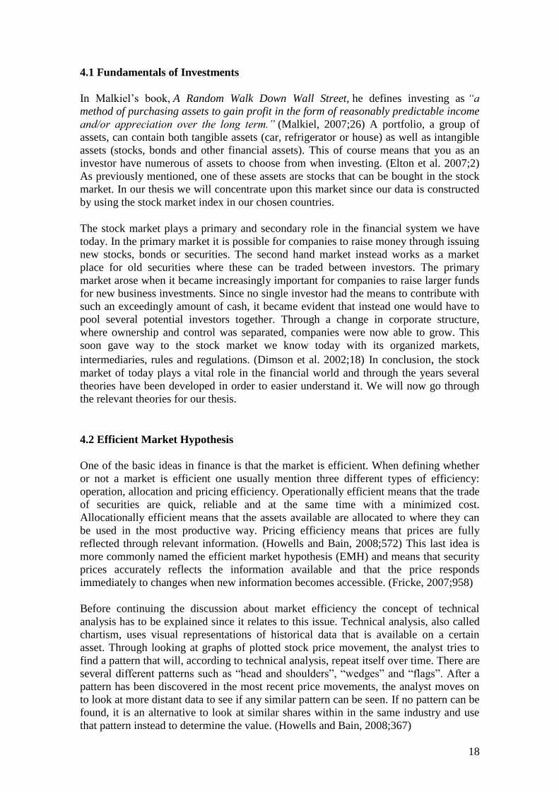
4.1 Fundamentals of Investments
In Malkiel’s book, A Random Walk Down Wall Street, he defines investing as “a
method of purchasing assets to gain profit in the form of reasonably predictable income
and/or appreciation over the long term.” (Malkiel, 2007;26) A portfolio, a group of
assets, can contain both tangible assets (car, refrigerator or house) as well as intangible
assets (stocks, bonds and other financial assets). This of course means that you as an
investor have numerous of assets to choose from when investing. (Elton et al. 2007;2)
As previously mentioned, one of these assets are stocks that can be bought in the stock
market. In our thesis we will concentrate upon this market since our data is constructed
by using the stock market index in our chosen countries.
The stock market plays a primary and secondary role in the financial system we have
today. In the primary market it is possible for companies to raise money through issuing
new stocks, bonds or securities. The second hand market instead works as a market
place for old securities where these can be traded between investors. The primary
market arose when it became increasingly important for companies to raise larger funds
for new business investments. Since no single investor had the means to contribute with
such an exceedingly amount of cash, it became evident that instead one would have to
pool several potential investors together. Through a change in corporate structure,
where ownership and control was separated, companies were now able to grow. This
soon gave way to the stock market we know today with its organized markets,
intermediaries, rules and regulations. (Dimson et al. 2002;18) In conclusion, the stock
market of today plays a vital role in the financial world and through the years several
theories have been developed in order to easier understand it. We will now go through
the relevant theories for our thesis.
4.2 Efficient Market Hypothesis
One of the basic ideas in finance is that the market is efficient. When defining whether
or not a market is efficient one usually mention three different types of efficiency:
operation, allocation and pricing efficiency. Operationally efficient means that the trade
of securities are quick, reliable and at the same time with a minimized cost.
Allocationally efficient means that the assets available are allocated to where they can
be used in the most productive way. Pricing efficiency means that prices are fully
reflected through relevant information. (Howells and Bain, 2008;572) This last idea is
more commonly named the efficient market hypothesis (EMH) and means that security
prices accurately reflects the information available and that the price responds
immediately to changes when new information becomes accessible. (Fricke, 2007;958)
Before continuing the discussion about market efficiency the concept of technical
analysis has to be explained since it relates to this issue. Technical analysis, also called
chartism, uses visual representations of historical data that is available on a certain
asset. Through looking at graphs of plotted stock price movement, the analyst tries to
find a pattern that will, according to technical analysis, repeat itself over time. There are
several different patterns such as “head and shoulders”, “wedges” and “flags”. After a
pattern has been discovered in the most recent price movements, the analyst moves on
to look at more distant data to see if any similar pattern can be seen. If no pattern can be
found, it is an alternative to look at similar shares within in the same industry and use
that pattern instead to determine the value. (Howells and Bain, 2008;367)
19
The technique is most commonly used by practitioners on the speculative market and
besides the use of chart analysis there is also cycle analysis and computerized technical
trading systems. There is however a strong criticism towards this technique, especially
in the world of academics. This can be linked to the acceptance of the efficient market
hypothesis and there has also been negative empirical findings concerning studies of
technical analysis. (Cheol-Ho, 2007;787) Below we will continue the discussion of
technical analysis in relation to market efficiency.
In 1970, Fama wrote in his article, Efficient Capital Markets, that when looking at the
market to determine whether or not it is efficient, and to what degree, there are three
different tests one can perform: weak, semi-strong and strong form test. The weak form
test use only the historical data available to determine if the price on the market reflects
the information provided (technical analysis). The semi-strong, on the other hand, also
includes publicly available information (annual earnings, press releases and the stock
price), also called fundamental analysis. The final stage is strong form, where one looks
not only on the historical data and publically available data but also include private
information that only insiders have. (Fama, 1970;383) This means that if the market is
said to be weak form, one cannot use technical analysis to outperform the market. If the
market is semi-strong, neither technical nor fundamental analysis can be used. Finally if
the market is strong form, there is no possibility, even if you have insider information,
to outperform the market since that information is already fully reflected in the price
you can find in the market. In 1991 Fama revised his earlier statements by changing
these three categories. He proposed that weak form should instead be called test for
return predictability, which include not only historical data but also forecasting returns
on dividends and yields. The other two categories, he suggested only a change in name.
From semi-strong form test to event studies and from strong form test to test for private
information. (Fama, 1991; 1576-1577)
There are some conditions that need to be met in order for the capital market to be
efficient. First of all, there should be no transaction costs, the information provided to
investors should be costless and all of market participants should agree on the
implications that the information can have on the current price of securities on the
market. If such a market exists, then we can say that it is efficient. However, this kind of
market might seem impossible to achieve and in practice, all of these conditions
actually do not need to be achieved. The requirements are sufficient for a market to be
efficient, but not necessary. This means that, for example, as long as the transactor takes
into account all of the information available, the very existence of large transaction
costs does not mean that the price does not fully reflect the available information. Also,
a market can be efficient if a large enough number of investors have access to
information about the market. It can also be seen that even though there might be
disagreement between the investors on how the market is affected by new information,
this in itself does not have to mean that the market is inefficient. With the exception that
there might be investors who repeatedly are able to make better evaluations of the
available information then what the market price imply. Then the market is said to be
inefficient. (Fama, 1970;387-388)
However, the efficient market hypothesis and its requirements have been criticized since
it seems highly unlikely that a market might meet all of these requirements. For
example there are studies that show that it is in fact necessary, not only sufficient, that
prices are costless in order for the market to be efficient. In Grossman and Stiglitz’s
(1980) research they concluded that the only way an informed investor can earn a return
on the price of collecting information is if he can use the information to reach a better
20
position in the market than an uninformed investor. However, if you believe in efficient
markets, then you know that the prices always fully reflect the information provided and
therefore it is impossible for the informed investor to earn return on his information.
(Grossman and Stiglitz, 1980;404) Over the years there have also been other studies that
have found significant anomalies when empirical testing has been conducted on the
efficient market hypothesis. (Fricke, 2007;958)
The fundamental implication of the efficient market hypothesis is that if the market is
efficient, this means that it is impossible to earn excess returns over a longer period of
time. This gives way for a process called fair game model when determining the price of
a security. If there is no relationship between what the investor estimates that the
deviation from required rate of return will be compared to the actual deviation from the
required rate of return, then the price of the security is determined by a fair game model.
A restricted form of the fair game model is the random walk model. In this model it is
said that since the past information already is calculated in the market price, then the
only thing that can change the price is news. Since news can be both good and bad, they
are said to be unpredictable. Therefore when the price reacts to news it forms a random
pattern, meaning that each return is independent of any other previous return. (Howells
and Bain, 2008;575)
4.3 Risk and Return
A central concept in financial theory is risk and return. Sharpe (1995) means that the
uncertainty about an individual security’s future price and about the future market value
of a portfolio is the primary source of risk. Furthermore, some assets and portfolios are
more risky than others. By the same reasoning, the riskiness of a portfolio is related to
the riskiness of the assets it contains. Risk is measured by the standard deviation i.e.
how much the returns vary around the average return. (Sharpe, 1995;84-88) The main
purpose with investing is to get something in return for the postponed consumption
(time value of money) and for worrying (risk of an asset). This means that investors
seek to maximize the return from an investment, given the level of risk they are willing
to accept. The return is measured by the change in the value of a portfolio. Risk-return
tradeoff is a concept explaining the relationship between the two variables discussed so
far. The principle with this concept is that return rises with risk. High uncertainty is
related to high return whereas low uncertainty is related to lower return. Investments
can give high returns if they are exposed to the risk of being lost. (Fricke, 2007;273)
21
4.4 Diversification
“Diversification is the balancing act in which the tradeoffs between risk and return are
adjusted in the light of the client’s risk tolerance.” (Bank Investment Consultant,
2006;37)
Earlier we described an investor’s portfolio as a group of assets (both tangible and
intangible) and in this section we will concentrate on how it is possible to reduce the
risk associated with these assets. Diversification can be described as a way to reduce
portfolio risk through combining assets with expected return that are less than perfectly
correlated (Fabozzi, 2010;247). Maybe an even easier way to explain it is to refer to the
adage “don’t put all of your eggs in the same basket”. The Modern Portfolio Theory
(MPT), developed by Harry Markowitz, states that through investing in more than one
asset it will be possible for the investor to diversify and thereby reducing the volatility
of the entire portfolio (Markowitz, 1959). There are different kinds of assets (stocks,
bonds and mutual funds) that an investor can hold in order to diversify a portfolio and it
is also possible that the portfolio includes assets from other classes, such as real estate
or derivatives. When the correlation of the portfolios assets is low, the portfolio will be
more diversified. When the portfolio is more diversified, standard deviation of risk will
be lower. (Bank Investment Consultant, 2006;36-37) We will describe this in more
detail later.
According to Markowitz, a good portfolio is a balanced whole that gives the investor
protection and opportunities and satisfies the needs the investor has. To be able to
distinguish which assets that should be used it is possible to look at historical data of the
asset and the expected future performance of the asset. (Markowitz, 1959;3) As
previously mentioned, an investor has to find the portfolio that offers the best risk and
return trade-off depending on his risk aversion and his need for return. This trade-off
can be seen in the efficient frontier which visualizes the relationship between risk and
return. In order for a portfolio to be efficient the portfolio must, for a given level of risk,
maximize its return. If these requirements are met, then it will lie on the efficient
frontier (Manganelli, 2003;69-70)
Figure 2 Efficient Frontier
(Maganelli, 2003;69)
22
The principle of diversification is to reduce risk and if we find assets with uncorrelated
returns we could, in theory, completely eliminate portfolio risk. However, since assets
react to same influences (business cycles and interest rates) they are correlated to some
degree and the total portfolio risk cannot be taken away entirely. (Fabozzi, 2010;247)
Wayne and Wagner (1971) demonstrated the limited risk reduction by measuring the
standard deviations of randomly selected portfolios including several assets from the
New York Stock Exchange. Their findings showed that the standard deviation declines
as the number of assets in a portfolio increases, approximately 40% of the risk of an
individual asset can be eliminated by forming randomly selected portfolios of twenty
stocks. Furthermore, their study showed that:
Total portfolio risk rapidly declines when a portfolio is expanded from one to
ten assets
The gains from diversification tend to be smaller when the portfolio consists of
more than ten assets
The return of a diversified portfolio follows the market closely
The third finding was based on the fact that the portfolio of twenty stocks had a
correlation with the market ranging between 0.8 and 0.9. This indicates that some risk
remains after diversification and was considered as a reflection of the uncertainty of the
market in general. The conclusion was that all risk cannot be eliminated. (Wayne and
Wagner, 1971;48-53)
Previously we mentioned the concept of risk and with Wayne and Wagner’s (1971)
findings in mind we have to discuss this further. The implication is that the total risk of
an asset can be divided in two categories; systematic (market, economy-wide) and
unsystematic risk (unique, idiosyncratic.) The first type of risk mentioned can, for
instance, be caused by inflation, interest rates, recessions and wars and affects a broad
range of securities. On the other hand, the second type of risk is linked only to specific
assets (Cechetti, 2008;132). See picture below.
Figure 3 Systematic and Unsystematic Risk
(Fabozzi, 2010;248)
23
The figure above illustrates that systematic and unsystematic equals the total risk of an
asset. The Y-axis represents the standard deviation of the portfolio and the X-axis
represents the number of holdings (assets). Figure A shows that unsystematic risk can
be reduced by using a diversification strategy i.e. by holding more than one asset. In
figure B the systematic risk is illustrated as a constant thus it cannot be eliminated. The
implication of this concept is that the whole risk of an asset cannot be diversified away,
only the asset unique risks can, which is in line with Wayne and Wagner’s findings.
(Fabozzi, 2010;248)
4.5 Correlation and Diversification
How related the markets i.e. returns of securities are, can be measured by using the
concept of correlation. The measures are useful for investors wanting to have a
diversified portfolio, which will be discussed later on. The most common way to
describe correlation is to use the measures +1, 0 and -1 (Sharpe, 2000;37-38). The
picture below depicts these relationships where R denotes the coefficient of correlation.
Figure 4 Correlation
(Sharpe, 2000;38)
Figure A shows the extreme case of a perfect positive relationship +1, meaning that a
movement in one market will be matched with an equal movement in another market.
Figure B depicts the other extreme, a perfect negative correlation -1. In the same
manner, if one market moves the other market also moves but in this case the movement
will be in the opposite direction. Figure C is an illustration of no correlation. A
movement in one market will have no effect on the movements in the other market, 0.
(Sharpe, 2000;38) The author Gehm (2010) claims that market correlations are almost
never negative, perfect or close to being perfect. He means that what is also important is
the stability of the correlation. If the correlation is -0.4 one year and -0.4 the next year,
it is fairly stable and diversification work reasonably well. (Gehm, 2010;53)
24
As mentioned the correlation coefficients of +1, 0 and -1 are extremes and there is a
range in between them. Ratner (2009), states that the accepted guidelines for the range
are as follows:
Values between 0 and 0.3 indicate a weak positive (negative) correlation
Values between 0.3 and 0.7 indicate a moderate positive (negative) linear
relationship
Values between 0.7 and 1.0 indicate a strong positive (negative) linear
relationship
The author claims that even though the coefficient of correlation is old, over a hundred
years, it is still going strong. However, he means that the weaknesses and the misuse of
the measure have not been studied to a greater extent and he suggests an adjusted
coefficient of correlation. (Ratner, 2009;139-142) We are aware of these new
implications but due to their limitations we will not consider them any further.
Previously we mentioned that correlation should be stable in order to gain from
diversification. However, Malkiel (2007), means that diversifying when there is a high
correlation will not help much. This means that if you invest in two markets for
diversification purposes you will not gain from this action since they move together.
The risk reduction possible from diversification when correlation exists can be
explained as follows:
Correlation Coefficient Effect of Diversification on Risk
1 no risk reduction is possible
0.5 moderate risk reduction is possible
0 considerable risk reduction is possible
-0.5 most risk can be eliminated
-1 all risk can be eliminated
The reasoning behind this comes from one of Markowitz contributions concerning risk
reduction. Luckily, for investors, risk reduction from diversification is possible even
though the correlation is not negative. Determining whether adding an asset will reduce
risk or not is the crucial role of the coefficient correlation and it has been demonstrated
above. This means that with a correlation that is anything less than perfectly linear, a
portfolio’s risk can be reduced. (Malkiel, 2007;190) In conclusion, the lesser correlation
the better the effect from diversification will be. It should be noted that this is true no
matter how risky the securities are in isolation (Fabozzi, 2010;247).
4.6 International Diversification
In the previous section we have concluded that a diversified portfolio containing several
assets will carry less risk than the separate parts alone. Odier and Solnik (1993), Solnik
(1995) and Ming-Yuan (2007), have all studied the benefits from international
diversification. Their results show that by investing internationally it is possible to both
reduce risk and increase profit opportunities. Furthermore, an international portfolio
makes it possible to expand the efficient frontier and reduce the systematic risk level
below that of domestic securities alone. The reasoning behind international investments
is that structural and cyclical differences across economies makes the risk-reduction
25
benefit possible. If one market is doing worse than expected it is likely that another
market will do better than the expectations, hence the risk is reduced and losses are
offset. The authors conclude that international assets are an important component of
asset allocation for an investor since the risk and return advantages are very large in all
major countries. (Odier and Solnik, 1993, Solnik, 1995, Ming-Yuan, 2007)
Odier and Solnik (1993) discussed whether these benefits would continue in the future
and argued that it depends on cross-country correlations and market volatilities. They
stated that there was little evidence of increased volatility in the world markets and that
correlation between the markets remains fairly low, which is positive for international
investments. This development was supported by Ming-Yuan (2007). The negative side
is that the correlation tends to increase during volatile periods, when the diversification
offered from low correlation is most needed. (Odier and Solnik, 1993;89) In 1996
Karolyi and Stulz also found evidence for high correlation when markets move a lot.
(Karolyi and Stulz, 1996) Later, this has once again been proven to be true. In their
article, Does Correlation Between Stock Market Returns Really Increase During
Turbulent Periods? Chesney and Jondeau (2001) investigated the relationship between
international correlation and stock market turbulence. Their findings showed that the
markets are more highly correlated during high-volatile periods than during low-
volatility periods. (Chesney and Jondeau, 2001;74) This finding is important for
investors since the benefits from diversification seem to decrease during volatile periods
when they are most needed. In order to form an optimal portfolio it is important to
determine the correlation between the assets, but if the correlation increases when the
market is turbulent the standard portfolio diversification cannot reduce the risk during
these periods. Therefore the key to good asset allocation is somewhat harder to use.
(Chesney and Jondeau, 2001;53)
To conclude this chapter we can say that the stock market plays a vital role in the
financial system today and there are many theories connected to this. Most of them lie
on the assumption that the market is, to some degree, efficient. Risk and return are
central concepts and taking on risk is necessary in order to increase capital gains.
However, it is not necessary to carry all risk, the so called unsystematic risk can be
diversified away by investing in several assets and on different markets. Correlation
between different stock markets can make diversification more complicated and is
therefore important to study.
26
5. Data Collection
In this chapter we will mainly present in which ways we gathered the data used in our study. The database, DataStream will be discussed as well the method used to access the necessary data. The reader will be given a knowledge base about stock indexes and we will also briefly present the chosen indexes. Furthermore we will discuss the criteria of a research.
The purpose of the chapter is to give the reader a greater understanding of the practical aspects of our study.
"All you can do is the best you can do."
- Paula Abdul
27
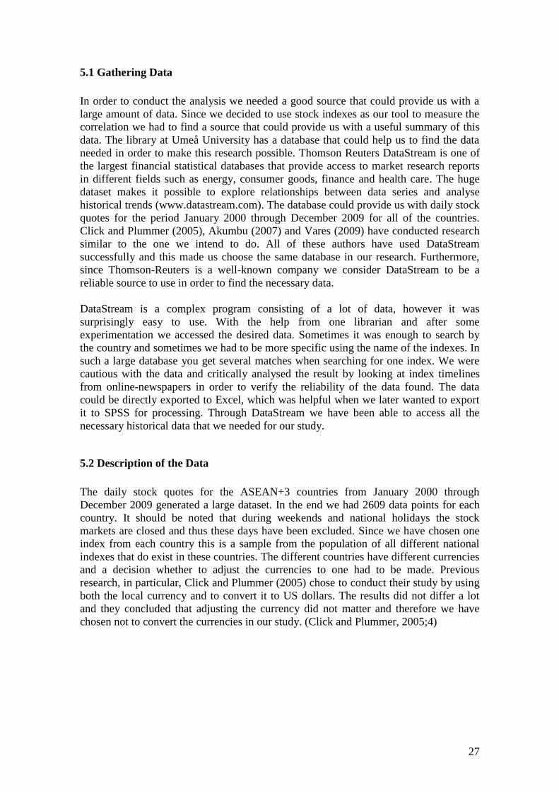
5.1 Gathering Data
In order to conduct the analysis we needed a good source that could provide us with a
large amount of data. Since we decided to use stock indexes as our tool to measure the
correlation we had to find a source that could provide us with a useful summary of this
data. The library at Umeå University has a database that could help us to find the data
needed in order to make this research possible. Thomson Reuters DataStream is one of
the largest financial statistical databases that provide access to market research reports
in different fields such as energy, consumer goods, finance and health care. The huge
dataset makes it possible to explore relationships between data series and analyse
historical trends (www.datastream.com). The database could provide us with daily stock
quotes for the period January 2000 through December 2009 for all of the countries.
Click and Plummer (2005), Akumbu (2007) and Vares (2009) have conducted research
similar to the one we intend to do. All of these authors have used DataStream
successfully and this made us choose the same database in our research. Furthermore,
since Thomson-Reuters is a well-known company we consider DataStream to be a
reliable source to use in order to find the necessary data.
DataStream is a complex program consisting of a lot of data, however it was
surprisingly easy to use. With the help from one librarian and after some
experimentation we accessed the desired data. Sometimes it was enough to search by
the country and sometimes we had to be more specific using the name of the indexes. In
such a large database you get several matches when searching for one index. We were
cautious with the data and critically analysed the result by looking at index timelines
from online-newspapers in order to verify the reliability of the data found. The data
could be directly exported to Excel, which was helpful when we later wanted to export
it to SPSS for processing. Through DataStream we have been able to access all the
necessary historical data that we needed for our study.
5.2 Description of the Data
The daily stock quotes for the ASEAN+3 countries from January 2000 through
December 2009 generated a large dataset. In the end we had 2609 data points for each
country. It should be noted that during weekends and national holidays the stock
markets are closed and thus these days have been excluded. Since we have chosen one
index from each country this is a sample from the population of all different national
indexes that do exist in these countries. The different countries have different currencies
and a decision whether to adjust the currencies to one had to be made. Previous
research, in particular, Click and Plummer (2005) chose to conduct their study by using
both the local currency and to convert it to US dollars. The results did not differ a lot
and they concluded that adjusting the currency did not matter and therefore we have
chosen not to convert the currencies in our study. (Click and Plummer, 2005;4)
When conducting a study it is important to discuss some research criteria; reliability,
validity, generalsability and replication. We will begin our discussion with the
reliability of the research. The intention with this measure is to evaluate if the results of
the study would be the same if it was conducted by someone else, meaning if it is
reliable or not (Halvorsen (1992;46). Bryman and Bell (2007) discusses reliability in
terms of: stability, internal reliability and inter-observer consistency (2007;149).
The stability concerns whether the observations and results are stable over time we
believe that it can be evaluated by using these three questions:
1. Will similar observations be obtained by other researchers?
2. Will the measure yield the same results on another occasion?
3. Is there a clear transparency on how data have been used to draw the relevant
conclusions?
(Easterby-Smith et. al. 2002;53)
As mentioned before, the database DataStream, which we have been using in this
research is reliable. Based on this reasoning we believe that other researchers would
obtain similar observations as we did. The data is raw data, meaning that it is free from
interpretations and the default risk for DataStream must be considered to be low. The
datapoints for the stock market indexes are history and fixed for each day and therefore
the observations will not change. If someone was to conduct the same research as we
have done the probability that the results would be the same is high. Of course we may
have plotted the data wrong, which would lead to another result, however the difference
would not be significant since the data contains a high reliability. We have tried to make
the use of the data transparent to the reader in order to make the study more reliable. In
our data collection chapter we present the data thoroughly so that the reader can
understand how we have reached our conclusions.
If the measures used for obtaining the findings are applicable to the research question is
the meaning of internal reliability (Bryman and Bell, 2007;150). The main measure
used is correlation and this must be considered to be in line with our research questions
since our intention is to measure correlation. There are many different ways in which
correlation can be measured and the choice to use Pearson correlation was based on our
statistical knowledge and since it is applicable to the research questions it must be
considered reasonable.
Inter-observer consistency relates to the subjectivism of the research. The measures may
not be consistent with the results if the researcher has made personal interpretations
(Bryman and Bell 2007; 150). As previously discussed we have been aiming for an
objective perspective and the data used have not given us any opportunity to make any
judgments or interpretations. The data and the measure must be considered to be
consistent with our conclusions.
32
5.5 Validity
Validity refers to that the data collected and used must be relevant and good enough for
interpretation of the final results (Bryman and Bell, 2007; 151). Johansson Lindfors
(1993) argues that when the researcher uses data that has been collected by someone
else for example a database it can be difficult to get information about the
representativeness of the data. This would in turn affect the validity of the study.
(Johansson Lindfors, 1993;118) We have previously discussed DataStream as a reliable
source. It is one of the largest financial databases and the risk of inference with the
objectivity of the data is small. The data has not been analysed by anyone, and in our
opinion, this adds validity to the data as well as the results.
5.6 Generalisability
The transferability of a study is already decided when the researcher collects the sample.
To investigate the whole population is rarely possible and a sample has to be made. The
question is then how representative the sample is of the population i.e. if a research
including the whole population would generate the same results (Johansson Lindfors,
1993;162). In our study we have made some limitations to how many indexes to include
and we also consider the chosen indexes to be our sample. The sample is very large with
high significance and can be used for generalization purposes. Johansson Lindfors
(1993) means that even if you conduct a large sample or study the whole population the
generalisability of a model cannot be certain. There is a risk that random errors occur
and this would cause bias in the collection of the data. (Johansson Lindfors 1993;162)
Of course, this is something that may have occurred in our study, when collecting the
data and transferring it to SPSS some errors can always occur. Even if we cannot
guarantee that the study is free from bias we still argue that the errors should not be seen
as extensive and hence it has no significant influence on the result. The conclusion,
based on the large sample, is that the results can be generalised and a similar result
would have been obtained if investigating the population of all national stock indexes
for the countries.
5.7 Replication
The criterion replication is important when there are researchers that want to repeat your
study, in order to make a study replicable it is important to state the process in detail.
For example what methods you have used, how the data was collected and processed
must be clearly stated. (Bryman and Bell, 2007;171). Once again, in our data collection
chapter, we give the reader a thorough explanation of the indexes, the database and how
we have processed the data. Furthermore, by describing our preconceptions, perspective
and approach we have given other researchers the possibility to repeat our study from
the same standpoint.
33
6. Empirical Findings
Chapter six will state the empirical findings of our research. We have divided the chapter in to two parts. First we will present the results for the whole period for each country. Secondly, we will present the yearly correlation in more detail.
The purpose of the chapter is to give the reader an overview of the result from our
statistical analysis of the data.
“However beautiful the strategy, you should occasionally look at the results.”
- Sir Winston Churchill
34
6.1 Correlation by Country
In this section we will present our empirical findings of the correlation from 2000 until
2009. Beginning with all of the countries and then continuing country by country.
When conducting Pearson correlation for the whole time period we had a statistically
significant result. Correlation is significant at the 0.01 level in a two tail test and all of
our data had a value lower than 0.01 meaning that it was significant. (Appendix 1) In
our theoretical framework we discussed the different ranges of correlation that we will
use when presenting our findings. Below they are shown once again;
Values between 0 and 0.3 indicate a weak positive (negative) correlation
Values between 0.3 and 0.7 indicate a moderate positive (negative) linear
relationship
Values between 0.7 and 1.0 indicate a strong positive (negative) linear
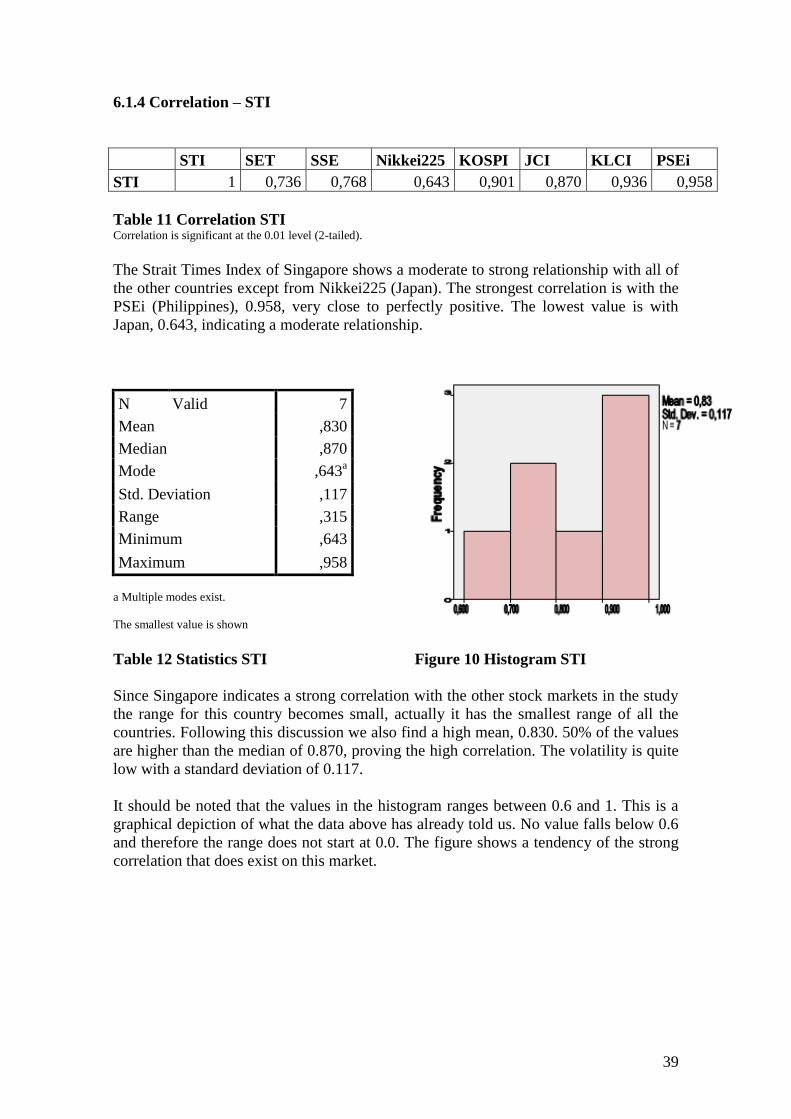
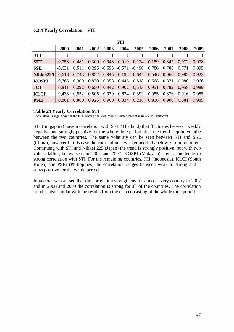
relationship6.1.1 Correlation ASEAN+3
JCI KLCI PSEi STI SET SSE Nikkei225 KOSPI
JCI 1 0,942 0,938 0,870 0,771 0,764 0,247 0,964
KLCI 1 0,956 0,936 0,779 0,782 0,436 0,937
PSEi 1 0,958 0,760 0,779 0,489 0,941
STI 1 0,736 0,768 0,643 0,901
SET 1 0,413 0,291 0,807
SSE 1 0,305 0,721
Nikkei225 1 0,369
KOSPI 1
Table 3 Correlation ASEAN+3 Correlation is significant at the 0.01 level (2-tailed).
After looking at Table 3 we can see that the overall correlation seems to be relatively
high, meaning that many values are close to 1.0.
The data output ranges between weak to strong.
It can also be concluded that we have no zero,
perfectly negative or positive correlation. The
strongest correlation we found was between
KOSPI (South Korea) and JCI (Indonesia) which
had a value of 0.964, the closest to perfectly
positive linear relationship. On the other hand we
also have Nikkei 225 (Japan) and JCI with a
correlation of only 0.247, a result which shows
weak correlation. From Table 4 it can also be
found that the mean value was 0.722, which
indicates a strong positive linear relationship on Table 4 Statistics ASEAN+3
average. The value 0.779 occurs twice, i.e. the mode.
The median value shows a strong correlation with 50% of the values above 0.775. Even
though 50% lies below 0.775, it can still be concluded, by looking at Table 3, that the
correlation is moderate, except for one value (0.247). In our descriptive statistics we
have also included the standard deviation, which explains that 68% of the observed
N Valid 28
Mean ,722
Median ,775
Mode ,779
Std. Deviation ,230
Range ,717
Minimum ,247
Maximum ,964
35
value lies + or – 0.230 from the mean 0.722. The implication is that the volatility is
moderate in our data resulting in an overall high correlation.
The relationships explained
above are graphically depicted
in the histogram to the right.
From the graph it is possible
to see that the four bars to the
right have a higher frequency
than the three bars to the left.
Once again, this is an
indication of an overall strong
positive correlation.
Figure 5 Histogram ASEAN+3
In Figure 6 the stock indexes are matched against each other to give the reader a
graphical overview of the development. For instance looking at KOSPI and JCI, that
have a correlation of 0.964, it is possible to see that they follow each other in the graph.
On the other hand it is also possible to see that Nikkei and JCI, with a low correlation of
0.247, do not follow each other. Hence, the times series are in line with what we
previously observed in Pearson correlation.
Figure 6 Line Chart ASEAN+31
1 Since we have used the local currency, we had to factor down the Japanese yen in order to get a
smoother graph. This had no effect on the correlation.
0
1000
2000
3000
4000
5000
6000
7000
1-3
-2000
7-3
-2000
1-3
-2001
7-3
-2001
1-3
-2002
7-3
-2002
1-3
-2003
7-3
-2003
1-3
-2004
7-3
-2004
1-3
-2005
7-3
-2005
1-3
-2006
7-3
-2006
1-3
-2007
7-3
-2007
1-3
-2008
7-3
-2008
1-3
-2009
7-3
-2009
Lo
cal
cu
rren
cy
Date
INDEX ASEAN+3
JCI
KLCI
PSEi
STI
SET
SSE
Nikkei225
KOSPI
36
6.1.1 Correlation – JCI
Table 5 Correlation JCI Correlation is significant at the 0.01 level (2-tailed).
When looking at the Jakarta Composite Index in Indonesia it is clear that the correlation
is high, above 0.7, with all of the countries except for Nikkei225 (Japan). As we
previously mentioned, Indonesia, is the country that has the highest and lowest
correlation values.
Table 6 Statistics JCI Figure 7 Histogram JCI
Since Indonesia has the highest and lowest correlation values, it also has the same
range, 0.717, as the overall data output. Following the strong correlation it can be
expected that the mean and median are high. The mean is 0.785 slightly higher than for
the data with all of the countries (see table 4, 0.772). Looking at the median it is also
higher with 50% of the values being above 0.870, compared to 0.775 for the whole
dataset. The standard deviation is quite similar to the overall data, thus moderately
volatile with a value of 0.251.
In Figure 7 the histogram shows the division of the values. It is clear that the correlation
is closer to 1.0 than 0.0.
JCI KLCI PSEi STI SET SSE Nikkei225 KOSPI
JCI 1 0,942 0,938 0,870 0,771 0,764 0,247 0,964
N Valid 7
Mean ,785
Median ,870
Mode ,247a
Std. Deviation ,251
Range ,717
Minimum ,247
Maximum ,964
a. Multiple modes exist. The smallest value is
shown
37
6.1.2 Correlation – KLCI
KLCI PSEi STI SET SSE Nikkei225 KOSPI JCI
KLCI 1 0,956 0,936 0,779 0,782 0,436 0,937 0,942
Table 7 Correlation KLCI Correlation is significant at the 0.01 level (2-tailed).
Kuala Lumpur Composite Index representing Malaysia’s stock market have four values
above 0.9, two around 0.8 and one below 0.5. This means that Malaysia has a strong
correlation with six of the other countries and a moderate positive linear relationship
with Nikkei225 (Japan).
N Valid 7
Mean ,824
Median ,936
Mode ,436a
Std. Deviation ,188
Range ,520
Minimum ,436
Maximum ,956
a. Multiple modes exist. The smallest value is
shown
Table 8 Statistics KLCI Figure 8 Histogram KLCI
The range for Malaysia is 0.520 which is lower than the range for the whole dataset
(0.717). Since most of the countries have a strong correlation with Malaysia the mean
also has a high value, 0.824. It can be noted that the median of 0.936 is significantly
higher for Malaysia in comparison to the median found in the data over all countries
(0.775). Once again the data has proven that high correlation exists between Malaysia
and the other countries. The standard deviation of 0.188 indicates that the values are less
volatile than in the previous case of Indonesia.
As previously mentioned the correlation for Malaysia is strong and moderate positive
linear, and this can be seen in the histogram for KLCI. The bar to the left represents the
moderate relationship and the two bars to the right represent the strong relationship.
38
6.1.3 Correlation – PSEi
PSEi STI SET SSE Nikkei225 KOSPI JCI KLCI
PSEi 1 0,958 0,760 0,779 0,489 0,941 0,938 0,956
Table 9 Correlation PSEi Correlation is significant at the 0.01 level (2-tailed).
The Philippines Stock Exchange index shows a correlation that is higher than 0.3 for all
of the countries which indicates a moderate or strong correlation. It is only Nikkei 225
(Japan) that has only a moderate correlation with PSEi (0.489). Both KOSPI (South
Korea), JCI (Indonesia), KLCI (Malaysia and STI (Singapore) has a correlation of over
0.9 which is an almost perfect positive linear relationship with PSEi.
N Valid 7
Mean ,832
Median ,938
Mode ,489a
Std. Deviation ,173
Range ,469
Minimum ,489
Maximum ,958
a. Multiple modes exist. The smallest value is
shown
Table 10 Statistics PSEi Figure 9 Histogram PSEi
Since PSEi has a very high correlation with all but Japan the mean, 0.832, is high. Also
because most of the correlations lie above 0.9 the median is as high as 0.938, compared
to the data for all of the countries that is 0.775. This indicates that PSEi has a very
strong correlation with the other countries. The range is 0.469, which means that all of
the values lie closer together than the data for all of the countries and also the standard
deviation is only 0.172, meaning that 68% of the correlation values are + or – 0.173
from the mean. This can also be seen in the histogram since most of the observed data is
close to 0.8.
The histogram shows that even though there are some observed data with less
correlation, most of the data is higher than 0.9 and the rest is still higher than 0.3, which
means there is a moderate or strong relationship
39
6.1.4 Correlation – STI
STI SET SSE Nikkei225 KOSPI JCI KLCI PSEi
STI 1 0,736 0,768 0,643 0,901 0,870 0,936 0,958
Table 11 Correlation STI Correlation is significant at the 0.01 level (2-tailed).
The Strait Times Index of Singapore shows a moderate to strong relationship with all of
the other countries except from Nikkei225 (Japan). The strongest correlation is with the
PSEi (Philippines), 0.958, very close to perfectly positive. The lowest value is with
Japan, 0.643, indicating a moderate relationship.
N Valid 7
Mean ,830
Median ,870
Mode ,643a
Std. Deviation ,117
Range ,315
Minimum ,643
Maximum ,958
a Multiple modes exist.
The smallest value is shown
Table 12 Statistics STI Figure 10 Histogram STI
Since Singapore indicates a strong correlation with the other stock markets in the study
the range for this country becomes small, actually it has the smallest range of all the
countries. Following this discussion we also find a high mean, 0.830. 50% of the values
are higher than the median of 0.870, proving the high correlation. The volatility is quite
low with a standard deviation of 0.117.
It should be noted that the values in the histogram ranges between 0.6 and 1. This is a
graphical depiction of what the data above has already told us. No value falls below 0.6
and therefore the range does not start at 0.0. The figure shows a tendency of the strong
correlation that does exist on this market.
40
6.1.5 Correlation – SET
Table 13 Correlation SET Correlation is significant at the 0.01 level (2-tailed).
Looking at SET, Thailand’s Stock Exchange, one can see that correlation with Nikkei
225 (Japan) is only 0.291, which is lower than 0.3 and indicates a weak positive
relationship. The correlation between SET and SSE (China) is only moderately positive
in comparison with STI (Singapore), KLCI (Malaysia), PSEi (Philippine) and KOSPI
(South Korea) were the correlation is above 0.7, meaning that the correlation is strong.
N Valid 7
Mean ,651
Median ,760
Mode ,291a
Std. Deviation ,208
Range ,516
Minimum ,291
Maximum ,807
a. Multiple modes exist. The smallest value is
shown
Table 14 Statistics SET Figure 11 Histogram SET
Compared to the data for all of the countries, SET shows a quite low mean of 0.651.
The minimum observed correlation is 0.291 and the maximum is 0.807, giving us a
range of 0.516. The standard deviation is 0.208, which indicates a slightly lower
volatility than for the data set of all the countries (0.230). The median is 0.760 which
means that 50% of the values lie above this and is therefore considered to have a strong
positive linear relationship.
The histogram graphical shows us that most of the correlations lie below 0.8. However,
most of the correlations are still above 0.3, indicating a stronger positive relationship. It
is also shown that a larger part of the observed correlations are between 0.7 and 0.8.
SET SSE Nikkei225 KOSPI JCI KLCI PSEi STI
SET 1 0,413 0,291 0,807 0,771 0,779 0,760 0,736
41
6.1.6 Correlation – SSE
SSE Nikkei225 KOSPI JCI KLCI PSEi STI SET
SSE 1 0,305 0,721 0,764 0,782 0,779 0,768 0,413
Table 15 Correlation SSE Correlation is significant at the 0.01 level (2-tailed).
China’s Shanghai Stock Exchange index has a correlation that is higher than 0.3 with all
of the countries, meaning that all of them have either a moderate or strong positive
linear relationship. Nikkei 225 (Japan) and SET (Thailand) has a moderately positive
linear relationship with SSE with values of 0.305 and 0.413 respectively. All of the
other countries show values of above 0.7 and therefore indicates strong positive
correlation.
N Valid 7
Mean ,647
Median ,764
Mode ,305a
Std. Deviation ,200
Range ,477
Minimum ,305
Maximum ,782
a. Multiple modes exist. The smallest
value is shown
Table 16 Statistics SSE Figure 12 Histogram SSE
It can be seen that there is a very strong similarity between SSE and SET. SSE has a
mean (0.647) and median (0.764) that is close to the values we previously saw in the
presentation of SET (0.651 and 0.760 respectively). The standard deviation is also close
to each other with SSE having a standard deviation of 0.200 and SET with 0.208. There
is a small difference in the range since SSE has a minimum value of 0.305 and
maximum value of 0.782, giving the data a range of 0.477 compared to SET with a
range of 0.516. Even though their numbers are quite a like, the histogram still shows a
small difference. SSE, for example, does not have any observed values above 0.8 and
none below 0.3.Then again, most of the observed values are between 0.7 and 0.8 and
there is gap between 0.5 and 0.7 where no observed values can be found. The same