Chapter 7

Diversity

In Chapter 6 we saw that both Rayleigh fading and log normal shadowing induce a very large power penalty on theperformance of modulation over wireless channels. One of the most powerful techniques to mitigate the effects offading is to use diversity-combining of independently fading signal paths. Diversity-combining uses the fact thatindependent signal paths have a low probability of experiencing deep fades simultaneously. Thus, the idea behinddiversity is to send the same data over independent fading paths. These independent paths are combined in someway such that the fading of the resultant signal is reduced. For example, consider a system with two antennasat either the transmitter or receiver that experience independent fading. If the antennas are spaced sufficientlyfar apart, it is unlikely that they both experience deep fades at the same time. By selecting the antenna withthe strongest signal, called selection combining, we obtain a much better signal than if we just had one antenna.This chapter focuses on common techniques at the transmitter and receiver to achieve diversity. Other diversitytechniques that have potential benefits over these schemes in terms of performance or complexity are discussed in[1, Chapter 9.10].

Diversity techniques that mitigate the effect of multipath fading are called microdiversity, and that is the focusof this chapter. Diversity to mitigate the effects of shadowing from buildings and objects is called macrodiversity.Macrodiversity is generally implemented by combining signals received by several base stations or access points.This requires coordination among the different base stations or access points. Such coordination is implementedas part of the networking protocols in infrastructure-based wireless networks. We will therefore defer discussionof macrodiversity until Chapter 15, where we discuss the design of such networks.

7.1 Realization of Independent Fading Paths

There are many ways of achieving independent fading paths in a wireless system. One method is to use multipletransmit or receive antennas, also called an antenna array, where the elements of the array are separated in distance.This type of diversity is referred to as space diversity. Note that with receiver space diversity, independent fadingpaths are realized without an increase in transmit signal power or bandwidth. Moreover, coherent combiningof the diversity signals leads to an increase in SNR at the receiver over the SNR that would be obtained withjust a single receive antenna, which we discuss in more detail below. Conversely, to obtain independent pathsthrough transmitter space diversity, the transmit power must be divided among multiple antennas. Thus, withcoherent combining of the transmit signals the received SNR is the same as if there were just a single transmitantenna. Space diversity also requires that the separation between antennas be such that the fading amplitudescorresponding to each antenna are approximately independent. For example, from (3.26) in Chapter 3, in a uniformscattering environment with isotropic transmit and receive antennas the minimum antenna separation required forindependent fading on each antenna is approximately one half wavelength ( .38λ to be exact). If the transmit or

190

receive antennas are directional (which is common at the base station if the system has cell sectorization), thenthe multipath is confined to a small angle relative to the LOS ray, which means that a larger antenna separation isrequired to get independent fading samples [2].

A second method of achieving diversity is by using either two transmit antennas or two receive antennas withdifferent polarization (e.g. vertically and horizontally polarized waves). The two transmitted waves follow thesame path. However, since the multiple random reflections distribute the power nearly equally relative to bothpolarizations, the average receive power corresponding to either polarized antenna is approximately the same.Since the scattering angle relative to each polarization is random, it is highly improbable that signals receivedon the two differently polarized antennas would be simultaneously in deep fades. There are two disadvantagesof polarization diversity. First, you can have at most two diversity branches, corresponding to the two types ofpolarization. The second disadvantage is that polarization diversity loses effectively half the power (3 dB) sincethe transmit or receive power is divided between the two differently polarized antennas.

Directional antennas provide angle, or directional, diversity by restricting the receive antenna beamwidth toa given angle. In the extreme, if the angle is very small then at most one of the multipath rays will fall within thereceive beamwidth, so there is no multipath fading from multiple rays. However, this diversity technique requireseither a sufficient number of directional antennas to span all possible directions of arrival or a single antenna whosedirectivity can be steered to the angle of arrival of one of the multipath components (preferably the strongest one).Note also that with this technique the SNR may decrease due to the loss of multipath components that fall outsidethe receive antenna beamwidth, unless the directional gain of the antenna is sufficiently large to compensate forthis lost power. Smart antennas are antenna arrays with adjustable phase at each antenna element: such arraysform directional antennas that can be steered to the incoming angle of the strongest multipath component [3].

Frequency diversity is achieved by transmitting the same narrowband signal at different carrier frequencies,where the carriers are separated by the coherence bandwidth of the channel. This technique requires additionaltransmit power to send the signal over multiple frequency bands. Spread spectrum techniques, discussed in Chapter13, are sometimes described as providing frequency diversity since the channel gain varies across the bandwidthof the transmitted signal. However, this is not equivalent to sending the same information signal over indepedentlyfading paths. As discussed in Chapter 13.2.4, spread spectrum with RAKE reception does provide independentlyfading paths of the information signal and thus is a form of frequency diversity. Time diversity is achieved bytransmitting the same signal at different times, where the time difference is greater than the channel coherencetime (the inverse of the channel Doppler spread). Time diversity does not require increased transmit power, but itdoes decrease the data rate since data is repeated in the diversity time slots rather than sending new data in thesetime slots. Time diversity can also be achieved through coding and interleaving, as will be discussed in Chapter8. Clearly time diversity can’t be used for stationary applications, since the channel coherence time is infinite andthus fading is highly correlated over time.

In this chapter we will focus on space diversity as a reference to describe the diversity systems and thedifferent combining techniques, although the combining techniques can be applied to any type of diversity. Thus,the combining techniques will be defined as operations on an antenna array. Receiver and transmitter diversity aretreated separately, since the system models and diversity combining techniques for each have important differences.

7.2 Receiver Diversity

7.2.1 System Model

In receiver diversity the independent fading paths associated with multiple receive antennas are combined to obtaina resultant signal that is then passed through a standard demodulator. The combining can be done in several wayswhich vary in complexity and overall performance. Most combining techniques are linear: the output of the

191

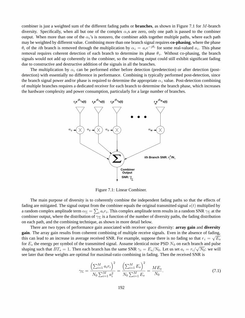
combiner is just a weighted sum of the different fading paths or branches, as shown in Figure 7.1 for M -branchdiversity. Specifically, when all but one of the complex αis are zero, only one path is passed to the combineroutput. When more than one of the αi’s is nonzero, the combiner adds together multiple paths, where each pathmay be weighted by different value. Combining more than one branch signal requires co-phasing, where the phaseθi of the ith branch is removed through the multiplication by αi = aie

−jθi for some real-valued ai. This phaseremoval requires coherent detection of each branch to determine its phase θ i. Without co-phasing, the branchsignals would not add up coherently in the combiner, so the resulting output could still exhibit significant fadingdue to constructive and destructive addition of the signals in all the branches.

The multiplication by αi can be performed either before detection (predetection) or after detection (post-detection) with essentially no difference in performance. Combining is typically performed post-detection, sincethe branch signal power and/or phase is required to determine the appropriate α i value. Post-detection combiningof multiple branches requires a dedicated receiver for each branch to determine the branch phase, which increasesthe hardware complexity and power consumption, particularly for a large number of branches.

Σ

α1 α3α2 αM

1

j θ1r e s(t)j θ

2r e s(t)23r e s(t)

j θ3 j θM

Mr e s(t)

i2ith Branch SNR: r /N i

Combiner Output

γΣ

SNR:

Figure 7.1: Linear Combiner.

The main purpose of diversity is to coherently combine the independent fading paths so that the effects offading are mitigated. The signal output from the combiner equals the original transmitted signal s(t) multiplied bya random complex amplitude term αΣ =

∑i airi. This complex amplitude term results in a random SNR γΣ at the

combiner output, where the distribution of γΣ is a function of the number of diversity paths, the fading distributionon each path, and the combining technique, as shown in more detail below.

There are two types of performance gain associated with receiver space diversity: array gain and diversitygain. The array gain results from coherent combining of multiple receive signals. Even in the absence of fading,this can lead to an increase in average received SNR. For example, suppose there is no fading so that r i =

√Es

for Es the energy per symbol of the transmitted signal. Assume identical noise PSD N0 on each branch and pulseshaping such that BTs = 1. Then each branch has the same SNR γi = Es/N0. Let us set ai = ri/

√N0: we will

see later that these weights are optimal for maximal-ratio combining in fading. Then the received SNR is

γΣ =

(∑Mi=1 airi

)2

N0∑M

i=1 a2i

=

(∑Mi=1 Es

)2

N0∑M

i=1 Es

=MEs

N0. (7.1)

192

Thus, in the absence of fading, with appropriate weighting there is an M -fold increase in SNR due to the coherentcombining of the M signals received from the different antennas. This SNR increase in the absence of fading isrefered to as the array gain. More precisely, array gain Ag is defined as the increase in averaged combined SNRγΣ over the average branch SNR γ:

Ag =γΣ

γ.

Array gain occurs for all diversity combining techniques, but is most pronounced in MRC. Both diversity andarray gain occur in transmit diversity as well. The array gain allows a system with multiple transmit or receiveantennas in a fading channel to achieve better performance than a system without diversity in an AWGN channelwith the same average SNR. We will see this effect in performance curves for MRC and EGC with a large numberof antennas.

In fading the combining of multiple independent fading paths leads to a more favorable distribution for γΣ

than would be the case with just a single path. In particular, the performance of a diversity system, whether it usesspace diversity or another form of diversity, in terms of P s and Pout is as defined in Sections AveErrorProb-6.3.1:

P s =∫ ∞

0Ps(γ)pγΣ(γ)dγ, (7.2)

where Ps(γ) is the probability of symbol error for demodulation of s(t) in AWGN with SNR γΣ, and

Pout = p(γΣ ≤ γ0) =∫ γ0

0pγΣ(γ)dγ, (7.3)

for some target SNR value γ0. The more favorable distribution for γΣ leads to a decrease in P s and Pout due todiversity combining, and the resulting performance advantage is called the diversity gain. In particular, for somediversity systems their average probability of error can be expressed in the form P s = cγ−M where c is a constantthat depends on the specific modulation and coding, γ is the average received SNR per branch, and M is calledthe diversity order of the system. The diversity order indicates how the slope of the average probability of erroras a function of average SNR changes with diversity. Figures 7.3 and 7.6 below show these slope changes as afunction of M for different combining techniques. Recall from (6.61) that a general approximation for averageerror probability in Rayleigh fading with no diversity is P s ≈ αM/(2βMγ). This expression has a diversity orderof one, consistent with a single receive antenna. The maximum diversity order of a system with M antennas is M ,and when the diversity order equals M the system is said to achieve full diversity order.

In the following subsections we will describe the different combining techniques and their performance inmore detail. These techniques entail various tradeoffs between performance and complexity.

7.2.2 Selection Combining

In selection combining (SC), the combiner outputs the signal on the branch with the highest SNR r2i /Ni. This is

equivalent to choosing the branch with the highest r2i + Ni if the noise power Ni = N is the same on all branches

1. Since only one branch is used at a time, SC often requires just one receiver that is switched into the activeantenna branch. However, a dedicated receiver on each antenna branch may be needed for systems that transmitcontinuously in order to simultaneously and continuously monitor SNR on each branch. With SC the path outputfrom the combiner has an SNR equal to the maximum SNR of all the branches. Moreover, since only one branchoutput is used, co-phasing of multiple branches is not required, so this technique can be used with either coherentor differential modulation.

1In practice r2i + Ni is easier to measure than SNR since it just entails finding the total power in the received signal.

193

For M branch diversity, the CDF of γΣ is given by

PγΣ(γ) = p(γΣ < γ) = p(max[γ1, γ2, . . . , γM ] < γ) =M∏i=1

p(γi < γ). (7.4)

We obtain the pdf of γΣ by differentiating PγΣ(γ) relative to γ, and the outage probability by evaluating PγΣ(γ)at γ = γ0. Assume that we have M branches with uncorrelated Rayleigh fading amplitudes ri. The instantaneousSNR on the ith branch is therefore given by γi = r2

i /N . Defining the average SNR on the ith branch as γ i = E[γi],the SNR distribution will be exponential:

p(γi) =1γi

e−γi/γi . (7.5)

From (6.47), the outage probability for a target γ0 on the ith branch in Rayleigh fading is

Pout(γ0) = 1 − e−γ0/γi . (7.6)

The outage probability of the selection-combiner for the target γ0 is then

Pout(γ0) =M∏i=1

p(γi < γ0) =M∏i=1

[1 − e−γ0/γi

]. (7.7)

If the average SNR for all of the branches are the same (γ i = γ for all i), then this reduces to

Pout(γ0) = p(γΣ < γ0) =[1 − e−γ0/γ

]M. (7.8)

Differentiating (7.8) relative to γ0 yields the pdf for γΣ:

pγΣ(γ) =M

γ

[1 − e−γ/γ

]M−1e−γ/γ . (7.9)

From (7.9) we see that the average SNR of the combiner output in i.i.d. Rayleigh fading is

γΣ =∫ ∞

0γpγΣ(γ)dγ

=∫ ∞

0

γM

γ

[1 − e−γ/γ

]M−1e−γ/γdγ

= γM∑i=1

1i. (7.10)

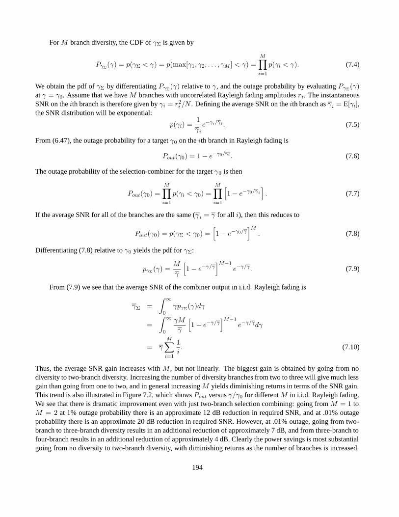
Thus, the average SNR gain increases with M , but not linearly. The biggest gain is obtained by going from nodiversity to two-branch diversity. Increasing the number of diversity branches from two to three will give much lessgain than going from one to two, and in general increasing M yields diminishing returns in terms of the SNR gain.This trend is also illustrated in Figure 7.2, which shows Pout versus γ/γ0 for different M in i.i.d. Rayleigh fading.We see that there is dramatic improvement even with just two-branch selection combining: going from M = 1 toM = 2 at 1% outage probability there is an approximate 12 dB reduction in required SNR, and at .01% outageprobability there is an approximate 20 dB reduction in required SNR. However, at .01% outage, going from two-branch to three-branch diversity results in an additional reduction of approximately 7 dB, and from three-branch tofour-branch results in an additional reduction of approximately 4 dB. Clearly the power savings is most substantialgoing from no diversity to two-branch diversity, with diminishing returns as the number of branches is increased.

194

−10 −5 0 5 10 15 20 25 30 35 4010

−4

10−3

10−2

10−1

100

Pou

t

10log10

(γ/γ0)

M = 1

M = 2

M = 3

M = 4

M = 10

M = 20

Figure 7.2: Outage Probability of Selection Combining in Rayleigh Fading.

It should be noted also that even with Rayleigh fading on all branches, the distribution of the combiner output SNRis no longer Rayleigh.

Example 7.1: Find the outage probability of BPSK modulation at Pb = 10−3 for a Rayleigh fading channel withSC diversity for M = 1 (no diversity), M = 2, and M = 3. Assume equal branch SNRs of γ = 15 dB.

Solution: A BPSK modulated signal with γb = 7 dB has Pb = 10−3. Thus, we have γ0 = 7 dB. Substitutingγ0 = 10.7 and γ = 101.5 into (7.8) yields Pout = .1466 for M = 1, Pout = .0215 for M = 2, and Pout = .0031for M = 2. We see that each additional branch reduces outage probability by almost an order of magnitude.

The average probability of symbol error is obtained from (7.2) with Ps(γ) the probability of symbol errorin AWGN for the signal modulation and pγΣ(γ) the distribution of the combiner SNR. For most fading distribu-tions and coherent modulations, this result cannot be obtained in closed-form and must be evaluated numericallyor by approximation. We plot P b versus γb in i.i.d. Rayleigh fading, obtained by a numerical evaluation of∫

Q(√

2γ)pγΣ(γ) for pγΣ(γ) given by (7.9), in Figure 7.3. Note that in this figure the diversity system for M ≥ 8has a lower error probability than an AWGN channel with the same SNR due to the array gain of the combiner.The same will be true for MRC and EGC performance. Closed-form results do exist for differential modulationunder i.i.d. Rayleigh fading on each branch [4, Chapter 6.1][1, Chapter 9.7]. For example, it can be shown that for

195

DPSK with pγΣ(γ) given by (7.9) the average probability of symbol error is given by

P b =∫ ∞

0

12e−γpγΣ(γ)dγ =

M

2

M−1∑m=0

(−1)m

(M − 1

m

)1 + m + γ

. (7.11)

0 5 10 15 20 25 3010

−6

10−5

10−4

10−3

10−2

10−1

100

γb (dB)

Pb

M = 1

M = 2

M = 4

M = 8

M = 10

Figure 7.3: P b of BPSK under SC with i.i.d. Rayleigh Fading.

In the above derivations we assume that there is no correlation between the branch amplitudes. If the correla-tion is nonzero, then there is a slight degradation in performance which is almost negligible for correlations below0.5. Derivation of the exact performance degradation due to branch correlation can be found in [1, Chapter 9.7][2].

7.2.3 Threshold Combining

SC for systems that transmit continuously may require a dedicated receiver on each branch to continuously monitorbranch SNR. A simpler type of combining, called threshold combining, avoids the need for a dedicated receiver oneach branch by scanning each of the branches in sequential order and outputting the first signal with SNR above agiven threshold γT . As in SC, since only one branch output is used at a time, co-phasing is not required. Thus, thistechnique can be used with either coherent or differential modulation.

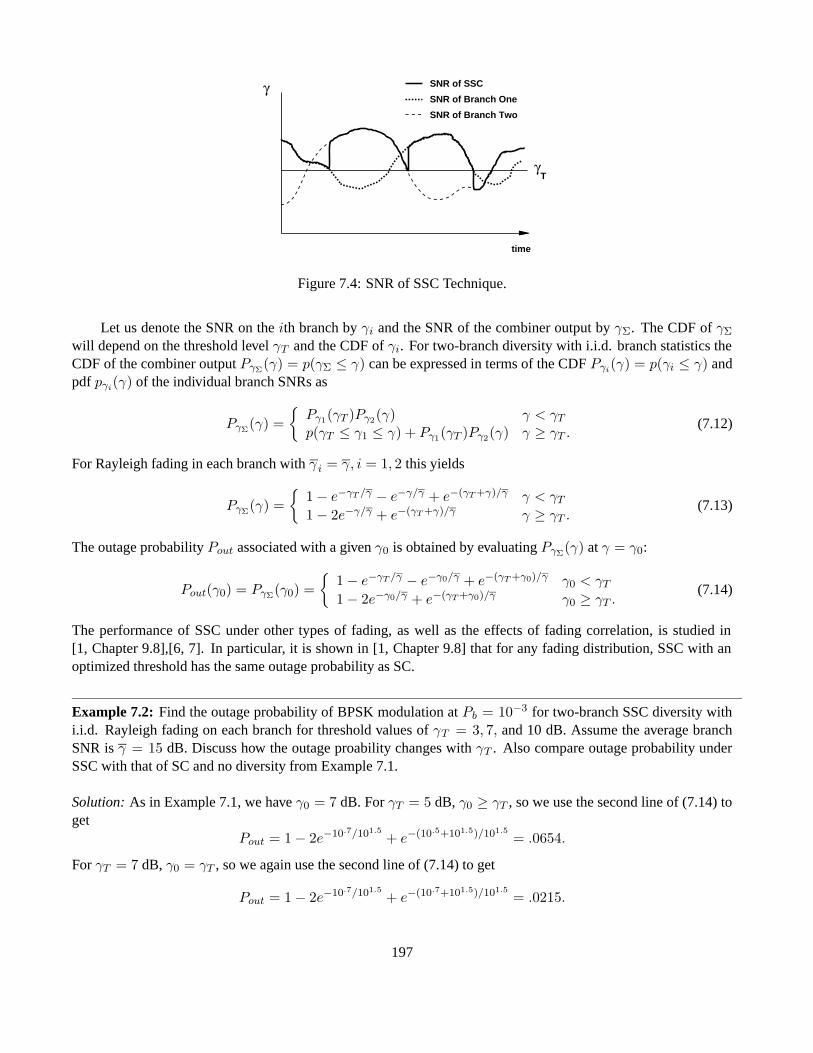
Once a branch is chosen, as long as the SNR on that branch remains above the desired threshold, the combineroutputs that signal. If the SNR on the selected branch falls below the threshold, the combiner switches to anotherbranch. There are several criteria the combiner can use to decide which branch to switch to [5]. The simplestcriterion is to switch randomly to another branch. With only two-branch diversity this is equivalent to switchingto the other branch when the SNR on the active branch falls below γT . This method is called switch and staycombining (SSC). The switching process and SNR associated with SSC is illustrated in Figure 7.4. Since the SSCdoes not select the branch with the highest SNR, its performance is between that of no diversity and ideal SC.

196

time

γ

γT

SNR of Branch Two

SNR of Branch One

SNR of SSC

Figure 7.4: SNR of SSC Technique.

Let us denote the SNR on the ith branch by γi and the SNR of the combiner output by γΣ. The CDF of γΣ

will depend on the threshold level γT and the CDF of γi. For two-branch diversity with i.i.d. branch statistics theCDF of the combiner output PγΣ(γ) = p(γΣ ≤ γ) can be expressed in terms of the CDF Pγi(γ) = p(γi ≤ γ) andpdf pγi(γ) of the individual branch SNRs as

PγΣ(γ) ={

Pγ1(γT )Pγ2(γ) γ < γT

p(γT ≤ γ1 ≤ γ) + Pγ1(γT )Pγ2(γ) γ ≥ γT .(7.12)

For Rayleigh fading in each branch with γ i = γ, i = 1, 2 this yields

PγΣ(γ) ={

1 − e−γT /γ − e−γ/γ + e−(γT +γ)/γ γ < γT

1 − 2e−γ/γ + e−(γT +γ)/γ γ ≥ γT .(7.13)

The outage probability Pout associated with a given γ0 is obtained by evaluating PγΣ(γ) at γ = γ0:

Pout(γ0) = PγΣ(γ0) ={

1 − e−γT /γ − e−γ0/γ + e−(γT +γ0)/γ γ0 < γT

1 − 2e−γ0/γ + e−(γT +γ0)/γ γ0 ≥ γT .(7.14)

The performance of SSC under other types of fading, as well as the effects of fading correlation, is studied in[1, Chapter 9.8],[6, 7]. In particular, it is shown in [1, Chapter 9.8] that for any fading distribution, SSC with anoptimized threshold has the same outage probability as SC.

Example 7.2: Find the outage probability of BPSK modulation at Pb = 10−3 for two-branch SSC diversity withi.i.d. Rayleigh fading on each branch for threshold values of γT = 3, 7, and 10 dB. Assume the average branchSNR is γ = 15 dB. Discuss how the outage proability changes with γT . Also compare outage probability underSSC with that of SC and no diversity from Example 7.1.

Solution: As in Example 7.1, we have γ0 = 7 dB. For γT = 5 dB, γ0 ≥ γT , so we use the second line of (7.14) toget

Pout = 1 − 2e−10.7/101.5+ e−(10.5+101.5)/101.5

= .0654.

For γT = 7 dB, γ0 = γT , so we again use the second line of (7.14) to get

Pout = 1 − 2e−10.7/101.5+ e−(10.7+101.5)/101.5

= .0215.

197

For γT = 10 dB, γ0 < γT , so we use the first line of (7.14) to get

Pout = 1 − e−10/101.5 − e−10.7/101.5+ −e−(10+10.7)/101.5

= .0397.

We see that the outage probability is smaller for γT = 7 dB than for the other two values. At γT = 5 dB thethreshold is too low, so the active branch can be below the target γ0 for a long time before a switch is made, whichcontributes to a large outage probability. At γT = 10 dB the threshold is too high: the active branch will often fallbelow this threshold value, which will cause the combiner to switch to the other antenna even though that otherantenna may have a lower SNR than the active one. This example indicates that the threshold γT that minimizesPout is typically close to the target γ0.

From Example 7.1, SC has Pout = .0215. Thus, γt = 7 dB is the optimal threshold where SSC performs thesame as SC. We also see that performance with an unoptimized threshold can be much worse than SC. However,the performance of SSC under all three thresholds is better than the performance without diversity, derived asPout = .1466 in Example 7.1.

We obtain the pdf of γΣ by differentiating (7.12) relative to γ. Then the average probability of error is obtainedfrom (7.2) with Ps(γ) the probability of symbol error in AWGN and pγΣ(γ) the pdf of the SSC output SNR. Formost fading distributions and coherent modulations, this result cannot be obtained in closed-form and must beevaluated numerically or by approximation. However, for i.i.d. Rayleigh fading we can differentiate (7.13) to get

pγΣ(γ) =

{ (1 − e−γT /γ

)1γ e−γ/γ γ < γT(

2 − e−γT /γ)

1γ e−γ/γ γ ≥ γT .

(7.15)

As with SC, for most fading distributions and coherent modulations, the resulting average probability of erroris not in closed-form and must be evaluated numerically. However, closed-form results do exist for differentialmodulation under i.i.d. Rayleigh fading on each branch. In particular, the average probability of symbol error forDPSK is given by

P b =∫ ∞

0

12e−γpγΣ(γ)dγ =

12(1 + γ)

(1 − e−γT /γ + e−γT e−γT /γ .

)(7.16)

Example 7.3: Find the average probability of error for DPSK modulation under two-branch SSC diversity withi.i.d. Rayleigh fading on each branch for threshold values of γT = 5, 7, and 10 dB. Assume the average branchSNR is γ = 15 dB. Discuss how the average proability of error changes with γT . Also compare average errorprobability under SSC with that of SC and with no diversity.

Solution: Evaluating (7.16) with γ = 15 dB and γT = 3, 7, and 10 dB yields, respectively, P b = .0029, P b =.0023, P b = .0042. As in the previous example, there is an optimal threshold that minimizes average probabilityof error. Setting the threshold too high or too low degrades performance. From (7.11) we have that with SC,P b = .5(1 + 101.5)−1 − .5(2 + 101.5)−1 = 4.56 · 10−4, which is roughly an order of magnitude less than withSSC and an optimized threshold. With no diversity, P b = .5(1 + 101.5)−1 = .0153, which is roughly an order ofmagnitude worse than with two-branch SSC.

198

7.2.4 Maximal Ratio Combining

In SC and SSC, the output of the combiner equals the signal on one of the branches. In maximal ratio combining(MRC) the output is a weighted sum of all branches, so the αis in Figure 7.1 are all nonzero. Since the signals arecophased, αi = aie

−jθi , where θi is the phase of the incoming signal on the ith branch. Thus, the envelope of thecombiner output will be r =

∑Mi=1 airi. Assuming the same noise PSD N0 in each branch yields a total noise PSD

Ntot at the combiner output of Ntot =∑M

i=1 a2i N0. Thus, the output SNR of the combiner is

γΣ =r2

Ntot=

1N0

(∑Mi=1 airi

)2

∑Mi=1 a2

i

. (7.17)

The goal is to chose the αis to maximize γΣ. Intuitively, branches with a high SNR should be weighted morethan branches with a low SNR, so the weights a2

i should be proportional to the branch SNRs r2i /N0. We find the

ais that maximize γΣ by taking partial derivatives of (7.17) or using the Swartz inequality [2]. Solving for theoptimal weights yields a2

i = r2i /N0, and the resulting combiner SNR becomes γΣ =

∑Mi=1 r2

i /N0 =∑M

i=1 γi.Thus, the SNR of the combiner output is the sum of SNRs on each branch. The average combiner SNR increaseslinearly with the number of diversity branches M , in contrast to the diminishing returns associated with the averagecombiner SNR in SC given by (7.10). As with SC, even with Rayleigh fading on all branches, the distribution ofthe combiner output SNR is no longer Rayleigh.

To obtain the distribution of γΣ we take the product of the exponential moment generating or characteristicfunctions. Assuming i.i.d. Rayleigh fading on each branch with equal average branch SNR γ, the distribution ofγΣ is chi-squared with 2M degrees of freedom, expected value γΣ = Mγ, and variance 2Mγ:

pγΣ(γ) =γM−1e−γ/γ

γM (M − 1)!, γ ≥ 0. (7.18)

The corresponding outage probability for a given threshold γ0 is given by

Pout = p(γΣ < γ0) =∫ γ0

0pγΣ(γ)dγ = 1 − e−γ0/γ

M∑k=1

(γ0/γ)k−1

(k − 1)!. (7.19)

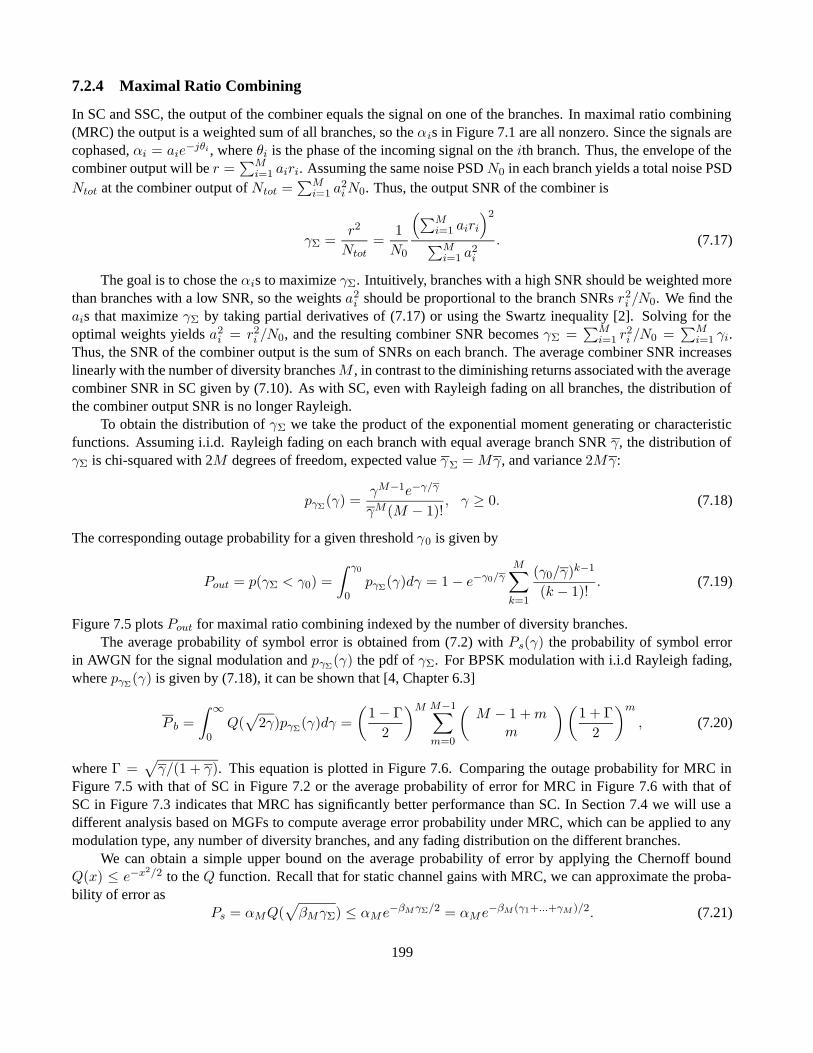
Figure 7.5 plots Pout for maximal ratio combining indexed by the number of diversity branches.The average probability of symbol error is obtained from (7.2) with Ps(γ) the probability of symbol error

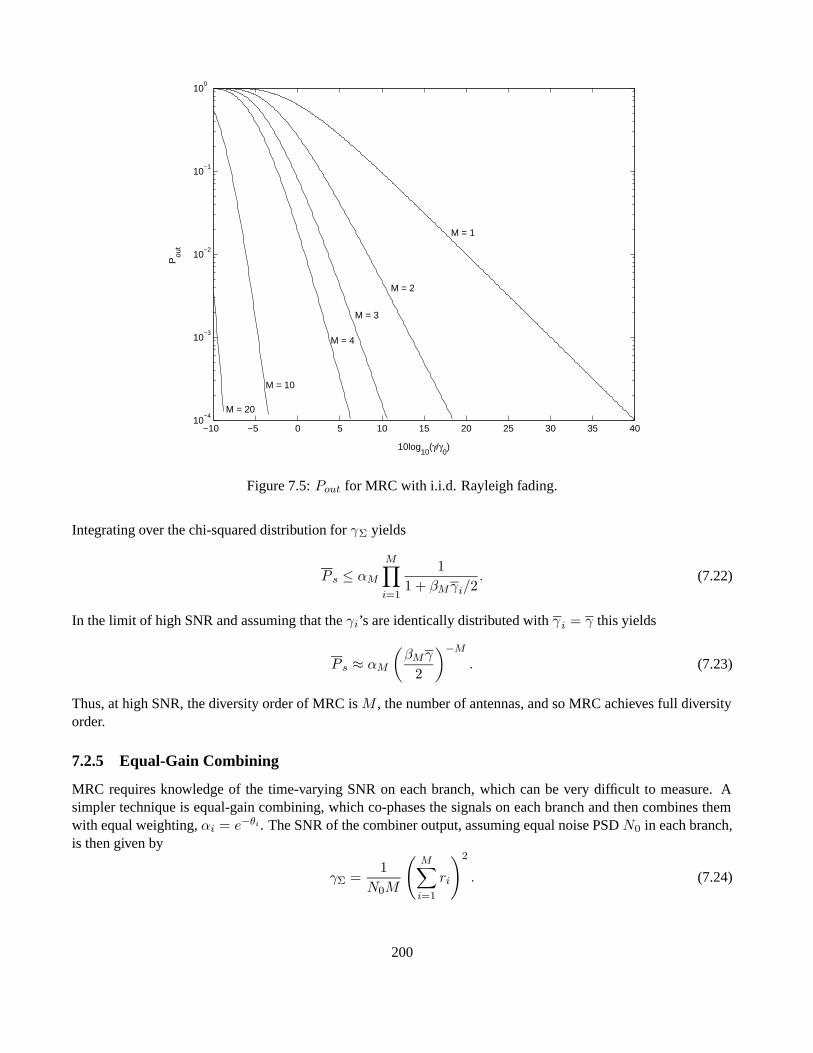
in AWGN for the signal modulation and pγΣ(γ) the pdf of γΣ. For BPSK modulation with i.i.d Rayleigh fading,where pγΣ(γ) is given by (7.18), it can be shown that [4, Chapter 6.3]

P b =∫ ∞

0Q(√

2γ)pγΣ(γ)dγ =(

1 − Γ2

)M M−1∑m=0

(M − 1 + m

m

)(1 + Γ

2

)m

, (7.20)

where Γ =√

γ/(1 + γ). This equation is plotted in Figure 7.6. Comparing the outage probability for MRC inFigure 7.5 with that of SC in Figure 7.2 or the average probability of error for MRC in Figure 7.6 with that ofSC in Figure 7.3 indicates that MRC has significantly better performance than SC. In Section 7.4 we will use adifferent analysis based on MGFs to compute average error probability under MRC, which can be applied to anymodulation type, any number of diversity branches, and any fading distribution on the different branches.

We can obtain a simple upper bound on the average probability of error by applying the Chernoff boundQ(x) ≤ e−x2/2 to the Q function. Recall that for static channel gains with MRC, we can approximate the proba-bility of error as

Ps = αMQ(√

βMγΣ) ≤ αMe−βMγΣ/2 = αMe−βM (γ1+...+γM )/2. (7.21)

199

−10 −5 0 5 10 15 20 25 30 35 4010

−4

10−3

10−2

10−1

100

Pou

t

10log10

(γ/γ0)

M = 1

M = 2

M = 3

M = 4

M = 10

M = 20

Figure 7.5: Pout for MRC with i.i.d. Rayleigh fading.

Integrating over the chi-squared distribution for γΣ yields

P s ≤ αM

M∏i=1

11 + βMγi/2

. (7.22)

In the limit of high SNR and assuming that the γi’s are identically distributed with γ i = γ this yields

P s ≈ αM

(βMγ

2

)−M

. (7.23)

Thus, at high SNR, the diversity order of MRC is M , the number of antennas, and so MRC achieves full diversityorder.

7.2.5 Equal-Gain Combining

MRC requires knowledge of the time-varying SNR on each branch, which can be very difficult to measure. Asimpler technique is equal-gain combining, which co-phases the signals on each branch and then combines themwith equal weighting, αi = e−θi . The SNR of the combiner output, assuming equal noise PSD N0 in each branch,is then given by

γΣ =1

N0M

(M∑i=1

ri

)2

. (7.24)

200

0 5 10 15 20 25 3010

−6

10−5

10−4

10−3

10−2

10−1

100

γb (dB)

Pb

M = 1

M = 2

M = 4

M = 8

M = 10

Figure 7.6: P b for MRC with i.i.d. Rayleigh fading.

The pdf and CDF of γΣ do not exist in closed-form. For i.i.d. Rayleigh fading and two-branch diversity andaverage branch SNR γ, an expression for the CDF in terms of the Q function can be derived as [8, Chapter 5.6][4,Chapter 6.4]

PγΣ(γ) = 1 − e−2γ/γ

√πγ

γe−γ/γ

(1 − 2Q

(√2γ/γ

)). (7.25)

The resulting outage probability is given by

Pout(γ0) = 1 − e−2γR −√πγRe−γR

(1 − 2Q

(√2γR

)), (7.26)

where γR = γ0/γ. Differentiating (7.25) relative to γ yields the pdf

pγΣ(γ) =1γ

e−2γ/γ +√

πe−γ/γ

(1√4γγ

− 1γ

√γ

γ

)(1 − 2Q(

√2γ/γ)

). (7.27)

Substituting this into (7.2) for BPSK yields the average probability of bit error

P b =∫ ∞

0Q(√

2γ)pγΣ(γ)dγ = .5

⎛⎝1 −

√1 −

(1

1 + γ

)2⎞⎠ . (7.28)

It is shown in [8, Chapter 5.7] that performance of EGC is quite close to that of MRC, typically exhibiting less than1 dB of power penalty. This is the price paid for the reduced complexity of using equal gains. A more extensiveperformance comparison between SC, MRC, and EGC can be found in [1, Chapter 9].

201

Example 7.4: Compare the average probability of bit error of BPSK under MRC and EGC two-branch diversitywith i.i.d. Rayleigh fading with average SNR of 10 dB on each branch.

Solution: From (7.20), under MRC we have

P b =

(1 −√

10/112

)2 (2 +

√10/11

)= 1.60 · 10−3.

From (7.28), under EGC we have

P b = .5

⎛⎝1 −

√1 −

(111

)2⎞⎠ = 2.07 · 10−3.

So we see that the performance of MRC and EGC are almost the same.

7.3 Transmitter Diversity

In transmit diversity there are multiple transmit antennas with the transmit power divided among these antennas.Transmit diversity is desirable in systems such as cellular systems where more space, power, and processingcapability is available on the transmit side versus the receive side. Transmit diversity design depends on whether ornot the complex channel gain is known at the transmitter or not. When this gain is known, the system is very similarto receiver diversity. However, without this channel knowledge, transmit diversity gain requires a combination ofspace and time diversity via a novel technique called the Alamouti scheme. We now discuss transmit diversityunder the different assumptions about channel knowledge at the transmitter, assuming the channel gains are knownat the receiver.

7.3.1 Channel Known at Transmitter

Consider a transmit diversity system with M transmit antennas and one receive antenna. We assume the path gainassociated with the ith antenna given by rie

jθi is known at the transmitter. This is refered to as having channel sideinformation (CSI) at the transmitter, or CSIT. Let s(t) denote the transmitted signal with total energy per symbolEs. This signal is multiplied by a complex gain αi = aie

−jθi , 0 ≤ ai ≤ 1 and sent through the ith antenna.This complex multiplication performs both co-phasing and weighting relative to the channel gains. Due to theaverage total energy constraint Es, the weights must satisfy

∑Mi=1 a2

i = 1. The weighted signals transmitted overall antennas are added “in the air”, which leads to a received signal given by

r(t) =M∑i=1

airis(t). (7.29)

Let N0 denote the noise PSD in the receiver.Suppose we wish to set the branch weights to maximize received SNR. Using a similar analysis as in receiver

MRC diversity, we see that the weights ai that achieve the maximum SNR are given by

ai =ri√∑Mi=1 r2

i

, (7.30)

202

and the resulting SNR is

γΣ =Es

N0

M∑i=1

r2i =

M∑i=1

γi, (7.31)

for γi = r2i Es/N0 equal to the branch SNR between the ith transmit antenna and the receive antenna. Thus we

see that transmit diversity when the channel gains are known at the transmitter is very similar to receiver diversitywith MRC: the received SNR is the sum of SNRs on each of the individual branches. In particular, if all antennashave the same gain ri = r, γΣ = Mr2Es/N0, and M -fold increase over just a single antenna transmitting withfull power. Using the Chernoff bound, we see that for static gains

Ps = αMQ(√

βMγΣ) ≤ αMe−βMγΣ/2 = αMe−βM (γ1+...+γM )/2. (7.32)

Integrating over the chi-squared distribution for γΣ yields

P s ≤ αM

M∏i=1

11 + βMγi/2

. (7.33)

In the limit of high SNR and assuming that the γi are identically distributed with γ i = γ this yields

P s ≈ αM

(βMγ

2

)−M

. (7.34)

Thus, at high SNR, the diversity order of transmit diversity with MRC is M , so MRC achieves full diversity order.However, the performance of transmit diversity is worse than receive diversity due to the extra factor of M in thedenominator of (7.34), which results from having to divide the transmit power among all the transmit antennas.Receiver diversity collects energy from all receive antennas, so it does not have this penalty. The analysis for EGCand SC assuming transmitter channel knowledge is the same as under receiver diversity, except that the transmitpower must be divided among all transmit antennas.

The complication of transmit diversity is to obtain the channel phase and, for SC and MRC, the channel gain,at the transmitter. These channel values can be measured at the receiver using a pilot technique and then fed backto the transmitter. Alternatively, in cellular systems with time-division, the base station can measure the channelgain and phase on transmissions from the mobile to the base, and then use these measurements in transmitting backto the mobile, since under time-division the forward and reverse links are reciprocal.

7.3.2 Channel Unknown at Transmitter - The Alamouti Scheme

We now consider the same model as in the previous subsection but assume that the transmitter no longer knowsthe channel gains rie

jθi , so there is no CSIT. In this case it is not obvious how to obtain diversity gain. Consider,for example, a naive strategy whereby for a two-antenna system we divide the transmit energy equally betweenthe two antennas. Thus, the transmit signal on antenna i will be si(t) =

√.5s(t) for s(t) the transmit signal with

energy per symbol Es. Assume each antenna has a complex Gaussian channel gain hi = riejθi , i = 1, 2 with mean

zero and variance one. The received signal is then

r(t) =√

.5(h1 + h2)s(t). (7.35)

Note that h1 + h2 is the sum of two complex Gaussian random variables, and is thus a complex Gaussian as wellwith mean equal to the sum of means (zero) and variance equal to the sum of variances (2). Thus

√.5(h1 + h2)

is a complex Gaussian random variable with mean zero and variance one, so the received signal has the same

203

distribution as if we had just used one antenna with the full energy per symbol. In other words, we have obtainedno performance advantage from the two antennas, since we could not divide our energy intelligently between themor obtain coherent combining through co-phasing.

Transmit diversity gain can be obtained even in the absence of channel information with an appropriate schemeto exploit the antennas. A particularly simple and prevalent scheme for this diversity that combines both space andtime diversity was developed by Alamouti in [9]. Alamouti’s scheme is designed for a digital communicationsystem with two-antenna transmit diversity. The scheme works over two symbol periods where it is assumed thatthe channel gain is constant over this time. Over the first symbol period two different symbols s1 and s2 each withenergy Es/2 are transmitted simultaneously from antennas 1 and 2, respectively. Over the next symbol periodsymbol −s∗2 is transmitted from antenna 1 and symbol s∗1 is transmitted from antenna 2, each with symbol energyEs/2.

Assume complex channel gains hi = riejθi , i = 1, 2 between the ith transmit antenna and the receive antenna.

The received symbol over the first symbol period is y1 = h1s1+h2s2+n1 and the received symbol over the secondsymbol period is y2 = −h1s

∗2 +h2s

∗1 +n2, where ni, i = 1, 2 is the AWGN noise sample at the receiver associated

with the ith symbol transmission. We assume the noise sample has mean zero and power N .The receiver uses these sequentially received symbols to form the vector y = [y1y

∗2]

T given by

y =[

h1 h2

h∗2 −h∗

1

] [s1

s2

]+[

n1

n∗2

]= HAs + n,

where s = [s1s2]T , n = [n1n2]T , and

HA =[

h1 h2

h∗2 −h∗

1

].

Let us define the new vector z = HHAy. The structure of HA implies that

HHA HA = (|h2

1| + |h22|)I2, (7.36)

is diagonal, and thusz = [z1 z2]T = (|h2

1| + |h22|)I2s + n, (7.37)

where n = HHAn is a complex Gaussian noise vector with mean zero and covariance matrix E[nn∗] = (|h2

1| +|h2

2|)NI2 The diagonal nature of z effectively decouples the two symbol transmissions, so that each component ofz corresponds to one of the transmitted symbols:

zi = (|h21| + |h2

2|)si + ni, i = 1, 2. (7.38)

The received SNR thus corresponds to the SNR for zi given by

γi =(|h2

1| + |h22|)Es

2N0, (7.39)

where the factor of 2 comes from the fact that si is transmitted using half the total symbol energy Es. The receivedSNR is thus equal to the sum of SNRs on each branch, identical to the case of transmit diversity with MRCassuming that the channel gains are known at the transmitter. Thus, the Alamouti scheme achieves a diversityorder of 2, the maximum possible for a two-antenna transmit system, despite the fact that channel knowledge isnot available at the transmitter. However, it only achieves an array gain of 1, whereas MRC can achieve an arraygain and a diversity gain of 2. The Alamouti scheme can be generalized for M > 2 when the constellations arereal, but if the contellations are complex the generalization is only possible with a reduction in code rates [10].

204

7.4 Moment Generating Functions in Diversity Analysis

In this section we use the MGFs introduced in Section 6.3.3 to greatly simplify the analysis of average error proba-bility under diversity. The use of MGFs in diversity analysis arises from the difficulty in computing the pdf pγΣ(γ)of the combiner SNR γΣ. Specifically, although the average probability of error and outage probability associatedwith diversity combining are given by the simple formulas (7.2) and (7.3), these formulas require integration overthe distribution pγΣ(γ). This distribution is often not in closed-form for an arbitrary number of diversity brancheswith different fading distributions on each branch, regardless of the combining technique that is used. The pdf forpγΣ(γ) is often in the form of an infinite-range integral, in which case the expressions for (7.2) and (7.3) becomedouble integrals that can be difficult to evaluate numerically. Even when pγΣ(γ) is in closed form, the correspond-ing integrals (7.2) and (7.3) may not lead to closed-form solutions and may be difficult to evaluate numerically.A large body of work over many decades has addressed approximations and numerical techniques to compute theintegrals associated with average probability of symbol error for different modulations, fading distributions, andcombining techniques (see [11] and the references therein). Expressing the average error probability in terms ofthe MGF for γΣ instead of its pdf often eliminates these integration difficulties. Specifically, when the diversityfading paths that are independent but not necessarily identically distributed, the average error probability based onthe MGF of γΣ is typically in closed-form or consists of a single finite-range integral that can be easily computednumerically.

The simplest application of MGFs in diversity analysis is for coherent modulation with MRC, so this is treatedfirst. We then discuss the use of MGFs in the analysis of average error probability under EGC and SC.

7.4.1 Diversity Analysis for MRC

The simplicity of using MGFs in the analysis of MRC stems from the fact that, as derived in Section 7.2.4, thecombiner SNR γΣ is the sum of theγi’s, the branch SNRS:

γΣ =M∑i=1

γi. (7.40)

As in the analysis of average error probability without diversity (Section 6.3.3), let us again assume that theprobability of error in AWGN for the modulation of interest can be expressed either as an exponential function ofγs, as in (6.67), or as a finite range integral of such a function, as in (6.68).

We first consider the case where Ps is in the form of (6.67). Then the average probability of symbol errorunder MRC is

P s =∫ ∞

0c1 exp[−c2γ]pγΣ(γ)dγ. (7.41)

We assume that the branch SNRs are independent, so that their joint pdf becomes a product of the individual pdfs:pγ1,...,γM (γ1, . . . , γM ) = pγ1(γ1) . . . pγM (γM ). Using this factorization and substituting γ = γ1 + . . . + γM in(7.41) yields

P s = c1

∫ ∞

0

∫ ∞

0· · ·

∫ ∞

0︸ ︷︷ ︸M−fold

exp[−c2(γ1 + . . . + γM )]pγ1(γ1) . . . pγM (γM )dγ1 . . . dγM . (7.42)

Now using the product forms exp[−β(γ1+. . .+γM )] =∏M

i=1 exp[−βγi] and pγ1(γ1) . . . pγM (γM ) =∏M

i=1 pγi(γi)in (7.42) yields

P s = c1

∫ ∞

0

∫ ∞

0· · ·∫ ∞

0︸ ︷︷ ︸M−fold

M∏i=1

exp[−c2γi]pγi(γi)dγi. (7.43)

205

Finally, switching the order of integration and multiplication in (7.43) yields our desired final form

P s = c1

M∏i=1

∫ ∞

0exp[−c2γi]pγi(γi)dγi = c1

M∏i=1

Mγi(−c2). (7.44)

Thus, the average probability of symbol error is just the product of MGFs associated with the SNR on each branch.Similary, when Ps is in the form of (6.68), we get

P s =∫ ∞

0

∫ B

Ac1 exp[−c2(x)γ]dxpγΣ(γ)dγ =

∫ ∞

0

∫ ∞

0· · ·

∫ ∞

0︸ ︷︷ ︸M−fold

∫ B

Ac1

M∏i=1

exp[−c2(x)γi]pγi(γi)dγi. (7.45)

Again switching the order of integration and multiplication yields our desired final form

P s = c1

∫ B

A

M∏i=1

∫ ∞

0exp[−c2(x)γi]pγi(γi)dγi = c1

∫ B

A

M∏i=1

Mγi(−c2(x))dx. (7.46)

Thus, the average probability of symbol error is just a single finite-range integral of the product of MGFs associatedwith the SNR on each branch. The simplicity of (7.44) and (7.46) are quite remarkable, given that these expressionsapply for any number of diversity branches and any type of fading distribution on each branch, as long as the branchSNRs are independent.

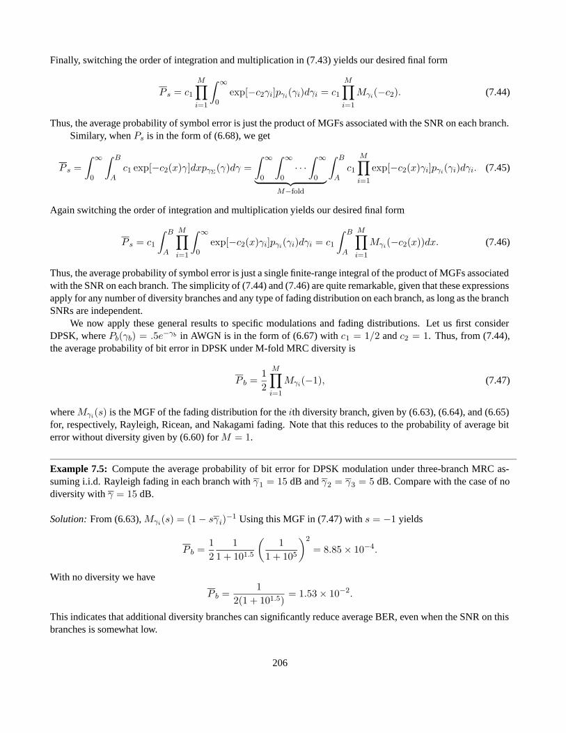
We now apply these general results to specific modulations and fading distributions. Let us first considerDPSK, where Pb(γb) = .5e−γb in AWGN is in the form of (6.67) with c1 = 1/2 and c2 = 1. Thus, from (7.44),the average probability of bit error in DPSK under M-fold MRC diversity is

P b =12

M∏i=1

Mγi(−1), (7.47)

where Mγi(s) is the MGF of the fading distribution for the ith diversity branch, given by (6.63), (6.64), and (6.65)for, respectively, Rayleigh, Ricean, and Nakagami fading. Note that this reduces to the probability of average biterror without diversity given by (6.60) for M = 1.

Example 7.5: Compute the average probability of bit error for DPSK modulation under three-branch MRC as-suming i.i.d. Rayleigh fading in each branch with γ1 = 15 dB and γ2 = γ3 = 5 dB. Compare with the case of nodiversity with γ = 15 dB.

Solution: From (6.63), Mγi(s) = (1 − sγi)−1 Using this MGF in (7.47) with s = −1 yields

P b =12

11 + 101.5

(1

1 + 105

)2

= 8.85 × 10−4.

With no diversity we have

P b =1

2(1 + 101.5)= 1.53 × 10−2.

This indicates that additional diversity branches can significantly reduce average BER, even when the SNR on thisbranches is somewhat low.

206

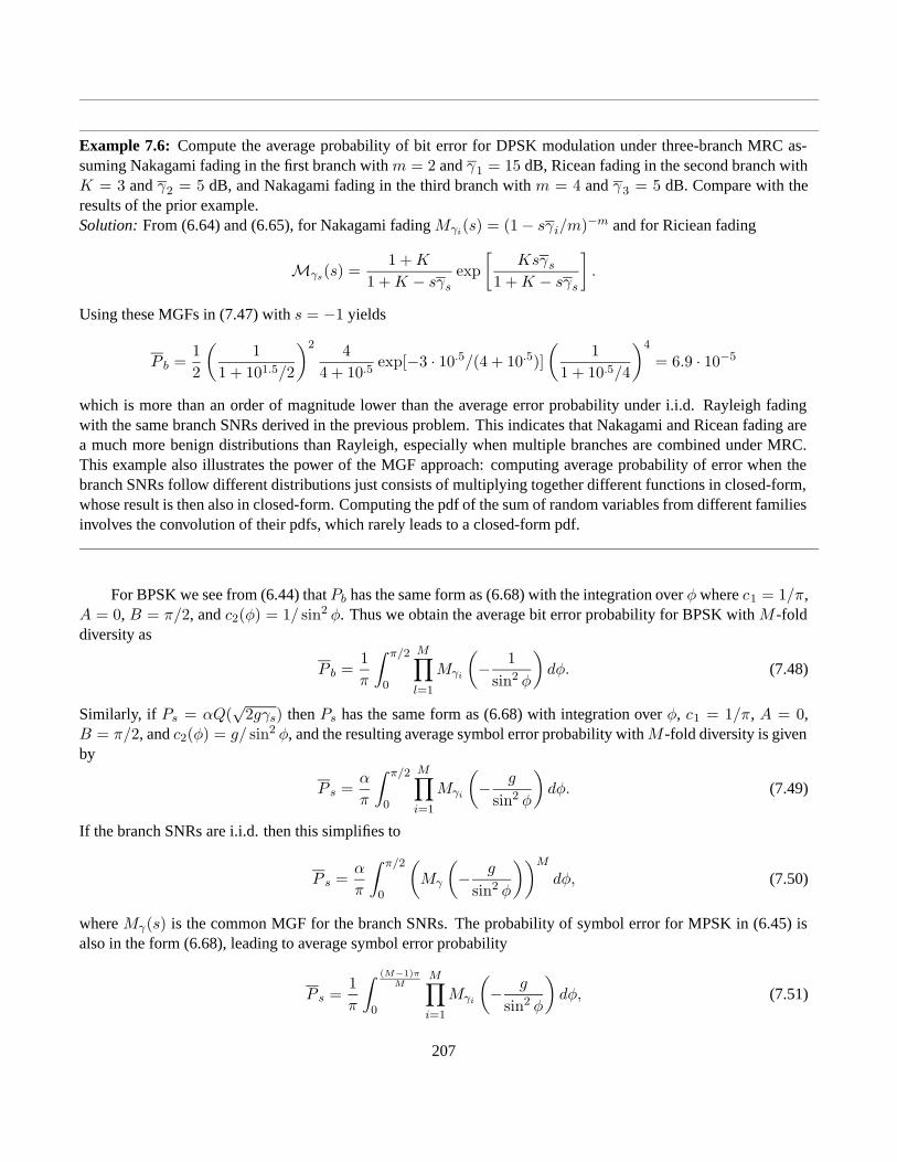
Example 7.6: Compute the average probability of bit error for DPSK modulation under three-branch MRC as-suming Nakagami fading in the first branch with m = 2 and γ1 = 15 dB, Ricean fading in the second branch withK = 3 and γ2 = 5 dB, and Nakagami fading in the third branch with m = 4 and γ3 = 5 dB. Compare with theresults of the prior example.Solution: From (6.64) and (6.65), for Nakagami fading Mγi(s) = (1 − sγi/m)−m and for Riciean fading

Mγs(s) =1 + K

1 + K − sγs

exp[

Ksγs

1 + K − sγs

].

Using these MGFs in (7.47) with s = −1 yields

P b =12

(1

1 + 101.5/2

)2 44 + 10.5

exp[−3 · 10.5/(4 + 10.5)](

11 + 10.5/4

)4

= 6.9 · 10−5

which is more than an order of magnitude lower than the average error probability under i.i.d. Rayleigh fadingwith the same branch SNRs derived in the previous problem. This indicates that Nakagami and Ricean fading area much more benign distributions than Rayleigh, especially when multiple branches are combined under MRC.This example also illustrates the power of the MGF approach: computing average probability of error when thebranch SNRs follow different distributions just consists of multiplying together different functions in closed-form,whose result is then also in closed-form. Computing the pdf of the sum of random variables from different familiesinvolves the convolution of their pdfs, which rarely leads to a closed-form pdf.

For BPSK we see from (6.44) that Pb has the same form as (6.68) with the integration over φ where c1 = 1/π,A = 0, B = π/2, and c2(φ) = 1/ sin2 φ. Thus we obtain the average bit error probability for BPSK with M -folddiversity as

P b =1π

∫ π/2

0

M∏l=1

Mγi

(− 1

sin2 φ

)dφ. (7.48)

Similarly, if Ps = αQ(√

2gγs) then Ps has the same form as (6.68) with integration over φ, c1 = 1/π, A = 0,B = π/2, and c2(φ) = g/ sin2 φ, and the resulting average symbol error probability with M -fold diversity is givenby

P s =α

π

∫ π/2

0

M∏i=1

Mγi

(− g

sin2 φ

)dφ. (7.49)

If the branch SNRs are i.i.d. then this simplifies to

P s =α

π

∫ π/2

0

(Mγ

(− g

sin2 φ

))M

dφ, (7.50)

where Mγ(s) is the common MGF for the branch SNRs. The probability of symbol error for MPSK in (6.45) isalso in the form (6.68), leading to average symbol error probability

P s =1π

∫ (M−1)πM

0

M∏i=1

Mγi

(− g

sin2 φ

)dφ, (7.51)

207

where g = sin2(

πM

). For i.i.d. fading this simplifies to

P s =1π

∫ (M−1)πM

0

(Mγ

(− g

sin2 φ

))M

dφ. (7.52)

Example 7.7: Find an expression for the average symbol error probability for 8PSK modulation for two-branchMRC combining, where each branch is Rayleigh fading with average SNR of 20 dB.

Solution: The MGF for Rayleigh is Mγi(s) = (1− sγi)−1. Using this MGF in (7.52) with s = − sin2 π/8/ sin2 φand γ = 100 yields

P s =1π

∫ 7π/8

0

⎛⎝ 1

1 + 100 sin2 π/8

sin2 φ

⎞⎠2

dφ.

This expression does not lead to a closed-form solution and so must be evaluated numerically, which results inP s = 1.56 · 10−3.

We can use similar techniques to extend the derivation of the exact error probability for MQAM in fading,given by (7.53), to include MRC diversity. Specifically, we first integrate the expression for Ps in AWGN, ex-pressed in (6.80) using the alternate representation of Q and Q2, over the distribution of γΣ. Since γΣ =

∑i γi

and the SNRs are independent, the exponential function and distribution in the resulting expression can be writtenin product form. Then we use the same reordering of integration and multiplication used above in the MPSKderivation. The resulting average probability of symbol error for MQAM modulation with MRC combining isgiven by

P s =4π

(1 − 1√

M

) ∫ π/2

0

M∏i=1

Mγi

(− g

sin2 φ

)dφ− 4

π

(1 − 1√

M

)2 ∫ π/4

0

M∏i=1

Mγi

(− g

sin2 φ

)dφ. (7.53)

More details on the use of MGFs to obtain average probability of error under M -fold MRC diversity for a broadclass of modulations can be found in [10, Chapter 9.2].

7.4.2 Diversity Analysis for EGC and SC

MGFs are less useful in the analysis of EGC and SC than in MRC. The reason is that with MRC, γΣ =∑

i γi,so exp[−c2γΣ] =

∏i exp[−c2γi] This factorization leads directly to the simple formulas whereby probability of

symbol error is based on a product of MGFs associated with each of the branch SNRs. Unfortunately, neither EGCnor SC leads to this type of factorization. However, working with the MGF of γΣ can sometimes lead to simplerresults than working directly with its pdf. This is illustrated in [1, Chapter 9.3.3], where the exact probability ofsymbol error for MPSK is obtained based on the characteristic function associated with each branch SNR, wherethe characteristic function is just the MGF evaluated at s = j2πf , i.e. it is the Fourier transform of the pdf. Theresulting average error probability, given by [10, Equation 9.78], is a finite-range integral over a sum of closed-formexpressions, and is thus easily evaluated numerically.

208

7.4.3 Diversity Analysis for Noncoherent and Differentially Coherent Modulation

A similar approach to determining the average symbol error probability of noncoherent and differentially coherentmodulations with diversity combining is presented in [12, 10]. This approach differs from that of the coherentmodulation case in that it relies on an alternate form of the Marcum Q-function instead of the Gaussian Q-function,since the BER of noncoherent and differentially coherent modulations in AWGN are given in terms of the MarcumQ-function. Otherwise the approach is essentially the same as in the coherent case, and leads to BER expressionsinvolving a single finite-range integral that can be readily evaluated numerically. More details on this approach canbe found in [12] and [10].

209

Bibliography

[1] M. Simon and M.-S. Alouini, Digital Communication over Fading Channels A Unified Approach to Perfor-mance Analysis. Wiley, 2000.

[2] W. Lee, Mobile Communications Engineering. New York: McGraw-Hill, 1982.

[3] J. Winters, “Signal acquisition and tracking with adaptive arrays in the digital mobile radio system is-54 withflat fading,” IEEE Trans. Vehic. Technol., vol. 43, pp. 1740–1751, Nov. 1993.

[4] G. L. Stuber, Principles of Mobile Communications, 2nd Ed. Kluwer Academic Publishers, 2001.

[5] M. Blanco and K. Zdunek, “Performance and optimization of switched diversity systems for the detection ofsignals with rayleigh fading,” IEEE Trans. Commun., pp. 1887–1895, Dec. 1979.

[6] A. Abu-Dayya and N. Beaulieu, “Switched diversity on microcellular ricean channels,” IEEE Trans. Vehic.Technol., pp. 970–976, Nov. 1994.

[7] A. Abu-Dayya and N. Beaulieu, “Analysis of switched diversity systems on generalized-fading channels,”IEEE Trans. Commun., pp. 2959–2966, Nov. 1994.

[8] M. Yacoub, Principles of Mobile Radio Engineering. CRC Press, 1993.

[9] S. Alamouti, “A simple transmit diversity technique for wireless communications,” IEEE J. Select. AreasCommun., pp. 1451–1458, Oct. 1998.

[10] A. Paulraj, R. Nabar, and D. Gore, Introduction to Space-Time Wireless Communications. Cambridge, Eng-land: Cambridge University Press, 2003.

[11] M. K. Simon and M. -S. Alouini, “A unified approach to the performance analysis of digital communicationsover generalized fading channels,” Proc. IEEE, vol. 86, pp. 1860–1877, September 1998.

[12] M. K. Simon and M. -S. Alouini, “A unified approach for the probability of error for noncoherent and dif-ferentially coherent modulations over generalized fading channels,” IEEE Trans. Commun., vol. COM-46,pp. 1625–1638, December 1998.

210

Chapter 7 Problems

1. Find the outage probability of QPSK modulation at Ps = 10−3 for a Rayleigh fading channel with SCdiversity for M = 1 (no diversity), M = 2, and M = 3. Assume branch SNRs γ1 = 10 dB, γ2 = 15 dB,and γ3 = 20 dB.

2. Plot the pdf pγΣ(γ) given by (7.9) for the selection-combiner SNR in Rayleigh fading with M branch di-versity assuming M = 1, 2, 4, 8, and 10. Assume each branch has average SNR of 10 dB. Your plot shouldbe linear on both axes and should focus on the range of linear γ values 0 ≤ γ ≤ 60. Discuss how the pdfchanges with increasing M and why that leads to lower probability of error.

3. Derive the average probability of bit error for DPSK under SC with i.i.d. Rayleigh fading on each branch asgiven by (7.11).

4. Derive a general expression for the CDF of the SSC output SNR for branch statistics that are not i.i.d. andshow that it reduces to (7.12) for i.i.d. branch statistics. Evaluate your expression assuming Rayleigh fadingin each branch with different average SNRs γ1 and γ2.

5. Derive the average probability of bit error for DPSK under SSC with i.i.d. Rayleigh fading on each branchas given by (7.16).

6. Compare the average probability of bit error for DPSK under no diversity, SC, and SSC, assuming i.i.d.Rayleigh fading on each branch and an average branch SNR of 10 dB and of 20 dB. How does the relativeperformance change as the branch SNR increases.

7. Plot the average probability of bit error for DPSK under SSC with M = 2, 3, and 4, assuming i.i.d. Rayleighfading on each branch and an average branch SNR ranging from 0 to 20 dB.

8. Show that the weights αi that maximize γΣ under MRC are α2i = r2

i /N for N the common noise power oneach branch. Also show that with these weights, γΣ =

∑i γi.

9. This problem illustrates that you can get performance gains from diversity combining even without fading,due to noise averaging. Consider an AWGN channel with N branch diversity combining and γi = 10 dBper branch. Assume MQAM modulation with M = 4 and use the approximation Pb = .2e−1.5γ/(M−1) forbit error probability, where γ is the received SNR.

(a) Find Pb for N = 1.

(b) Find N so that under MRC, Pb < 10−6.

10. Derive the average probability of bit error for BPSK under MRC with i.i.d. Rayleigh fading on each branchas given by (7.20).

11. Derive the average probability of bit error for BPSK under EGC with i.i.d. Rayleigh fading on each branchas given by (7.28).

12. Compare the average probability of bit error for BPSK modulation under no diversity, two-branch SC, two-branch SSC, two-branch EGC, and two-branch MRC. Assume i.i.d. Rayleigh fading on each branch withequal branch SNR of 10 dB and of 20 dB. How does the relative performance change as the branch SNRincreases.

211

13. Plot the average probability of bit error for BPSK under both MRC and EGC assuming two-branch diversitywith i.i.d. Rayleigh fading on each branch and average branch SNR ranging from 0 to 20 dB. What is themaximum dB penalty of EGC as compared to MRC?

14. Compare the outage probability of BPSK modulation at Pb = 10−3 under MRC and under EGC assumingtwo-branch diversity with i.i.d. Rayleigh fading on each branch and average branch SNR γ=10 dB.

15. Compare the average probability of bit error for BPSK under MRC and under EGC assuming two-branchdiversity with i.i.d. Rayleigh fading on each branch and average branch SNR γ=10 dB.

16. Compute the average BER of a channel with two-branch transmit diversity under the Alamouti scheme,assuming the branch SNR is 10 dB.

17. Consider a fading distribution p(γ) where∫∞0 p(γ)e−xγdγ = .01γ/

√x. Find the average Pb for a BPSK

modulated signal where the receiver has 2-branch diversity with MRC combining, and each branch has anaverage SNR of 10 dB and experiences independent fading with distribution p(γ).

18. Consider a fading channel with BPSK modulation, 3 branch diversity with MRC, where each branch experi-ences independent fading with an average received SNR of 15 dB. Compute the average BER of this channelfor Rayleigh fading and for Nakagami fading with m = 2 (Using the alternate Q function representationgreatly simplifies this computation, at least for Nakagami fading).

19. Plot the average probability of error as a function of branch SNR for a two branch MRC system with BPSKmodulation, where the first branch has Rayleigh fading and the second branch has Nakagami-m fading withm=2. Assume the two branches have the same average SNR, and your plots should have that average branchSNR ranging from 5 to 20 dB.

20. Plot the average probability of error as a function of branch SNR for an M -branch MRC system with 8PSKmodulation for M = 1, 2, 4, 8. Assume each branch has Rayleigh fading with the same average SNR. Yourplots should have an SNR that ranges from 5 to 20 dB.

21. Derive the average probability of symbol error for MQAM modulation under MRC diversity given by (7.53)from the probability of error in AWGN (6.80) by utilizing the alternate representation of Q and Q2,

22. Compare the average probability of symbol error for 16PSK and 16QAM modulation, assuming three-branchMRC diversity with Rayleigh fading on the first branch and Ricean fading on the second and third brancheswith K = 2. Assume equal average branch SNRs of 10 dB.

23. Plot the average probability of error as a function of branch SNR for an M -branch MRC system with 16QAMmodulation for M = 1, 2, 4, 8. Assume each branch has Rayleigh fading with the same average SNR. Yourplots should have an SNR that ranges from 5 to 20 dB.

212