Want high rates, high spectral efficiency, high power efficiency, robust to channel, cheap.
Amplitude/Phase Modulation (MPSK,MQAM)Information encoded in amplitude/phase More spectrally efficient than frequency modulationIssues: differential encoding, pulse shaping, bit mapping.
Frequency Modulation (FSK)Information encoded in frequencyContinuous phase (CPFSK) special case of FMBandwidth determined by Carson’s rule (pulse shaping)More robust to channel and amplifier nonlinearities
٢
Slide 3Wireless Communications
Amplitude/Phase Modulation
Signal over ith symbol period:
Pulse shape g(t) typically NyquistSignal constellation defined by (si1,si2) pairsCan be differentially encodedM values for (si1,si2)log2 M bits per symbol
Ps depends onMinimum distance dmin (depends on s)# of nearest neighbors MApproximate expression:
)2sin()()2cos()()( 0201 tftgstftgsts cici
sMMs QP
Slide 4Wireless Communications
The received SNR is given by
In system with interference, we use signal to interference plus noise power ratio (SINR)- (PI power of interference)
SNR is often expressed in term of Es or Eb
Signal to noise ratio
BNPSNR r 0/
I
r
PBNPSNR
0
b
b
s
s
I
r
BTNE
BTNE
BNPSNR
000
٣
Slide 5Wireless Communications
with
For raised cosine (=1), Ts = 1/B then SNR = ES /N0
In general Ts = k/B or k.SNR = ES /N0
For M-array signaling:
and
Signal to noise ratio
0NEb
b 0NEs
s
Ms
b2log
MPP s
b2log
Slide 6Wireless Communications
For BPSK
For QPSK
or
For MPSK
Error Probability for PSK
bb QP 2
2/2 ss QP
MQP ss /sin22
211 ss QP
٤
Slide 7Wireless Communications
For MPAM
For MQAM
And using the nearest neabour approximation
Error Probability
1
6122M
QMMP s
s
1
312M
QMMP s
s
2
131211
M
QMMP s
s
Slide 8Wireless Communications
Example 1: Find the bit error probability Pb and symbol error probability Ps of QPSK assuming γb = 7dB. Compare the exact Pbwith the approximation Pb = Ps/2 based on the assumption of Gray coding. Finally, compute Ps based on the nearest-neighbor bound using γs = 2γb, and compare with the exact Ps.
Solution: We have γb = 107/10 = 5.012,
The exact symbol error rate
The approximate symbol error rate
410*726.7024.102 QQP bb
32210*55.102.101111 QQP ss
310*545.12 bs PP
٥
Slide 9Wireless Communications
Example 2: Compare the probability of bit error for 8PSK and 16PSK assuming γb = 15 dB and using the Ps approximation
For 8-PSK, γs = (log2 8) · 1015/10 = 94.87
Pb = Ps /3 = 4.52 · 10−8.
For 16-PSK we have γs = (log2 16) · 1015/10 = 126.49
Pb = Ps /4 = 4.79 · 10−4.
The error in 16-PSK is much larger (WHY?)
710.355.18/sin74.1892 QPs
310.916.116/sin98.2522 QPs
Slide 10Wireless Communications
Example 3: For 16QAM with γb = 15 dB , compare the exact probability of symbol error with the nearest neighbor approximation , and with the symbol error probability for 16PSK with the same γb that was obtained in the previous example
The exact symbol error rate is
And the approximate
7
2
10*37.715
49.126*3414211
QPs
710*68.315
49.126*34142
QPs
٦
Slide 11Wireless Communications
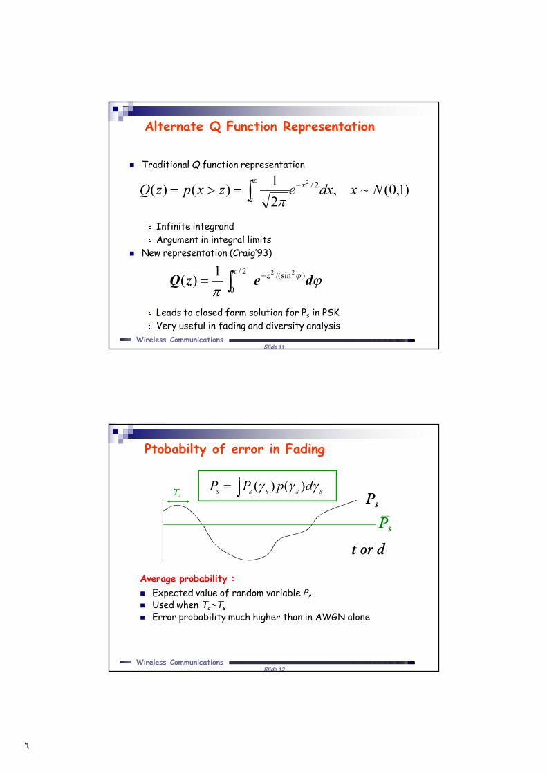
Alternate Q Function Representation
Traditional Q function representation
Infinite integrandArgument in integral limits
New representation (Craig’93)
Leads to closed form solution for Ps in PSKVery useful in fading and diversity analysis
)1,0(~,21)()( 2/2 NxdxezxpzQ x
z
dezQ z )/(sin2/
0
221)(
Slide 12Wireless Communications
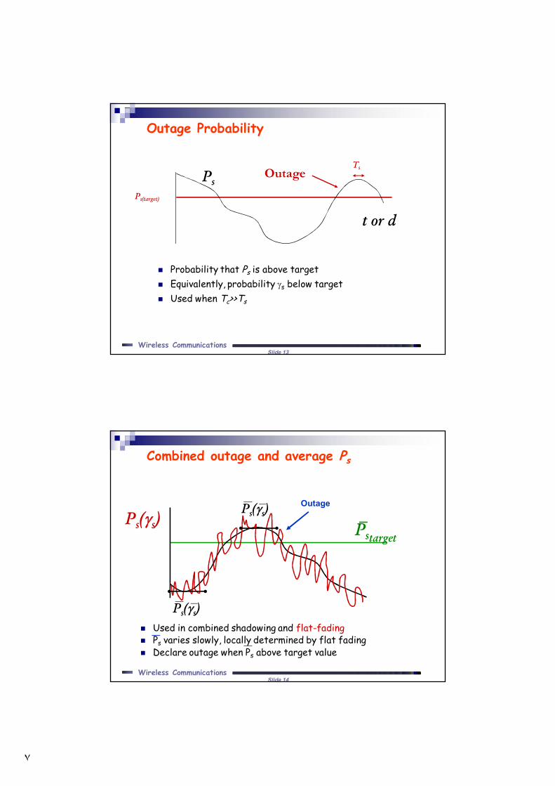
Ptobabilty of error in Fading
Average probability : Expected value of random variable Ps Used when Tc~Ts Error probability much higher than in AWGN alone
sssss dpPP )()( Ps
Ps
Ts
t or d
٧
Slide 13Wireless Communications
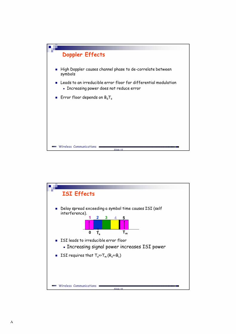
Outage Probability
Probability that Ps is above target Equivalently, probability s below target Used when Tc>>Ts
PsPs(target)
OutageTs
t or d
Slide 14Wireless Communications
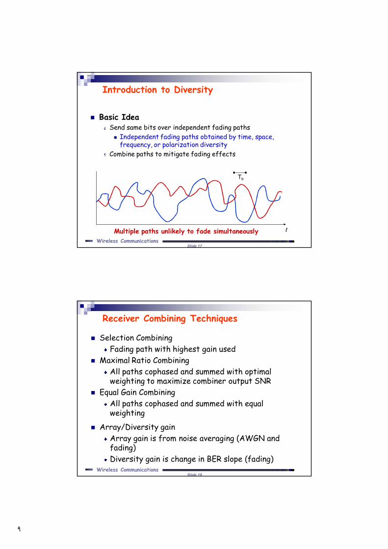
Combined outage and average Ps
Used in combined shadowing and flat-fading Ps varies slowly, locally determined by flat fading Declare outage when Ps above target value
Ps(s) Pstarget
Ps(s)
Ps(s)
Outage
٨
Slide 15Wireless Communications
Doppler Effects
High Doppler causes channel phase to de-correlate between symbols
Leads to an irreducible error floor for differential modulationIncreasing power does not reduce error
Error floor depends on BdTs
Slide 16Wireless Communications
Delay spread exceeding a symbol time causes ISI (self interference).
ISI leads to irreducible error floorIncreasing signal power increases ISI power
ISI requires that Ts>>Tm (Rs<<Bc)
ISI Effects
0 Tm
1 2 3 4 5
Ts
٩
Slide 17Wireless Communications
Introduction to Diversity
Basic IdeaSend same bits over independent fading paths Independent fading paths obtained by time, space,
frequency, or polarization diversityCombine paths to mitigate fading effects
Tb
tMultiple paths unlikely to fade simultaneously
Slide 18Wireless Communications
Selection CombiningFading path with highest gain used
Maximal Ratio CombiningAll paths cophased and summed with optimal weighting to maximize combiner output SNR
Equal Gain CombiningAll paths cophased and summed with equal weighting
Array/Diversity gainArray gain is from noise averaging (AWGN and fading)Diversity gain is change in BER slope (fading)
Receiver Combining Techniques
١٠
Slide 19Wireless Communications
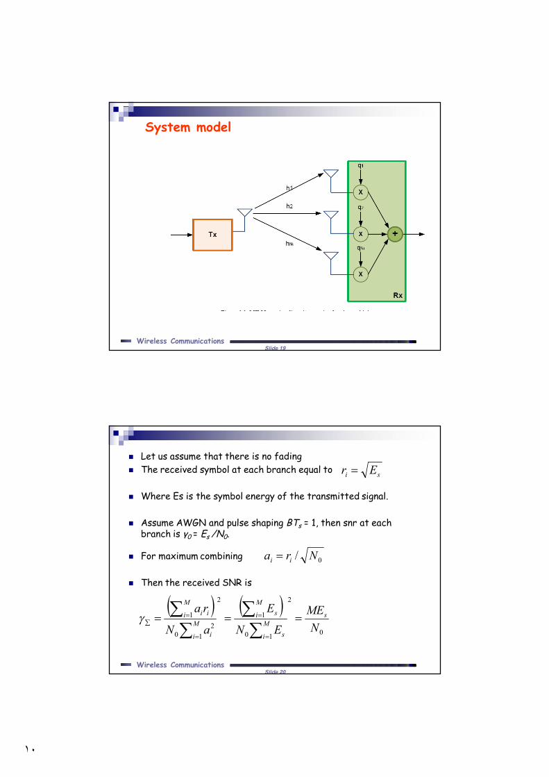
System model
Slide 20Wireless Communications
Let us assume that there is no fading The received symbol at each branch equal to
Where Es is the symbol energy of the transmitted signal.
Assume AWGN and pulse shaping BTs = 1, then snr at each branch is γ0 = Es /N0.
For maximum combining
Then the received SNR is
si Er
0/ Nra ii
0
2
10
1
2
12
0
1
NME
EN
E
aN
ras
M
i s
M
i sM
i i
M
i ii
١١
Slide 21Wireless Communications
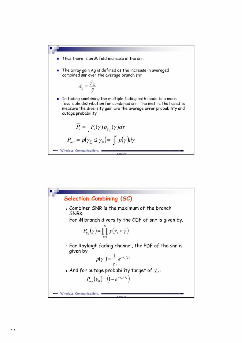
Thus there is an M fold increase in the snr.
The array gain Ag is defined as the increase in averaged combined snr over the average branch snr
In fading combining the multiple fading path leads to a more favorable distribution for combined snr. The metric that used to measure the diversity gain are the average error probability and outage probability
gA
dpPP ss )()(
00 dppPout
Slide 22Wireless Communications
Combiner SNR is the maximum of the branch SNRs.For M branch diversity the CDF of snr is given by.
For Rayleigh fading channel, the PDF of the snr is given by
And for outage probability target of γ0 .
Selection Combining (SC)
M
iipP
1
iiepi
i
/1
iePout /
001
١٢
Slide 23Wireless Communications
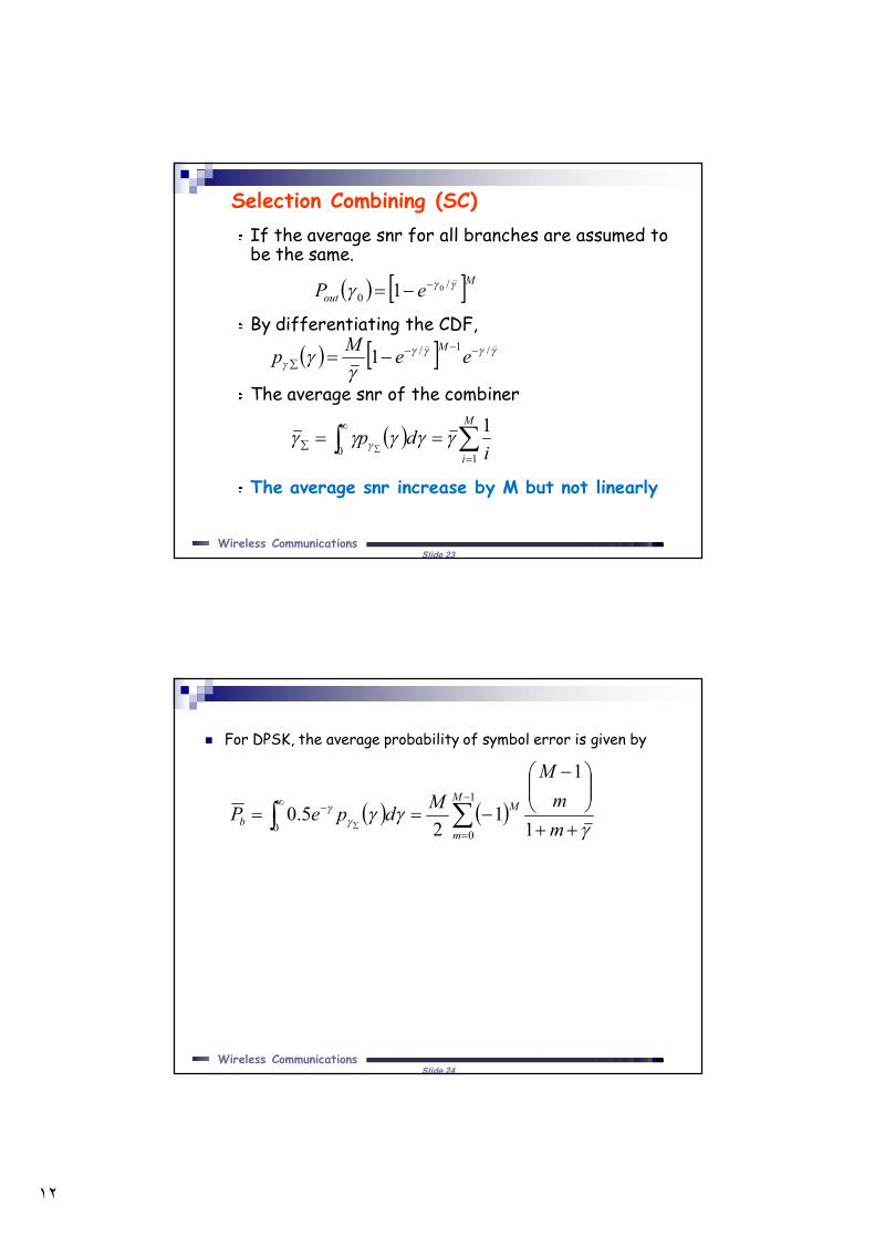
If the average snr for all branches are assumed to be the same.
By differentiating the CDF,
The average snr of the combiner
The average snr increase by M but not linearly
Selection Combining (SC)
Mout eP /0
01
M
i idp
10
1
/1/1 eeMp M
Slide 24Wireless Communications
For DPSK, the average probability of symbol error is given by
1
00 1
1
12
5.0M
m
Mb m
mM
MdpeP
١٣
Slide 25Wireless Communications
Example: Find the outage probability of BPSK modulation at Pb
= 10 −3 for a Rayleigh fading channel with SC diversity for M = 1 (no diversity),M = 2, and M = 3. Assume equal branch SNRs of γ = 15 dB.
For Pb = 10 −3 , γ0 = 7 dB= 10.7 and γ0 = 101.5.
3003.020215.0
11466.01 /
00
MM
MeP M
out
Slide 26Wireless Communications
Outage Probability of Selection Combining in Rayleigh Fading
١٤
Slide 27Wireless Communications
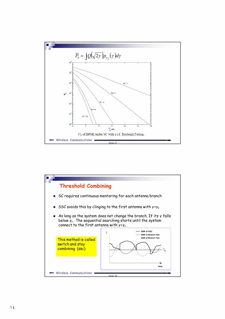
dpQPb 2
Slide 28Wireless Communications
SC requires continuous mentoring for each antenna branch
SSC avoids this by clinging to the first antenna with γ >γt.
As long as the system does not change the branch. If its γ falls below γt . The sequential searching starts until the system connect to the first antenna with γ >γt .
Threshold Combining
This method is calledswitch and stay combining (ssc)
١٥
Slide 29Wireless Communications
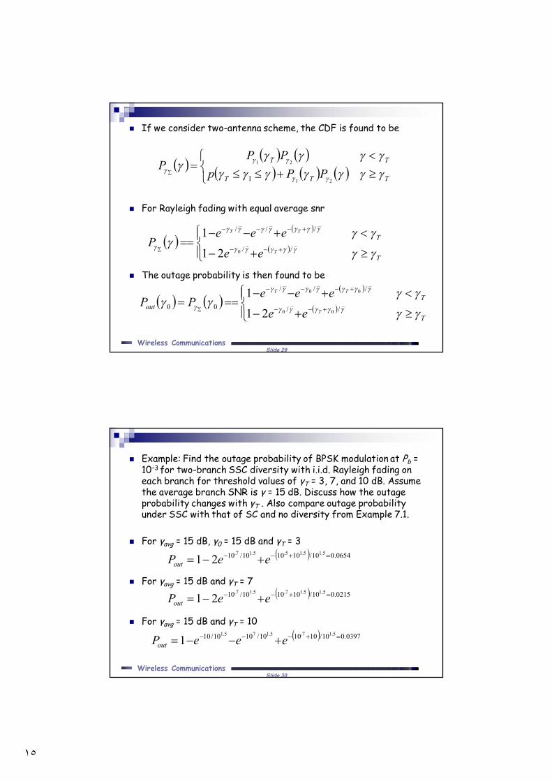
If we consider two-antenna scheme, the CDF is found to be
For Rayleigh fading with equal average snr
The outage probability is then found to be
TTT
TT
PPpPP
P
21
21
1
T
T
T
TT
ee
eeeP
//
///
021
1
T
Tout
T
TT
eeeee
PP
//
///
0000
00
21
1
Slide 30Wireless Communications
Example: Find the outage probability of BPSK modulation at Pb = 10−3 for two-branch SSC diversity with i.i.d. Rayleigh fading on each branch for threshold values of γT = 3, 7, and 10 dB. Assume the average branch SNR is γ = 15 dB. Discuss how the outage probability changes with γT . Also compare outage probability under SSC with that of SC and no diversity from Example 7.1.
For γavg = 15 dB, γ0 = 15 dB and γT = 3
For γavg = 15 dB and γT = 7
For γavg = 15 dB and γT = 10
0654.010/101010/10 5.15.15.5.17.
21 eePout
0215.010/101010/10 5.15.17.5.17.
21 eePout
0397.010/101010/1010/10 5.17.5.175.1
1 eeePout
١٦
Slide 31Wireless Communications
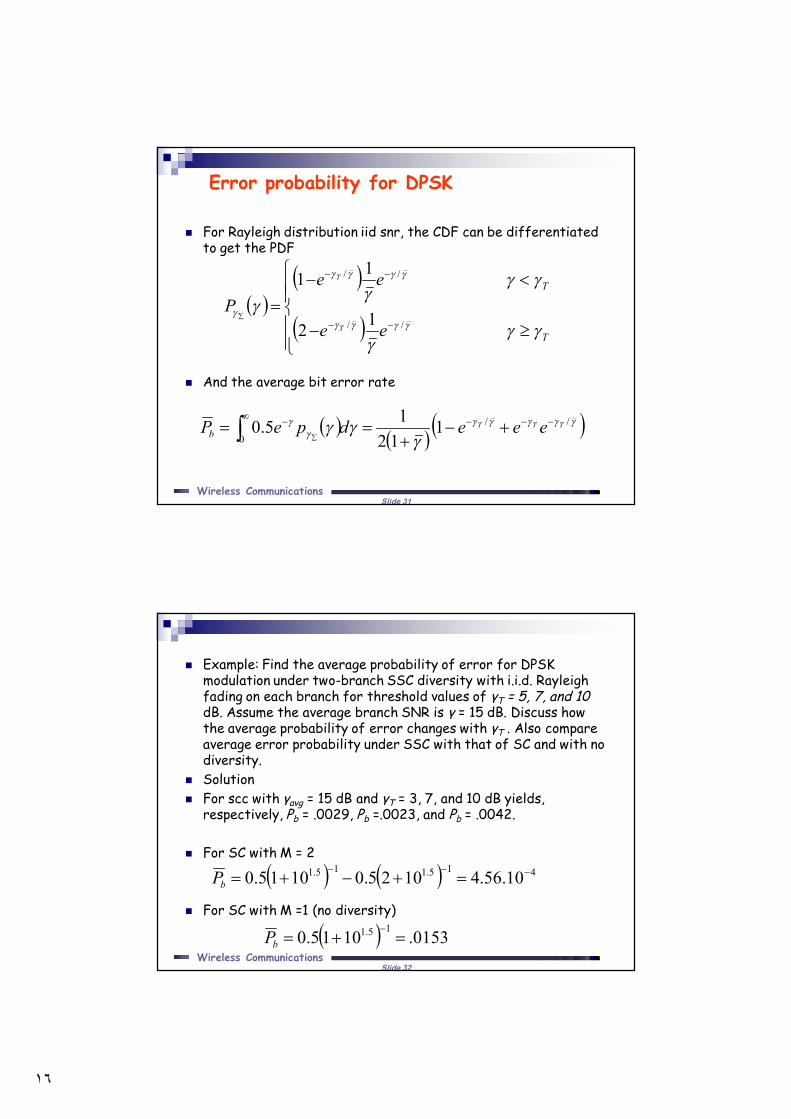
For Rayleigh distribution iid snr, the CDF can be differentiated to get the PDF
And the average bit error rate
Error probability for DPSK
T
T
ee
eeP
T
T
//
//
12
11
//
01
1215.0 TTT eeedpePb
Slide 32Wireless Communications
Example: Find the average probability of error for DPSK modulation under two-branch SSC diversity with i.i.d. Rayleigh fading on each branch for threshold values of γT = 5, 7, and 10 dB. Assume the average branch SNR is γ = 15 dB. Discuss how the average probability of error changes with γT . Also compare average error probability under SSC with that of SC and with no diversity.
Solution For scc with γavg = 15 dB and γT = 3, 7, and 10 dB yields,
respectively, Pb = .0029, Pb =.0023, and Pb = .0042.
For SC with M = 2
For SC with M =1 (no diversity)
415.115.1 10.56.41025.01015.0 bP
0153.1015.0 15.1
bP
١٧
Slide 33Wireless Communications
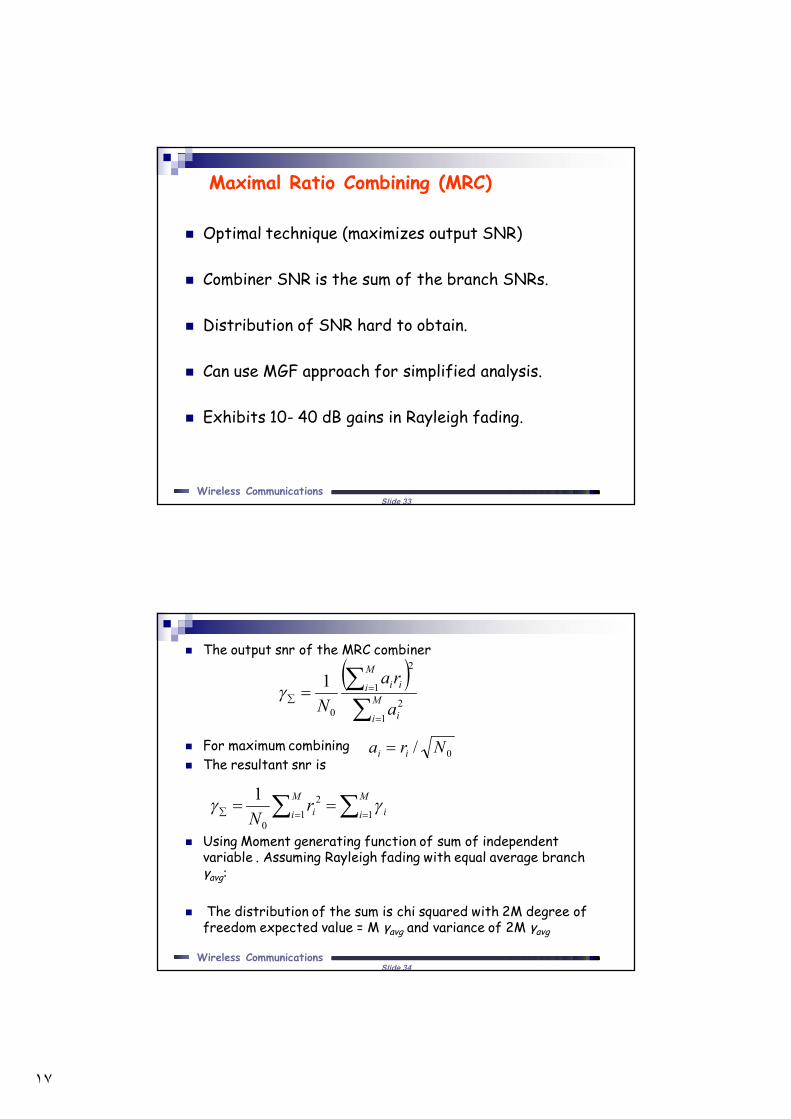
Optimal technique (maximizes output SNR)
Combiner SNR is the sum of the branch SNRs.
Distribution of SNR hard to obtain.
Can use MGF approach for simplified analysis.
Exhibits 10- 40 dB gains in Rayleigh fading.
Maximal Ratio Combining (MRC)
Slide 34Wireless Communications
The output snr of the MRC combiner
For maximum combining The resultant snr is
Using Moment generating function of sum of independent variable . Assuming Rayleigh fading with equal average branch γavg:
The distribution of the sum is chi squared with 2M degree of freedom expected value = M γavg and variance of 2M γavg
M
i i
M
i ii
a
raN
12
2
1
0
1
0/ Nra ii
M
i iM
i irN 112
0
1
١٨
Slide 35Wireless Communications
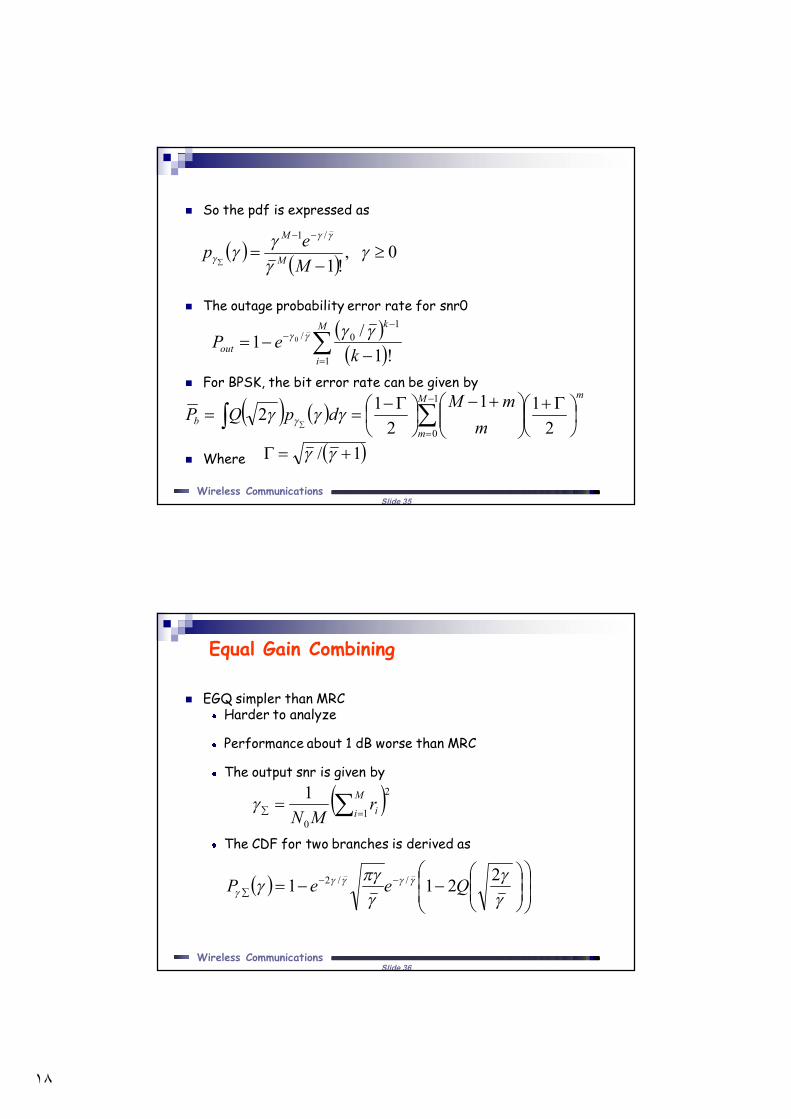
So the pdf is expressed as
The outage probability error rate for snr0
For BPSK, the bit error rate can be given by
Where
mM
mb m
mMdpQP
2
112
121
0
1/
M
i
k
out keP
1
10/
!1/1 0
0,!1
/1
Mep M
M
Slide 36Wireless Communications
EGQ simpler than MRCHarder to analyze
Performance about 1 dB worse than MRC
The output snr is given by
The CDF for two branches is derived as
Equal Gain Combining
21
0
1 M
i irMN
2211 //2 QeeP
١٩
Slide 37Wireless Communications
The resulting outage probability
By differentiating the CDF we get the pdf
And finally the probability error for BPSK is
0/0/2
02211 0 QeePout
2211
411 //2 Qeep
2
11115.02
dpQPb
Slide 38Wireless Communications
Example: Compare the average probability of bit error of BPSK under MRC and EGC two-branch diversity with i.i.d. Rayleigh fading with average SNR of 10 dB on each branch.
For MRC
For EGC
3
2
10.6.111/1022
11/101
bP
32
10.07.2111115.0
bP
٢٠
Slide 39Wireless Communications
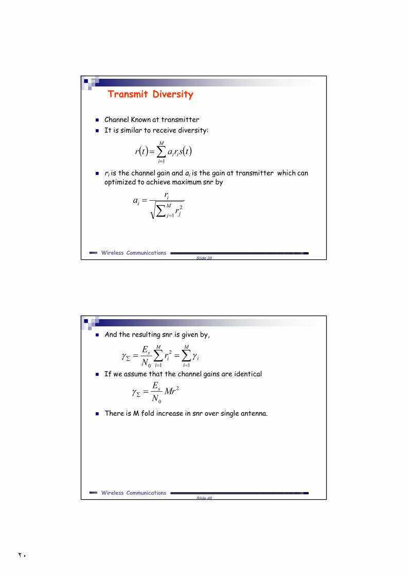
Channel Known at transmitter It is similar to receive diversity:
ri is the channel gain and ai is the gain at transmitter which can optimized to achieve maximum snr by
Transmit Diversity
M
iii tsratr
1
M
j j
ii
r
ra1
2
Slide 40Wireless Communications
And the resulting snr is given by,
If we assume that the channel gains are identical
There is M fold increase in snr over single antenna.
M
i
M
iii
s rNE
1 1
2
0
2
0
MrNEs
٢١
Slide 41Wireless Communications
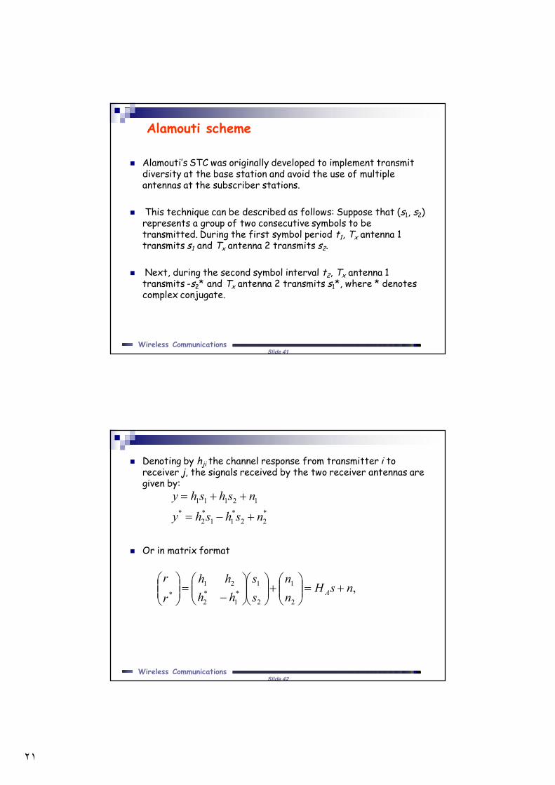
Alamouti’s STC was originally developed to implement transmit diversity at the base station and avoid the use of multiple antennas at the subscriber stations.
This technique can be described as follows: Suppose that (s1, s2) represents a group of two consecutive symbols to be transmitted. During the first symbol period t1, Tx antenna 1 transmits s1 and Tx antenna 2 transmits s2.
Next, during the second symbol interval t2, Tx antenna 1 transmits -s2* and Tx antenna 2 transmits s1*, where * denotes complex conjugate.
Alamouti scheme
Slide 42Wireless Communications
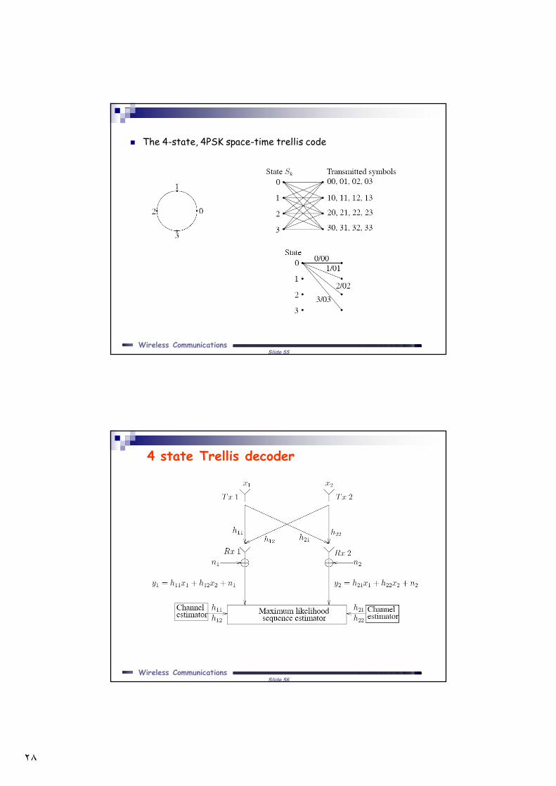
Denoting by hji the channel response from transmitter i to receiver j, the signals received by the two receiver antennas are given by:
Or in matrix format
*22
*11
*2
*12111
nshshynshshy
,2
1
2
1*1
*2
21*
nsHnn
ss
hhhh
rr
A
٢٢
Slide 43Wireless Communications
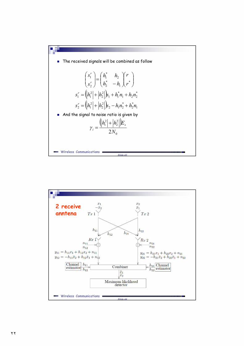
The received signals will be combined as follow
And the signal to noise ratio is given by
*
1*2
2*1
2
1
rr
hhhh
ssr
r
1
*2
*212
22
212
*221
*11
22
211
nhnhshhs
nhnhshhsr
r
0
22
21
2NEhh s
i
Slide 44Wireless Communications
2 receive anntena
٢٣
Slide 45Wireless Communications
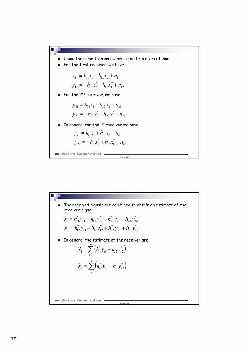
Using the same transmit scheme for 1 receive antenna For the first receiver, we have
For the 2nd receiver, we have
In general for the ith receiver we have
12*112
*21112
1121211111
nxhxhynxhxhy
22*122
*22122
2122212121
nxhxhynxhxhy
2*12
*2122
122111
iii
iiii
nxhxhynxhxhy
Slide 46Wireless Communications
The received signals are combined to obtain an estimate of the received signal
In general the estimate at the receiver are
*222121
*22
*121111
*122
*222221
*21
*121211
*111
~~
yhyhyhyhxyhyhyhyhx
q
iiiii
q
iiiii
yhyhx
yhyhx
1
*211
*22
1
*221
*11
~
~
٢٤
Slide 47Wireless Communications
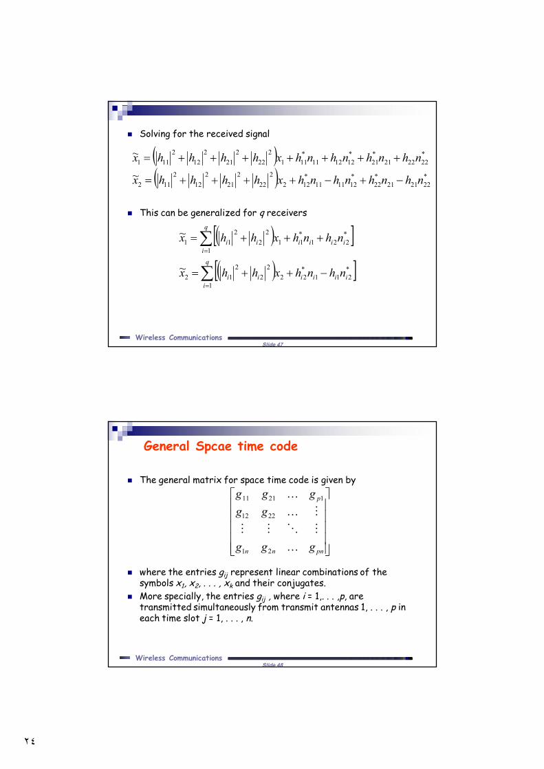
Solving for the received signal
This can be generalized for q receivers
*
222121*22
*121111
*122
222
221
212
2112
*222221
*21
*121211
*111
222
221
212
2111
~
~
nhnhnhnhxhhhhx
nhnhnhnhxhhhhx
q
iiiiiii
q
iiiiiii
nhnhxhhx
nhnhxhhx
1
*211
*22
22
212
1
*221
*11
22
211
~
~
Slide 48Wireless Communications
The general matrix for space time code is given by
where the entries gij represent linear combinations of the symbols x1, x2, . . . , xk and their conjugates.
More specially, the entries gij , where i = 1,. . . ,p, are transmitted simultaneously from transmit antennas 1, . . . , p in each time slot j = 1, . . . , n.
General Spcae time code
pnnn
p
ggg
ggggg
21
2212
12111
٢٥
Slide 49Wireless Communications
For example, in time slot j = 2, signals g12, g22, . . . , gp2 are transmitted simultaneously from transmit antennas Tx1, Tx2, . . . , Txp
The code rate of space time code is given by R = k/N
Slide 50Wireless Communications
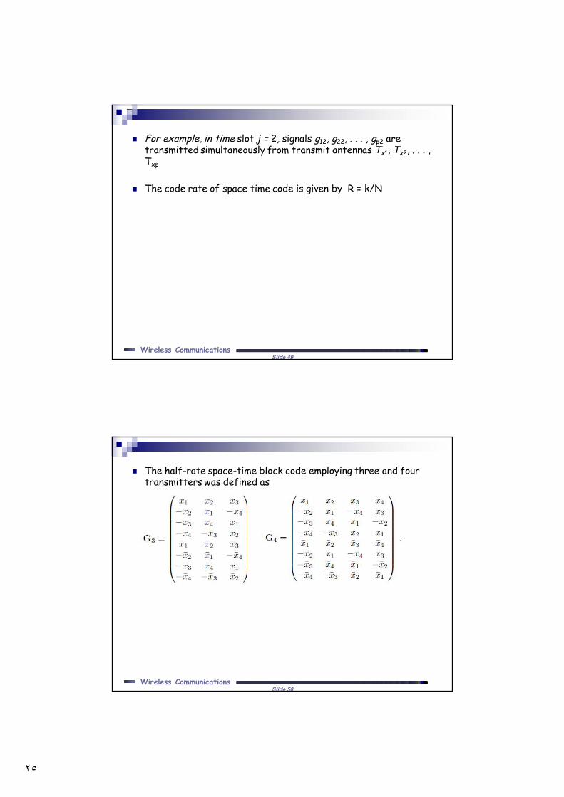
The half-rate space-time block code employing three and four transmitters was defined as
٢٦
Slide 51Wireless Communications
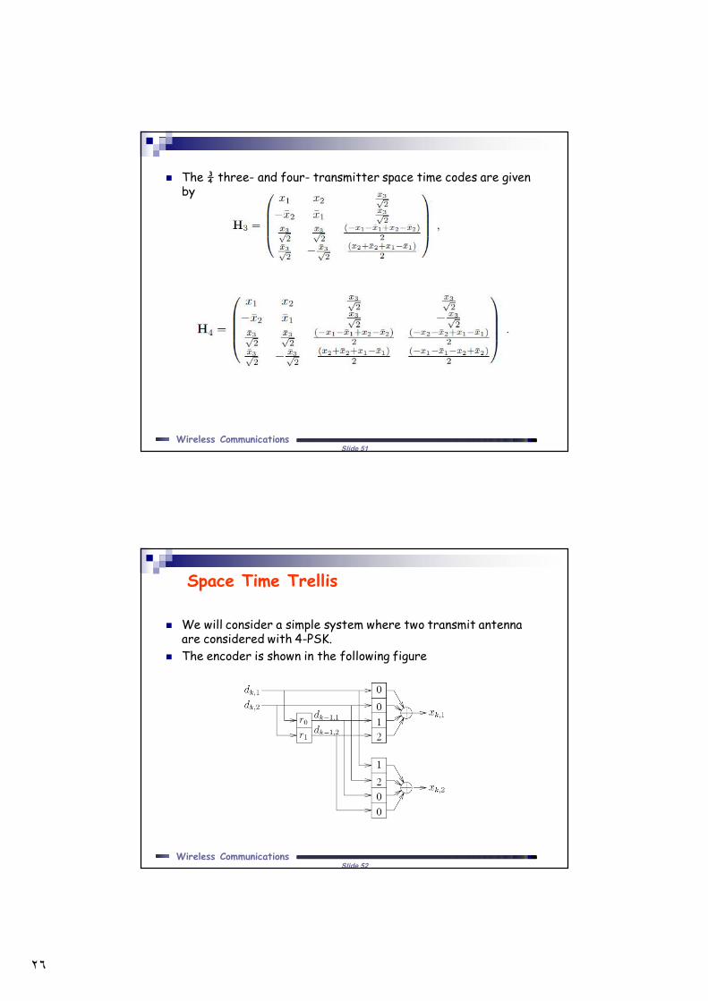
The ¾ three- and four- transmitter space time codes are given by
Slide 52Wireless Communications
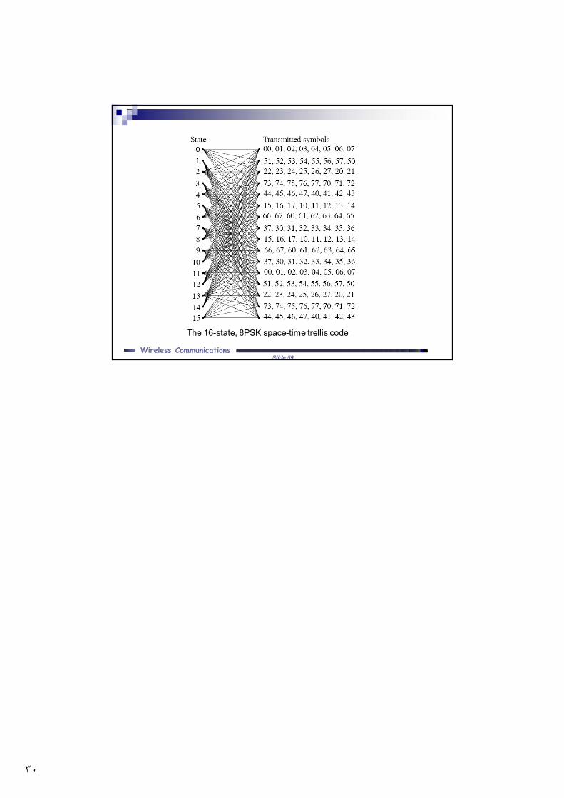
We will consider a simple system where two transmit antenna are considered with 4-PSK.
The encoder is shown in the following figure
Space Time Trellis
٢٧
Slide 53Wireless Communications
The output symbols at time instant k are given by:
r1r0 are shift register which is usually initialized by 00. Example: consider 0111000
2,11,12,1,2,
2,11,12,1,1,
.0.02.1.2.10.0
kkkkk
kkkkk
ddddxddddx
Slide 54Wireless Communications
The output symbols at time instant k are given by: