Division of Engineering and Applied Sciences DIMACS-04 Iterative Timing Recovery Aleksandar Kavčić...

Division of Engineering and Applied Sciences

DIMACS-04

Iterative Timing Recovery

Aleksandar Kavčić


Harvard University

based on a tutorial by

Barry, Kavčić, McLaughlin, Nayak & Zeng

And on research by

Motwani and Kavčić


slide 2

Outline

• Motivation• Timing model• Conventional timing recovery• Simple iterative timing recovery• Joint timing and intersymbol interference trellis• Soft decision algorithm• Performance results• Conclusion• Future challenge: capacity of channels with

synchronization error


slide 3

Motivation

• In most communications (decoding) scenarios, we assume perfect timing recovery

• This assumption breaks down, particularly at low signal-to-noise ratios (SNRs)

• But, turbo-like codes work exactly at these SNRs

• Need to take timing uncertainty into account


slide 4

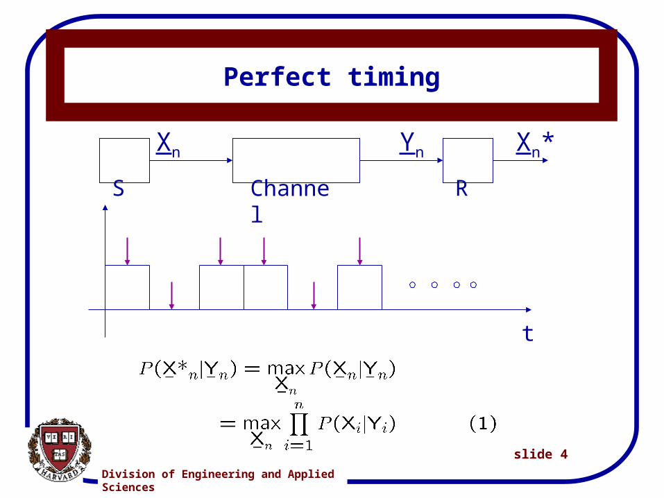
t

ChannelXn Yn S R

Xn*

Perfect timing


slide 5

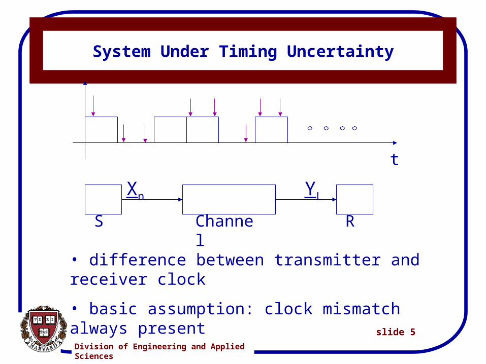
System Under Timing Uncertainty

t

ChannelXn YL S R

• difference between transmitter and receiver clock

• basic assumption: clock mismatch always present


slide 6

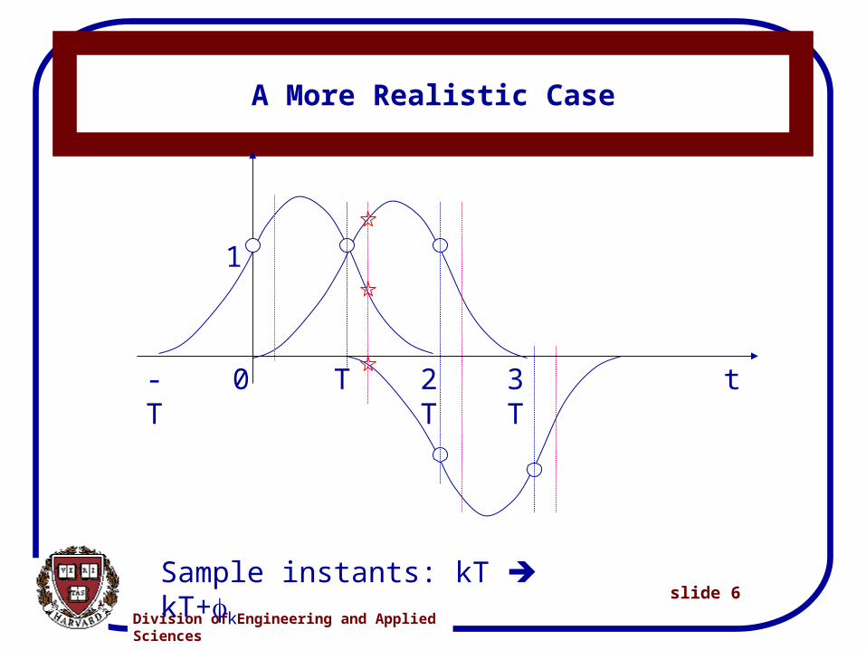
A More Realistic Case

0-T T 2T 3T t

1

Sample instants: kT kT+k


slide 7

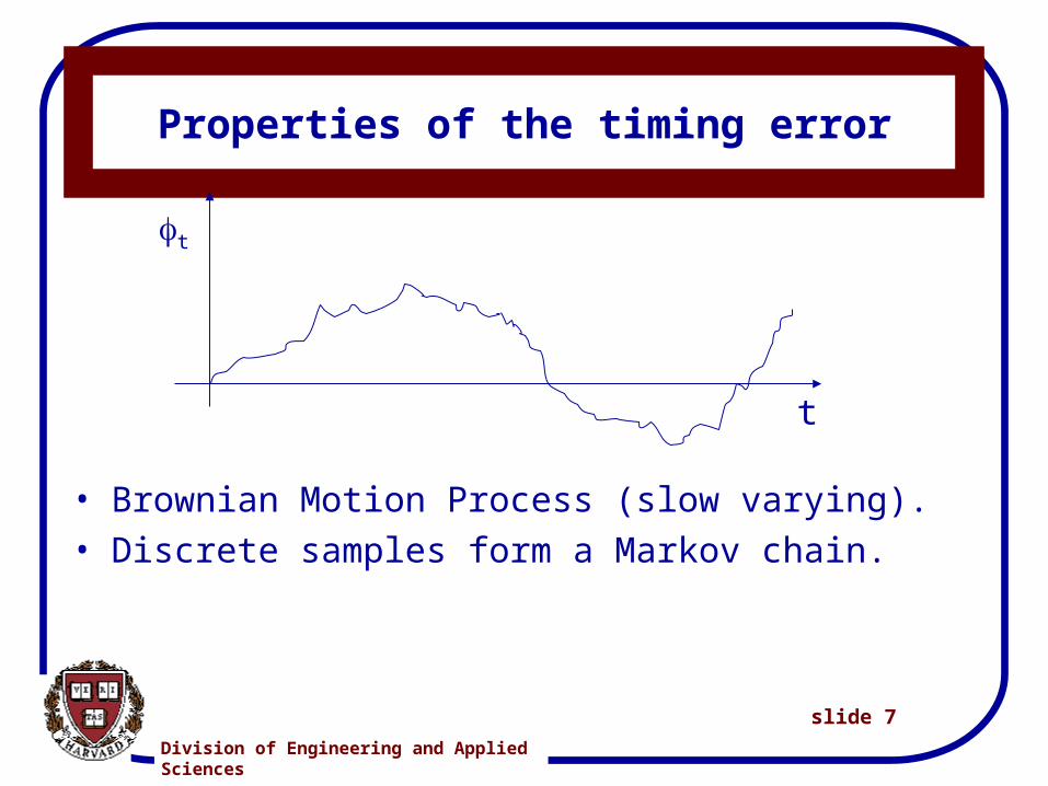
Properties of the timing error

• Brownian Motion Process (slow varying).

• Discrete samples form a Markov chain.

t

t


slide 8

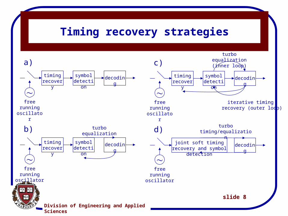
Timing recovery strategies

timingrecovery

symboldetection

decoding

timingrecovery

symboldetection

decoding

free runningoscillator


turbo equalization

timingrecovery

symboldetection

decoding

joint soft timing recovery and symbol detection

decoding



turbo timing/equalization

turbo equalization(inner loop)

iterative timing recovery (outer loop)

a)

b)

c)

d)


slide 9

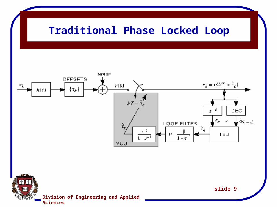
Traditional Phase Locked Loop


slide 10

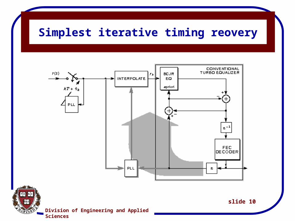
Simplest iterative timing reovery


slide 11

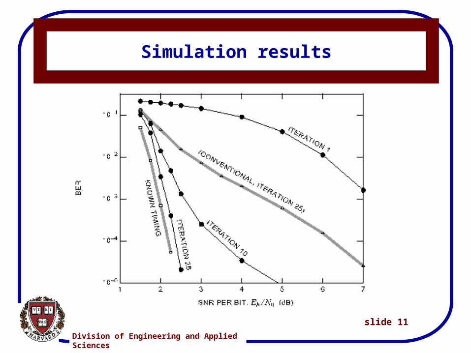
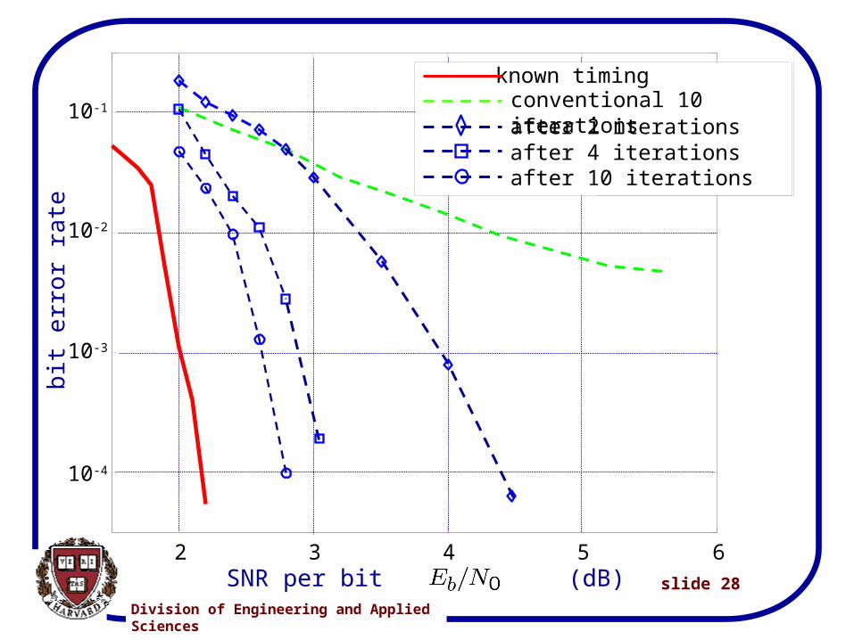
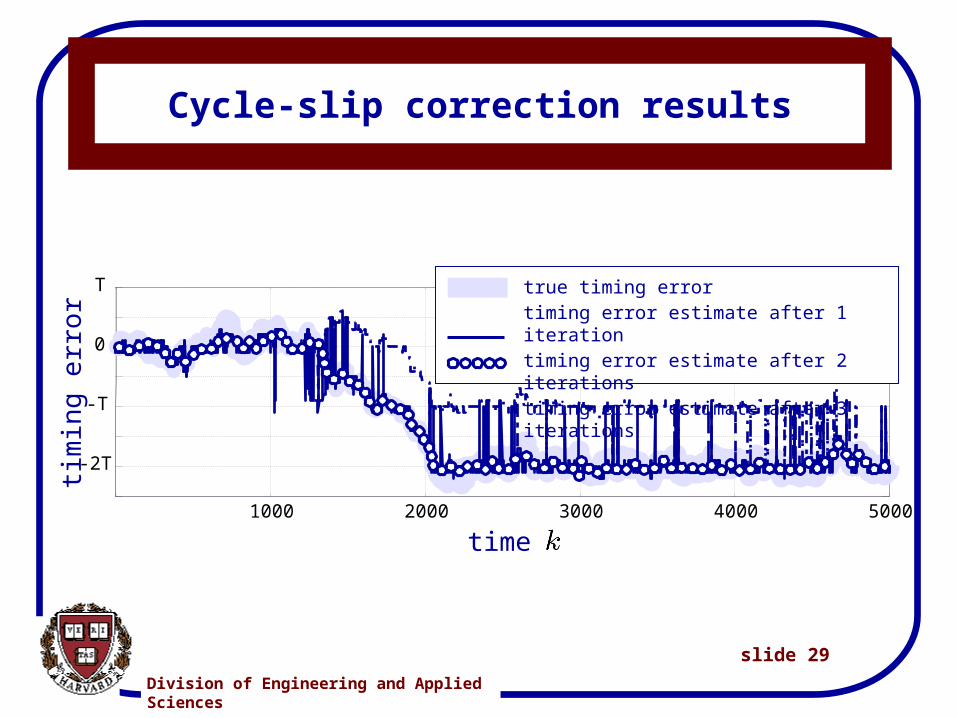
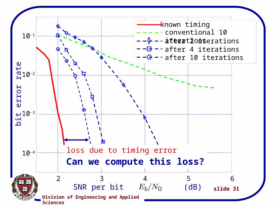
Simulation results


slide 12

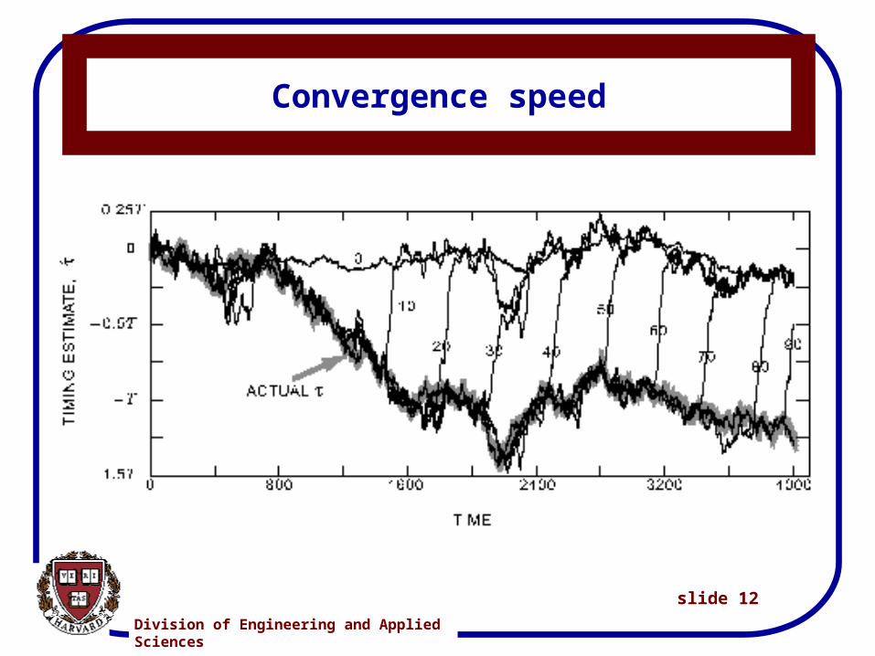
Convergence speed


slide 13

Strategy to solve the problem

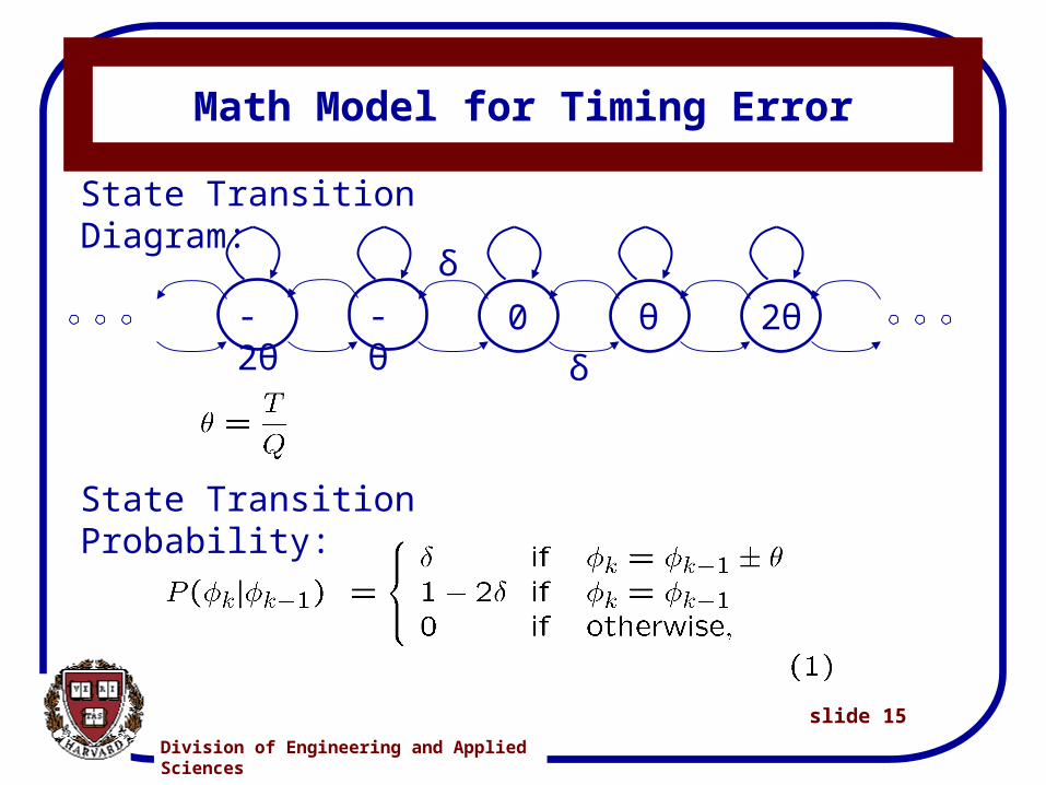
1. Set up math model for timing error (Markov).

2. Build separate stationary trellis to characterize the channel and source.

3. Form a full trellis.

4. Derive an algorithm to perform the Maximum a posteriori probability (MAP) estimation of the timing offset and the input bits


slide 14

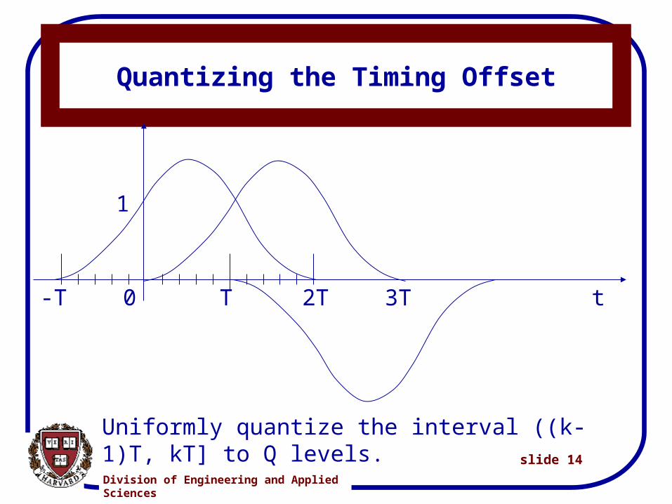
Quantizing the Timing Offset

Uniformly quantize the interval ((k-1)T, kT] to Q levels.

0-T T 2T 3T t

1


slide 15

Math Model for Timing Error

State Transition Diagram:

State Transition Probability:

0 θ 2θ-2θ -θ

δ

δ


slide 16

States for Timing Error

0-T T 2T 3T t

1

Semi-open segment : ((k-1)T, kT]:

Q 1-sample states: 1i i=1, 2, …, Q

1 deletion states: 0

1 2-sample state: 2


slide 17

Example: timing error realization

k

k10 2 3

4 5 6 7 8 9 10 11 12 13 14 150

T/Q

-T/Q

-2T/Q

-3T/Q

-4T/Q

-5T/Q = -T

Q = 5

0 T 2T 3T 4T 5T 6T 7T 8T 9T 10T

0-0 3T- 32T- 2 5T- 54T- 4T- 1 6T- 6 7T- 7 8T- 8 9T- 9

t

0thinterval

1stinterval

2ndinterval

3rdinterval

4thinterval

5thinterval

8thinterval

6thinterval

7thinterval

10thinterval

9thinterval

15 0 0215 14 14 15 11 11 12

0

11

12

13

14

15

2


slide 19

Single trellis section

0

11

12

13

14

15

2

0

11

12

13

14

15

2


slide 20

Source Model

Second order Markov chain

-1, -1 -1, -1

-1, -1, 1

1, -1

1, 1

-1, -1 -1, -1

-1, -1, 1

1, -1

1, 1

-1, -1 -1, -1

-1, -1, 1

1, -1

1, 1

-1, -1 -1, -1

-1, -1, 1

1, -1

1, 1


slide 21

Full Trellis

Full states set:

Total number of states at each time interval:

Trellis length = n (block length). (note that each branch may have different number of outputs).

(-1,-1)

(-1,1)

(1,-1)

(1,1)

(-1,-1)(-1,1)

(1,-1)

(1,1)

b) ISI trellis

(-1,-1,0)

(-1,-1,11)

(-1,1,11)

(1,-1,11)

(1,1,11)

(1,-1,2)

(1,1,2)

(-1,-1,12)

(-1,-1,0)

(-1,-1,11)

(-1,1,11)

(1,-1,11)

(1,1,11)

(1,-1,2)

(1,1,2)

(-1,1,12)

……

…

……

…

……

…c) joint ISI-timing trellis

-2T 0-T T 2T 3T

1

0

h(t)

3T/5-2T/5 8T/5

a) pulse example

Joint Trellis Example


slide 23

Soft-Output Detector


slide 24

Definition of Some Functions

Notation:

Definition:


slide 25

Calculation of the Soft-outputs


slide 26

Recursion of α(t,m,i)


slide 27

Recursion of β(t,m,i)


slide 28

2 3 4 5 6

10-4

10-3

10-2

10-1

known timing

after 10 iterations

after 2 iterations conventional 10 iterations

after 4 iterations

bit

err

or r

ate

SNR per bit (dB)


slide 29

Cycle-slip correction results

1000 2000 3000 4000 5000

-2T

-T

0

T true timing errortiming error estimate after 1 iterationtiming error estimate after 2 iterationstiming error estimate after 3 iterations

time

timin

g e

rro

r


slide 30

Conclusion

• Conventional timing recovery fails at low SNR because it ignores the error-correction code.

• Iterative timing recovery exploits the power of the code.

• Performance close to perfect timing recovery

• Only marginal increase in complexity compared to system that uses conventional turbo equalization/decoding


slide 31

2 3 4 5 6

10-4

10-3

10-2

10-1

known timing

after 10 iterations

after 2 iterations conventional 10 iterations

after 4 iterations

bit

err

or r

ate

SNR per bit (dB)

loss due to timing error

Can we compute this loss?


slide 32

Open Problems

• Information Theory for channels with synchronization error:– Capacity– Capacity achieving distribution– Capacity achieving codes


slide 33

Deletion channels

• Transmitted sequence x1, x2, x3, ….

– Xk { 0, 1 }

• Received sequence y1, y2, y3, ….– Sequence y is a subsequence of sequence x

• Symbol xk is deleted with probability


slide 34

Deletion channels

• Some results:– Ulmann 1968, upper bounds on the capacities of

deletion channels– Diggavi&Grossglauser 2002, analytic lower bounds on

capacities of deletion channels– Mitzenmacher 2004, tighter analytic lower bounds


slide 35


slide 36

Numerical capacity computation methods


slide 37

Received symbols per transmitted symbol

Let K(m) denote the number of received symbols per m transmitted symbols

K(m) is a random variable

Asymptotically, we have A received symbols per transmitted symbol

For the deletion channel,


slide 38

Capacity per transmitted symbol

upper boundcompute


slide 39

Markov sources

0

1

0

1

P00/0

P11/1

P01/1 P10/0

st-1 st

Prob/xt

0

1

0

1

Q00/0

Q11/1

Q01/1 Q10/0

st-1 st

Prob/yt

If X is a first-order Markov source (transition matrix P), then Y is also a first-order Markov source (transition matrix Q)


slide 40

Trellis for Y | X

011

02

(1-)/1

s0 s1

Prob/y1

s2

(1-)/0

(1-)2/0

(1-)3/1

03

14

02

03

14

15

(1-)/0

(1-)/0

(1-)2/1

(1-)/0

(1-)/1

(1-)/1

(1-)/1

Prob/y2

… ……

…

…

…

Run a reduced-stateBCJR algorithm on tis trellisto upper-bound H(Y|X)


slide 41


slide 42

Future research

• Upper bounds for insertion/deletion channels?

• Channels with non-integer timing error?

• Codes?

(long run-lengths are favored in deletion channels)

Date post:	21-Dec-2015
Category:	Documents
View:	219 times
Download:	3 times

Division of Engineering and Applied Sciences DIMACS-04 Iterative Timing Recovery Aleksandar Kavčić...

Documents