43
DNA Microarrays Patrick Schmid CSE 497 Spring 2004
| Date post: | 23-Dec-2015 |
| Category: |
Documents |
| Upload: | griffin-heath |
| View: | 218 times |
| Download: | 0 times |
DNA Microarrays
Patrick Schmid
CSE 497
Spring 2004
Patrick Schmid 2
What is a DNA Microarray?
Also known as DNA Chip Allows simultaneous measurement of the
level of transcription for every gene in a genome (gene expression)
Transcription? Process of copying of DNA into messenger RNA
(mRNA) Environment dependant!
Microarray detects mRNA, or rather the more stable cDNA
Patrick Schmid 3
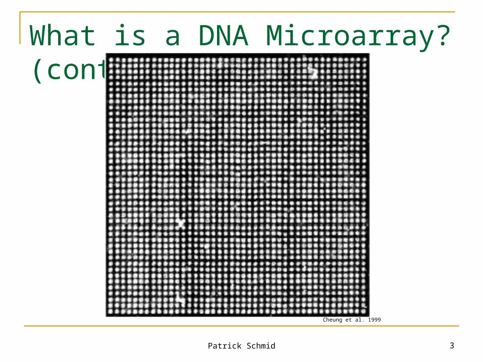
What is a DNA Microarray? (cont.)
Cheung et al. 1999
Patrick Schmid 4
How do we manufacture a microarray? Start with individual genes, e.g. the ~6,200
genes of the yeast genome Amplify all of them using polymerase chain
reaction (PCR) “Spot” them on a medium, e.g. an ordinary
glass microscope slide Each spot is about 100 µm in diameter Spotting is done by a robot Complex and potentially expensive task
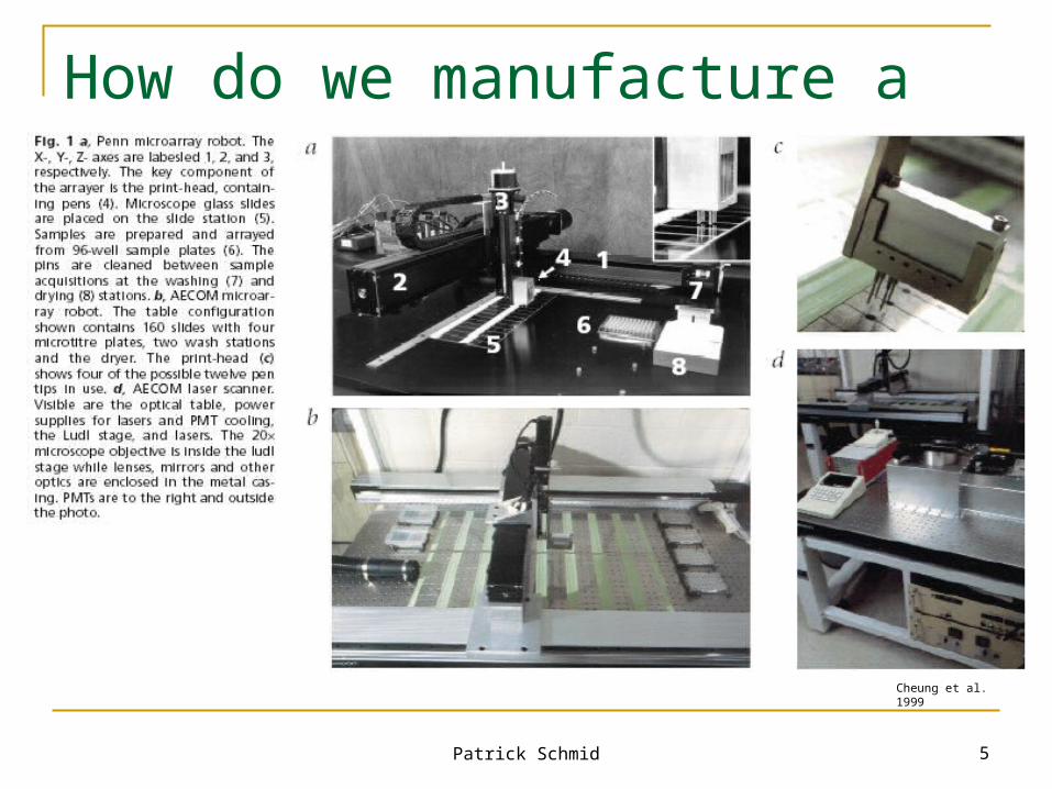
Patrick Schmid 5
How do we manufacture a microarray?
Cheung et al. 1999
Patrick Schmid 6
Example
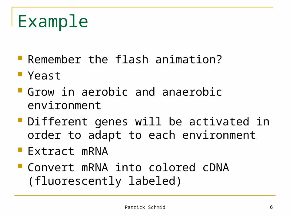
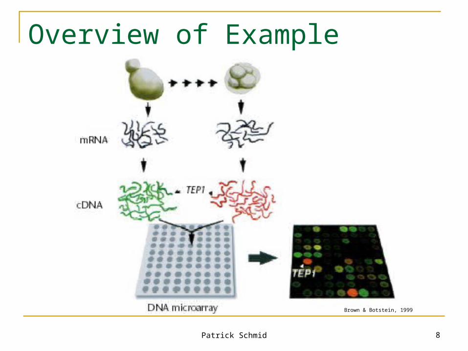
Remember the flash animation? Yeast Grow in aerobic and anaerobic environment Different genes will be activated in order to
adapt to each environment Extract mRNA Convert mRNA into colored cDNA
(fluorescently labeled)
Patrick Schmid 7
Example (cont.)
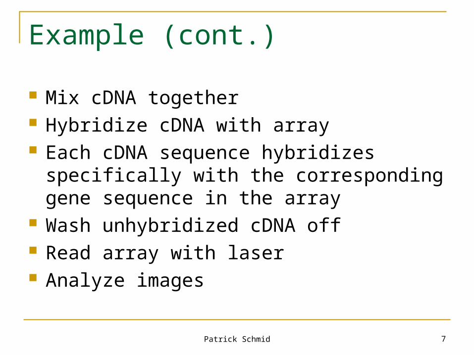
Mix cDNA together Hybridize cDNA with array Each cDNA sequence hybridizes specifically
with the corresponding gene sequence in the array
Wash unhybridized cDNA off Read array with laser Analyze images
Patrick Schmid 8
Overview of Example
Brown & Botstein, 1999
Patrick Schmid 9
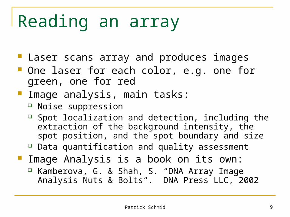
Reading an array
Laser scans array and produces images One laser for each color, e.g. one for green, one for
red Image analysis, main tasks:
Noise suppression Spot localization and detection, including the extraction of
the background intensity, the spot position, and the spot boundary and size
Data quantification and quality assessment Image Analysis is a book on its own:
Kamberova, G. & Shah, S. “DNA Array Image Analysis Nuts & Bolts“. DNA Press LLC, 2002
Patrick Schmid 10
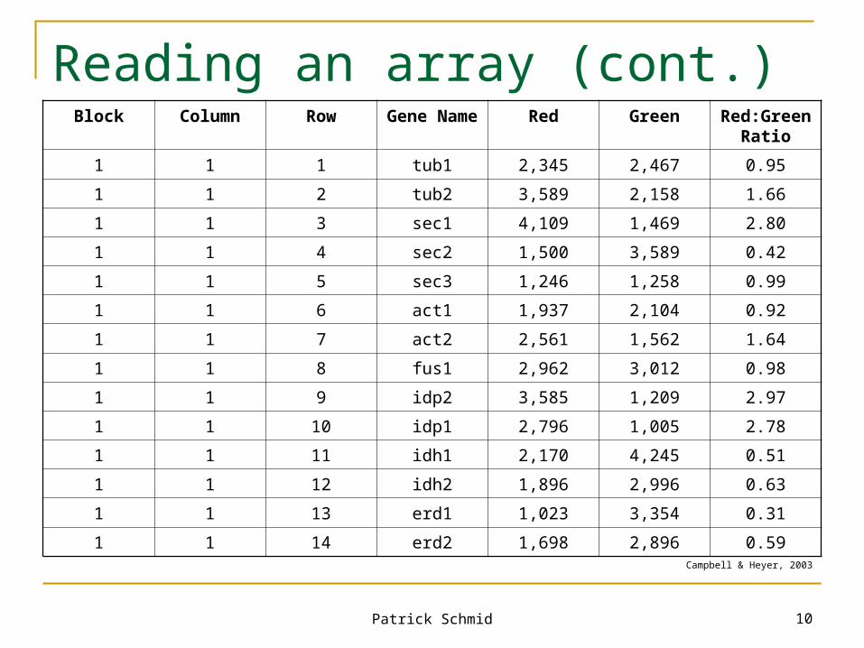
Reading an array (cont.)Block Column Row Gene Name Red Green Red:Green
Ratio
1 1 1 tub1 2,345 2,467 0.95
1 1 2 tub2 3,589 2,158 1.66
1 1 3 sec1 4,109 1,469 2.80
1 1 4 sec2 1,500 3,589 0.42
1 1 5 sec3 1,246 1,258 0.99
1 1 6 act1 1,937 2,104 0.92
1 1 7 act2 2,561 1,562 1.64
1 1 8 fus1 2,962 3,012 0.98
1 1 9 idp2 3,585 1,209 2.97
1 1 10 idp1 2,796 1,005 2.78
1 1 11 idh1 2,170 4,245 0.51
1 1 12 idh2 1,896 2,996 0.63
1 1 13 erd1 1,023 3,354 0.31
1 1 14 erd2 1,698 2,896 0.59Campbell & Heyer, 2003
Patrick Schmid 11
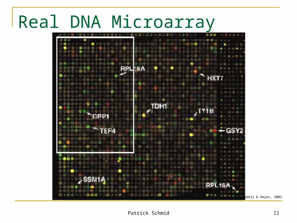
Real DNA Microarray
Campbell & Heyer, 2003
Patrick Schmid 12
Y-fold
Biologists rather deal with folds than with ratios A fold is nothing else than saying “times” We express it either as a Y-fold repression, or a
Y-fold induction It is calculated by taking the inverse of the ratio
Ratio of 0.33 = 3-fold repression Ratio of 10 = 10-fold induction
Fractional ratios can cause problems with techniques of analyzing and comparing gene expression patterns
Patrick Schmid 13
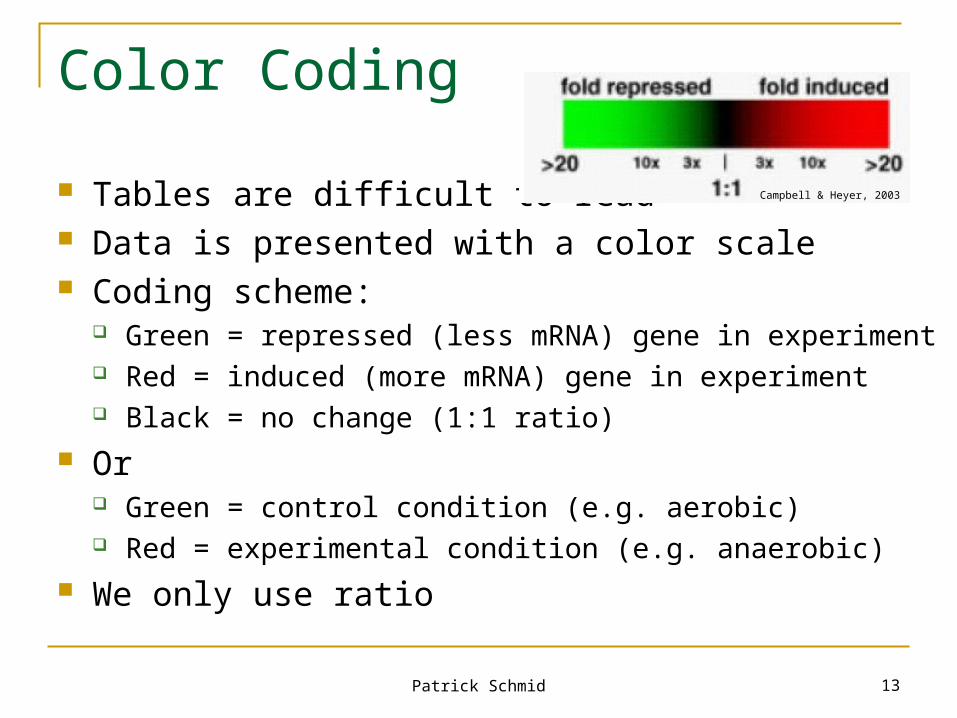
Color Coding
Tables are difficult to read Data is presented with a color scale Coding scheme:
Green = repressed (less mRNA) gene in experiment Red = induced (more mRNA) gene in experiment Black = no change (1:1 ratio)
Or Green = control condition (e.g. aerobic) Red = experimental condition (e.g. anaerobic)
We only use ratio
Campbell & Heyer, 2003
Patrick Schmid 14
Logarithmic transformation
log2 is commonly used Sometimes log10 is used Example:
log2(0.0625) = log2(1/16) = log2(1) – log2(16) = -log2(16) = -4
log2 transformations ease identification of doublings or halvings in ratios
log10 transformations ease identification of order of magnitude changes
Key attribute: equally sized induction and repression receive equal treatment visually and mathematically
Patrick Schmid 15
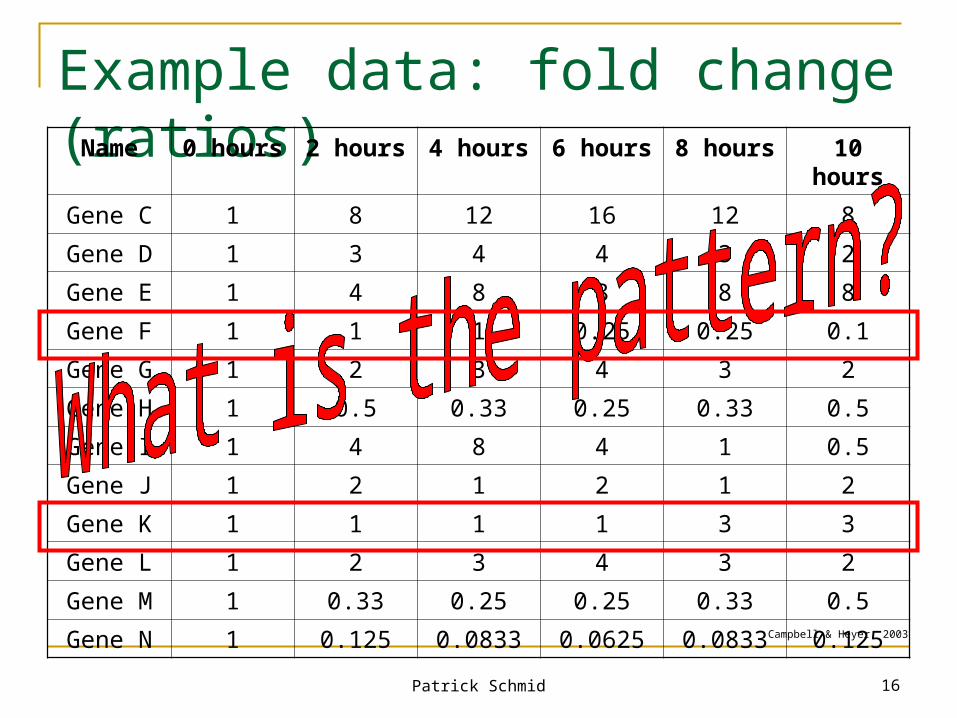
Complication: Time Series
Biologists care more about the process of adaptation than about the end result
For example, measure every 2 hours for 10 hours (depletion of oxygen)
31,000 gene expression ratios Or 6,200 different graphs with five data points each Question: Are there any genes that responded in
similar ways to the depletion of oxygen?
Patrick Schmid 16
Example data: fold change (ratios)Name 0 hours 2 hours 4 hours 6 hours 8 hours 10 hours
Gene C 1 8 12 16 12 8
Gene D 1 3 4 4 3 2
Gene E 1 4 8 8 8 8
Gene F 1 1 1 0.25 0.25 0.1
Gene G 1 2 3 4 3 2
Gene H 1 0.5 0.33 0.25 0.33 0.5
Gene I 1 4 8 4 1 0.5
Gene J 1 2 1 2 1 2
Gene K 1 1 1 1 3 3
Gene L 1 2 3 4 3 2
Gene M 1 0.33 0.25 0.25 0.33 0.5
Gene N 1 0.125 0.0833 0.0625 0.0833 0.125Campbell & Heyer, 2003
Patrick Schmid 17
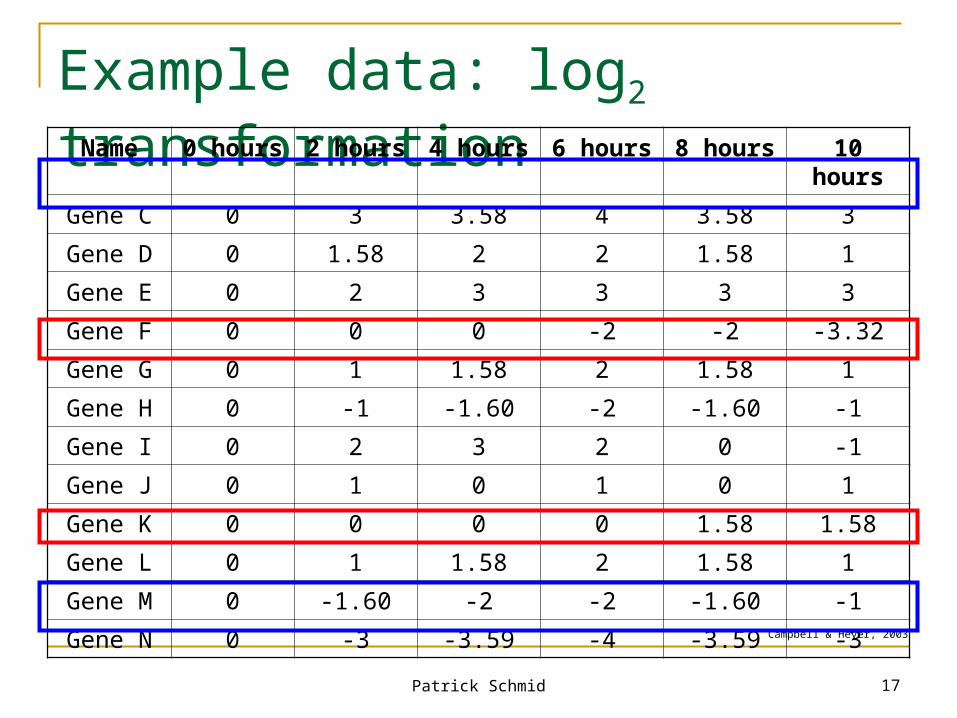
Example data: log2 transformationName 0 hours 2 hours 4 hours 6 hours 8 hours 10 hours
Gene C 0 3 3.58 4 3.58 3
Gene D 0 1.58 2 2 1.58 1
Gene E 0 2 3 3 3 3
Gene F 0 0 0 -2 -2 -3.32
Gene G 0 1 1.58 2 1.58 1
Gene H 0 -1 -1.60 -2 -1.60 -1
Gene I 0 2 3 2 0 -1
Gene J 0 1 0 1 0 1
Gene K 0 0 0 0 1.58 1.58
Gene L 0 1 1.58 2 1.58 1
Gene M 0 -1.60 -2 -2 -1.60 -1
Gene N 0 -3 -3.59 -4 -3.59 -3Campbell & Heyer, 2003
Patrick Schmid 18
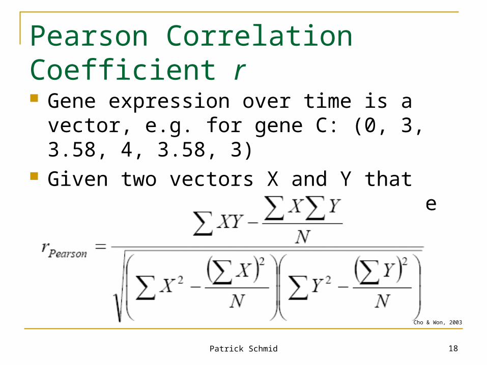
Pearson Correlation Coefficient r Gene expression over time is a vector, e.g.
for gene C: (0, 3, 3.58, 4, 3.58, 3) Given two vectors X and Y that contain N
elements, we calculate r as follows:
Cho & Won, 2003
Patrick Schmid 19
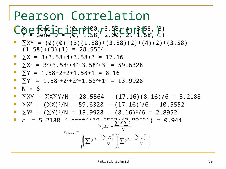
Pearson Correlation Coefficient r (cont.) X = Gene C = (0, 3.00, 3.58, 4, 3.58, 3)
Y = Gene D = (0, 1.58, 2.00, 2, 1.58, 1) ∑XY = (0)(0)+(3)(1.58)+(3.58)(2)+(4)(2)+(3.58)(1.58)+(3)(1) = 28.5564 ∑X = 3+3.58+4+3.58+3 = 17.16 ∑X2 = 32+3.582+42+3.582+32 = 59.6328 ∑Y = 1.58+2+2+1.58+1 = 8.16 ∑Y2 = 1.582+22+22+1.582+12 = 13.9928 N = 6 ∑XY – ∑X∑Y/N = 28.5564 – (17.16)(8.16)/6 = 5.2188 ∑X2 – (∑X)2/N = 59.6328 – (17.16)2/6 = 10.5552 ∑Y2 – (∑Y)2/N = 13.9928 – (8.16)2/6 = 2.8952 r = 5.2188 / sqrt((10.5552)(2.8952)) = 0.944
Patrick Schmid 20
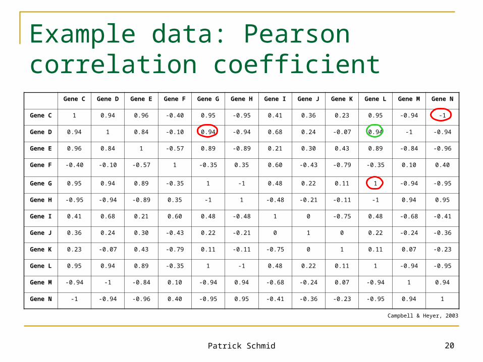
Example data: Pearson correlation coefficient
Gene C Gene D Gene E Gene F Gene G Gene H Gene I Gene J Gene K Gene L Gene M Gene N
Gene C 1 0.94 0.96 -0.40 0.95 -0.95 0.41 0.36 0.23 0.95 -0.94 -1
Gene D 0.94 1 0.84 -0.10 0.94 -0.94 0.68 0.24 -0.07 0.94 -1 -0.94
Gene E 0.96 0.84 1 -0.57 0.89 -0.89 0.21 0.30 0.43 0.89 -0.84 -0.96
Gene F -0.40 -0.10 -0.57 1 -0.35 0.35 0.60 -0.43 -0.79 -0.35 0.10 0.40
Gene G 0.95 0.94 0.89 -0.35 1 -1 0.48 0.22 0.11 1 -0.94 -0.95
Gene H -0.95 -0.94 -0.89 0.35 -1 1 -0.48 -0.21 -0.11 -1 0.94 0.95
Gene I 0.41 0.68 0.21 0.60 0.48 -0.48 1 0 -0.75 0.48 -0.68 -0.41
Gene J 0.36 0.24 0.30 -0.43 0.22 -0.21 0 1 0 0.22 -0.24 -0.36
Gene K 0.23 -0.07 0.43 -0.79 0.11 -0.11 -0.75 0 1 0.11 0.07 -0.23
Gene L 0.95 0.94 0.89 -0.35 1 -1 0.48 0.22 0.11 1 -0.94 -0.95
Gene M -0.94 -1 -0.84 0.10 -0.94 0.94 -0.68 -0.24 0.07 -0.94 1 0.94
Gene N -1 -0.94 -0.96 0.40 -0.95 0.95 -0.41 -0.36 -0.23 -0.95 0.94 1
Campbell & Heyer, 2003
Patrick Schmid 21
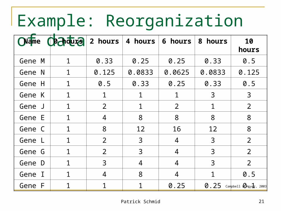
Example: Reorganization of data
Campbell & Heyer, 2003
Name 0 hours 2 hours 4 hours 6 hours 8 hours 10 hours
Gene M 1 0.33 0.25 0.25 0.33 0.5
Gene N 1 0.125 0.0833 0.0625 0.0833 0.125
Gene H 1 0.5 0.33 0.25 0.33 0.5
Gene K 1 1 1 1 3 3
Gene J 1 2 1 2 1 2
Gene E 1 4 8 8 8 8
Gene C 1 8 12 16 12 8
Gene L 1 2 3 4 3 2
Gene G 1 2 3 4 3 2
Gene D 1 3 4 4 3 2
Gene I 1 4 8 4 1 0.5
Gene F 1 1 1 0.25 0.25 0.1
Patrick Schmid 22
Clustering of example
Campbell & Heyer, 2003
Patrick Schmid 23
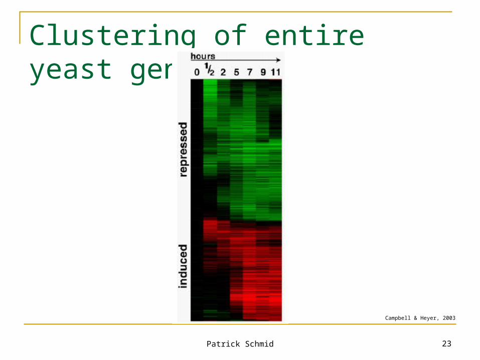
Clustering of entire yeast genome
Campbell & Heyer, 2003
Patrick Schmid 24
Hierarchical Clustering
Algorithm: First, find the two most similar genes in the entire
set of genes. Join these together into a cluster. Now join the next two most similar objects (an object can be a gene or a cluster), forming a new cluster. Add the new cluster to the list of available objects, and remove the two objects used to form the new cluster. Continue this process, joining objects in the order of their similarity to one another, until there is only one object on the list – a single cluster containing all genes.
(Campbell & Heyer, 2003)
Patrick Schmid 25
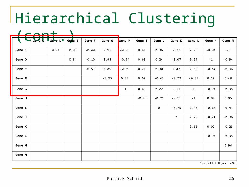
Hierarchical Clustering (cont.)Gene C Gene D Gene E Gene F Gene G Gene H Gene I Gene J Gene K Gene L Gene M Gene N
Gene C 0.94 0.96 -0.40 0.95 -0.95 0.41 0.36 0.23 0.95 -0.94 -1
Gene D 0.84 -0.10 0.94 -0.94 0.68 0.24 -0.07 0.94 -1 -0.94
Gene E -0.57 0.89 -0.89 0.21 0.30 0.43 0.89 -0.84 -0.96
Gene F -0.35 0.35 0.60 -0.43 -0.79 -0.35 0.10 0.40
Gene G -1 0.48 0.22 0.11 1 -0.94 -0.95
Gene H -0.48 -0.21 -0.11 -1 0.94 0.95
Gene I 0 -0.75 0.48 -0.68 -0.41
Gene J 0 0.22 -0.24 -0.36
Gene K 0.11 0.07 -0.23
Gene L -0.94 -0.95
Gene M 0.94
Gene N
Campbell & Heyer, 2003
Patrick Schmid 26
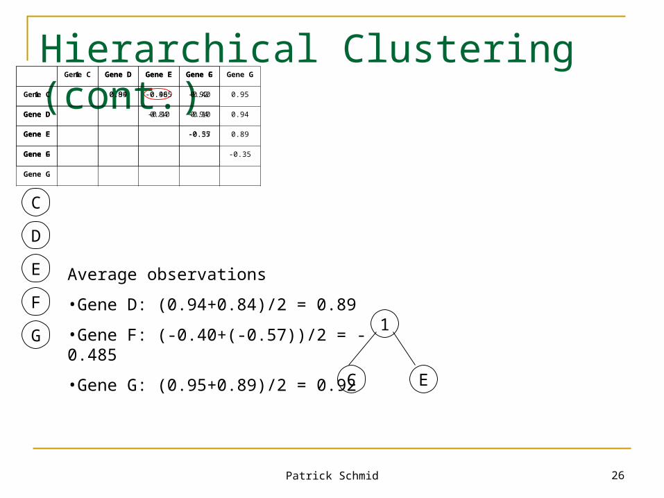
Hierarchical Clustering (cont.)
F
C
G
D
E
Gene C Gene D Gene E Gene F Gene G
Gene C 0.94 0.96 -0.40 0.95
Gene D 0.84 -0.10 0.94
Gene E -0.57 0.89
Gene F -0.35
Gene G
C E
1
1 Gene D Gene F Gene G
1 0.89 -0.485 0.92
Gene D -0.10 0.94
Gene F -0.35
Gene G
Average observations
•Gene D: (0.94+0.84)/2 = 0.89
•Gene F: (-0.40+(-0.57))/2 = -0.485
•Gene G: (0.95+0.89)/2 = 0.92
Patrick Schmid 27
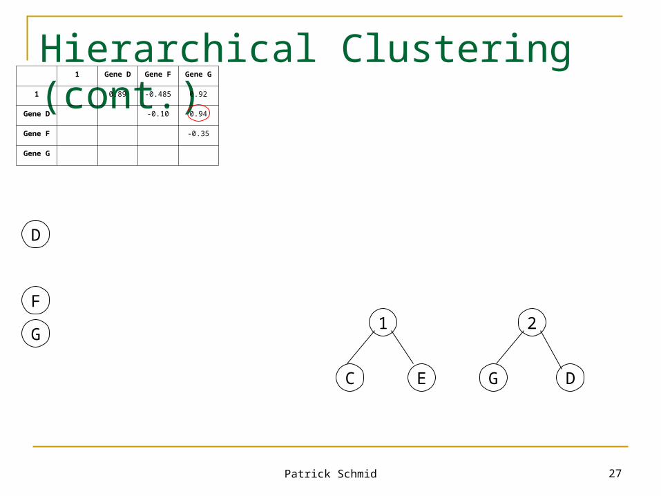
Hierarchical Clustering (cont.)
F
G
D
C E
1
1 Gene D Gene F Gene G
1 0.89 -0.485 0.92
Gene D -0.10 0.94
Gene F -0.35
Gene G
G D
2
Patrick Schmid 28
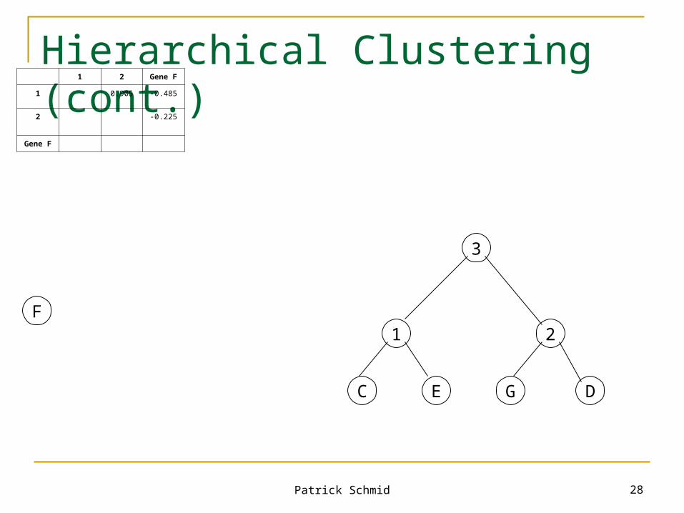
Hierarchical Clustering (cont.)
F
C E
1
G D
2
1 2 Gene F
1 0.905 -0.485
2 -0.225
Gene F
3
Patrick Schmid 29
Hierarchical Clustering (cont.)
F C E
1
G D
2
3
3 Gene F
3 -0.355
Gene F
4
F
Patrick Schmid 30
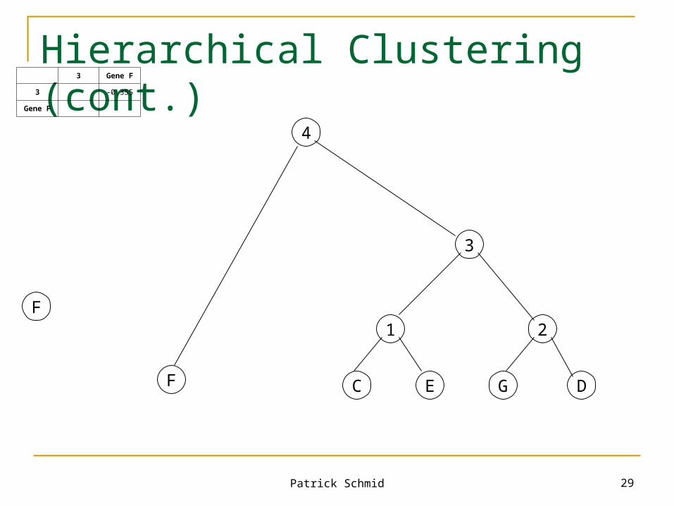
Hierarchical Clustering (cont.)
F C E
1
G D
2
3
4
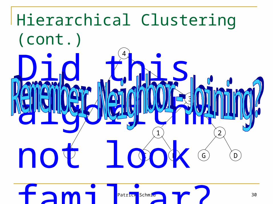
Did this algorithm not look familiar?
Patrick Schmid 31
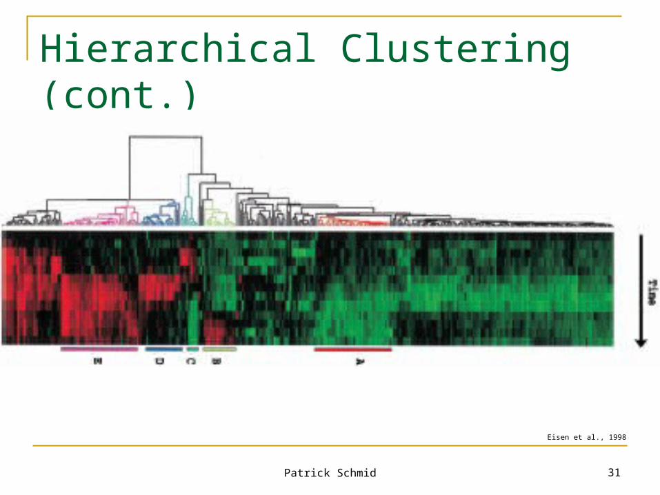
Hierarchical Clustering (cont.)
Eisen et al., 1998
Patrick Schmid 32
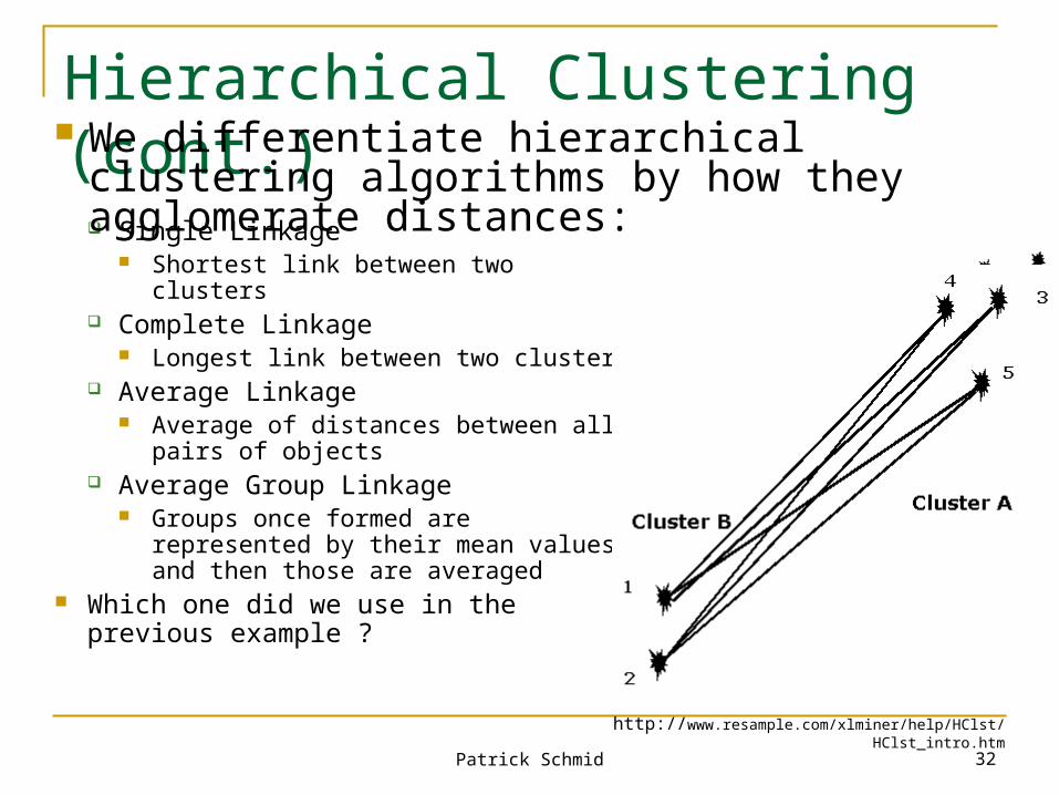
Hierarchical Clustering (cont.)
Single Linkage Shortest link between two clusters
Complete Linkage Longest link between two clusters
Average Linkage Average of distances between all
pairs of objects Average Group Linkage
Groups once formed are represented by their mean values, and then those are averaged
Which one did we use in the previous example ?
We differentiate hierarchical clustering algorithms by how they agglomerate distances:
http://www.resample.com/xlminer/help/HClst/HClst_intro.htm
Patrick Schmid 33
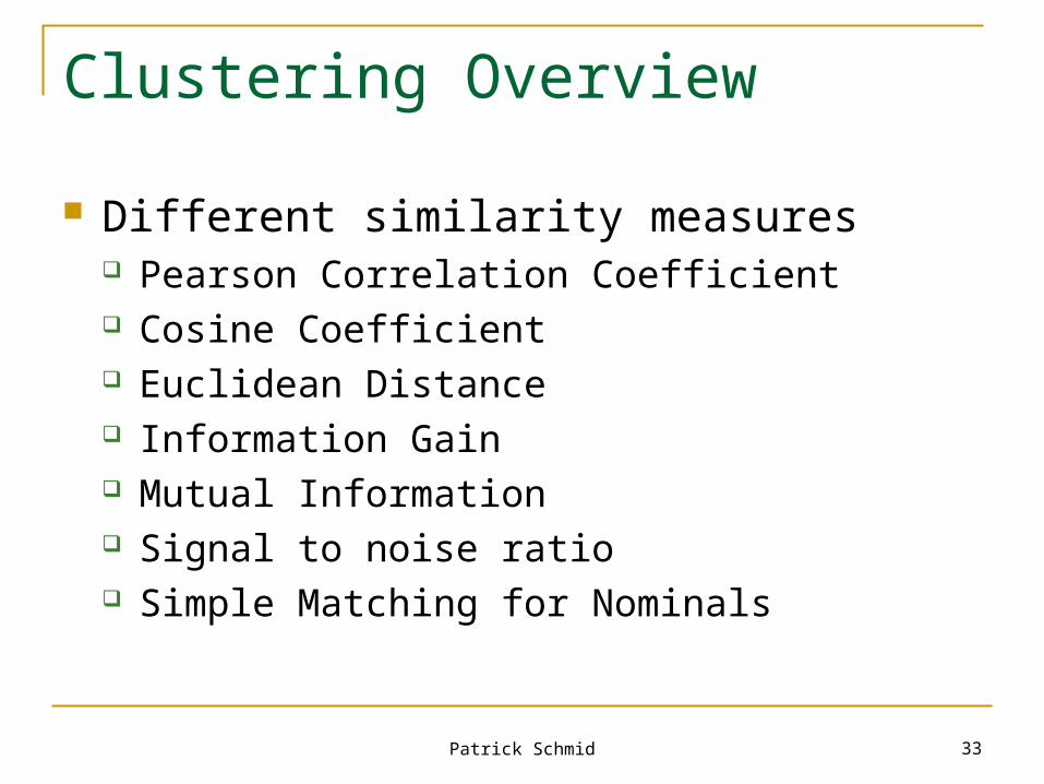
Clustering Overview
Different similarity measures Pearson Correlation Coefficient Cosine Coefficient Euclidean Distance Information Gain Mutual Information Signal to noise ratio Simple Matching for Nominals
Patrick Schmid 34
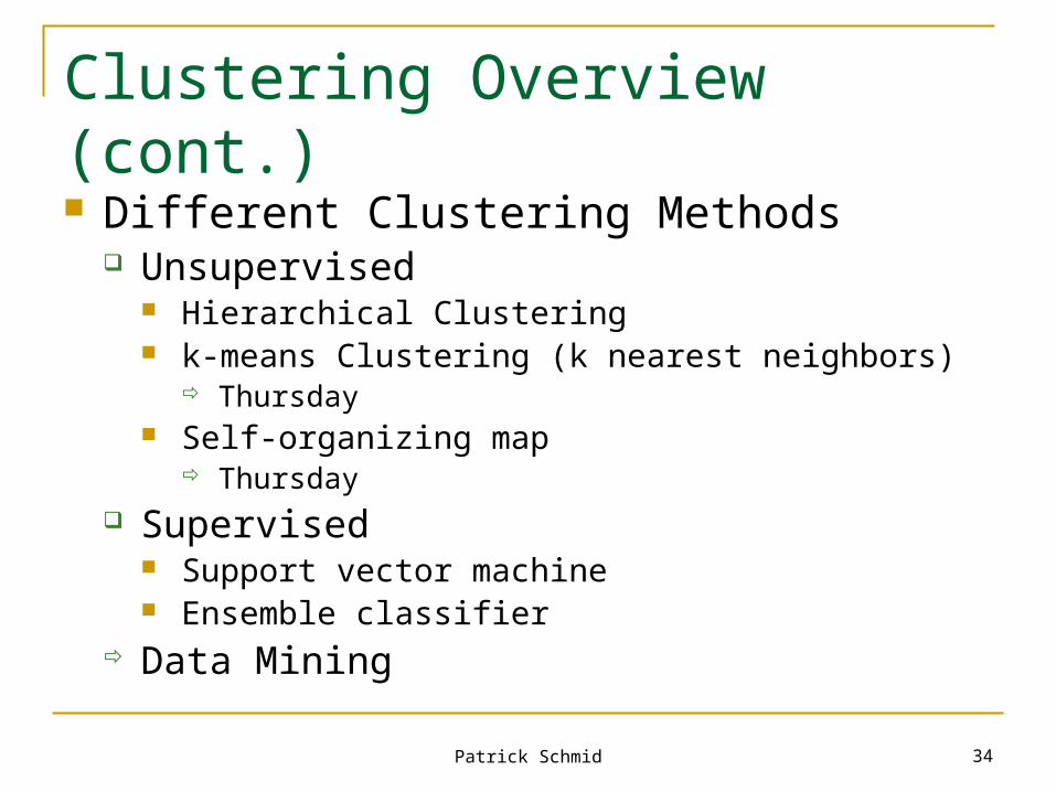
Clustering Overview (cont.)
Different Clustering Methods Unsupervised
Hierarchical Clustering k-means Clustering (k nearest neighbors)
Thursday Self-organizing map
Thursday Supervised
Support vector machine Ensemble classifier
Data Mining
Patrick Schmid 35
Support Vector Machines
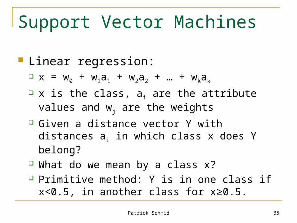
Linear regression: x = w0 + w1a1 + w2a2 + … + wkak
x is the class, ai are the attribute values and wj are the weights
Given a distance vector Y with distances ai in which class x does Y belong?
What do we mean by a class x? Primitive method: Y is in one class if x<0.5, in
another class for x≥0.5.
Patrick Schmid 36
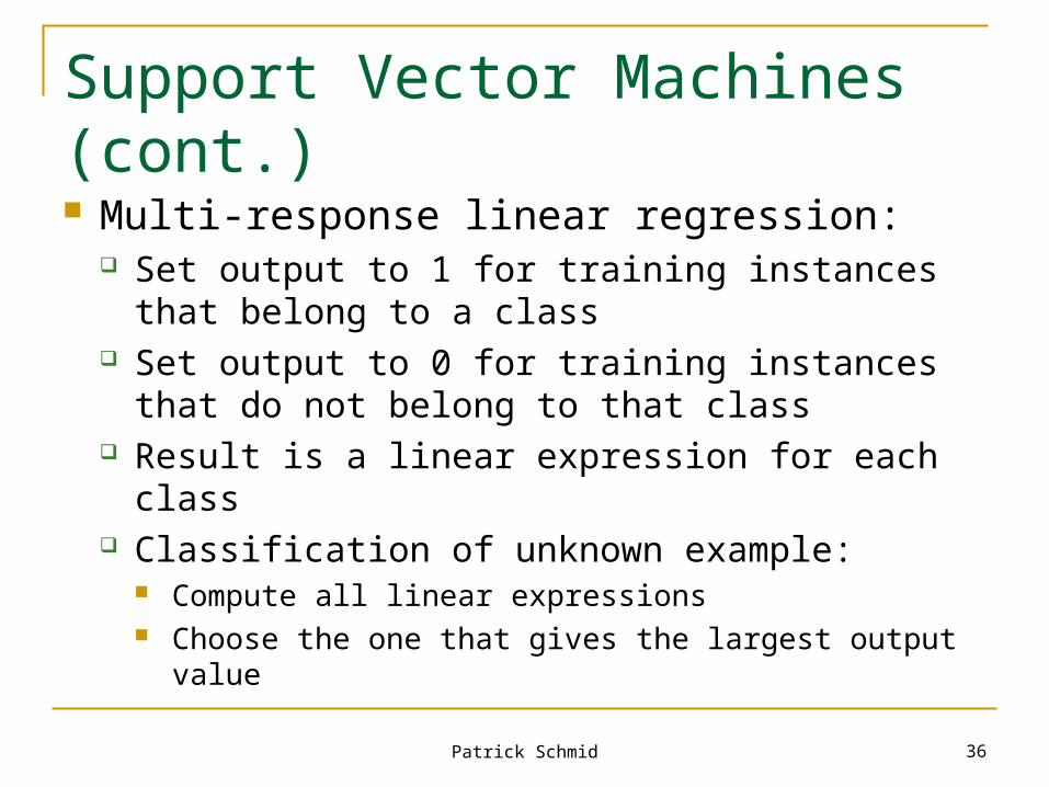
Support Vector Machines (cont.) Multi-response linear regression:
Set output to 1 for training instances that belong to a class
Set output to 0 for training instances that do not belong to that class
Result is a linear expression for each class Classification of unknown example:
Compute all linear expressions Choose the one that gives the largest output value
Patrick Schmid 37
Support Vector Machines (cont.) This means… Two pairs of classes Weight vector for class 1:
w0(1) + w1
(1)a1 + w2(1)a2 + … + wk
(1)ak
Weight vector for class 2: w0
(2) + w1(2)a1 + w2
(2)a2 + … + wk(2)ak
An instance will be assigned to class 1 rather than class 2 if w0
(1) + w1(1)a1 + w2
(1)a2 + … + wk(1)ak > w0
(2) + w1(2)a1 + w2
(2)a2 + … + wk(2)ak
We can rewrite this as (w0
(1) - w0(2)) + (w1
(1) - w1(2)) a1 + … + (wk
(1) - wk(2)) ak > 0
Hyperplane
Patrick Schmid 38
Support Vector Machines (cont.) We can only represent linear boundaries between classes so far Trick: Transform the input using a nonlinear mapping, then construct
a linear model in the new space Example: Use all products of n factors (2 attributes, n=3):
x = w1a13 + w2a1
2a2 + w3a1a22 + w4a2
3
Then use multi-response linear regression However, for 10 attributes and including all products with 5 factors,
we would need to determine more than 2000 coefficients Linear regression is O(n3) in time Problem: Training is infeasible Another problem: Overfit. The resulting model will be “too
nonlinear”, because there are just too many parameters in the model.
Patrick Schmid 39
Support Vector Machines (cont.)
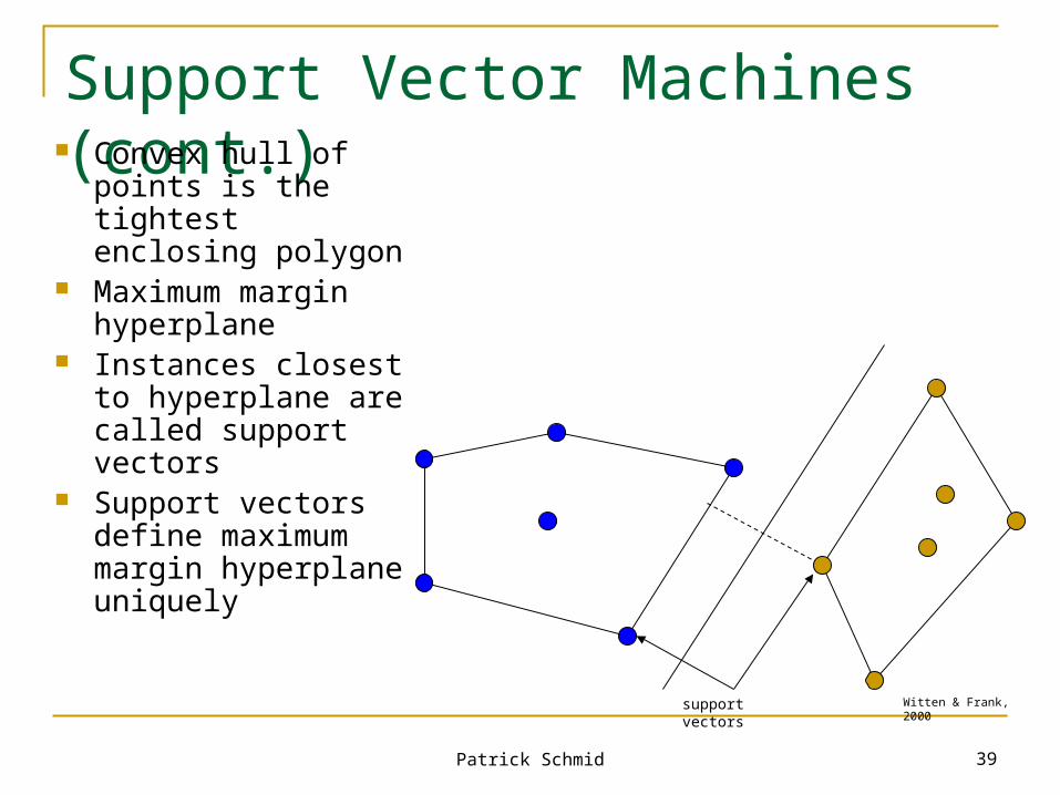
support vectors
Convex hull of points is the tightest enclosing polygon
Maximum margin hyperplane
Instances closest to hyperplane are called support vectors
Support vectors define maximum margin hyperplane uniquely
Witten & Frank, 2000
Patrick Schmid 40
Support Vector Machines (cont.) We only need set of support vectors, everything else is irrelevant A hyperplane separating two classes can then be written as
x = w0 + w1a1 + w2a2 Or
x = b + ∑ αiγi (a(i) ∙ a) i is support vector γi is the class value of a(i) b and αi are numeric values to be determined Vector a represents a test instance a(i) are the support vectors
Determining b and αi is a constrained quadratic optimization problem that can be solved with off-the-shelf software packages
Support Vector Machines do not overfit, because there are usually only a few support vectors
Patrick Schmid 41
Support Vector Machines (cont.) Did I not introduce Support Vector Machines by
talking about non-linear class boundaries? x = b + ∑ αiγi (a(i) ∙ a)n
n is the number of factors (x ∙ y)n is called a polynomial kernel A good way of choosing n is by starting with n=1
and incrementing it until estimated error ceases to improve
If you want to know more: SVMs in general: Witten & Frank, 2000 (lecture material
based on this) Application to cancer classification: Cho & Won, 2003
Demo – Shneiderman
Patrick Schmid 43
References
Brown, P., Botstein, D. “Exploring the new world of the genome with DNA microarrays” Nature genetics supplement, vol. 21, January 1999
Campbell A. & Heyer L. “discovering Genomics, Proteomics, & Bioninformatics” Benjamin Cummings, 2003.
Cheung, V., Morley, M., Aguilar, F., Massimi, A., Kucherlapati, R. & Childs, G. “Making and reading microarrays” Nature genetics supplement, vol. 21, January 1999
Cho, S. & Won, H. “Machine Learning in DNA Microarray Analysis for Cancer Classification” Proceedings of the First Asia-Pacific bioinformatics conference on Bioinformatics 2003 - Volume 19, Australian Computer Society Inc.
Eisen, M., Spellman, P., Brown, P. & Botstein, D. “Cluster analysis and display of genome-wide expression patterns” Proc. Natl. Acad. Sci. USA. Vol 95, pp. 14 863-14868, December 1998. Genetics
Seo, J. & Sheiderman, B. “Interactively Exploring Hierarchical Clustering Results” IEEE Computer, July 2002
Witten, I. & Frank, E. “Data Mining” Morgan Kaufmann Publishers, 2000


