RECOMMENDED PRACTICE DNV GL AS The electronic pdf version of this document found through http://www.dnvgl.com is the officially binding version. The documents are available free of charge in PDF format. DNVGL-RP-O501 Edition August 2015 Managing sand production and erosion
Transcript
RECOMMENDED PRACTICE
DNVGL-RP-O501 Edition August 2015
Managing sand production and erosion
DNV GL AS
The electronic pdf version of this document found through http://www.dnvgl.com is the officially binding version. The documents are available free of charge in PDF format.
FOREWORD
DNV GL recommended practices contain sound engineering practice and guidance.
This service document has been prepared based on available knowledge, technology and/or information at the time of issuance of this document. The use of thisdocument by others than DNV GL is at the user's sole risk. DNV GL does not accept any liability or responsibility for loss or damages resulting from any use ofthis document.
C
hang
es –
cur
rent
CHANGES – CURRENT
GeneralThis document supersedes DNV-RP-O501, November 2007.
Text affected by the main changes in this edition is highlighted in red colour. However, if the changes
On 12 September 2013, DNV and GL merged to form DNV GL Group. On 25 November 2013 Det NorskeVeritas AS became the 100% shareholder of Germanischer Lloyd SE, the parent company of the GL Group,and on 27 November 2013 Det Norske Veritas AS, company registration number 945 748 931, changed itsname to DNV GL AS. For further information, see www.dnvgl.com. Any reference in this document to “DetNorske Veritas AS”, “Det Norske Veritas”, “DNV”, “GL”, “Germanischer Lloyd SE”, “GL Group” or any otherlegal entity name or trading name presently owned by the DNV GL Group shall therefore also be considereda reference to “DNV GL AS”.
On 12 September 2013, DNV and GL merged to form DNV GL Group. On 25 November 2013 Det NorskeVeritas AS became the 100% shareholder of Germanischer Lloyd SE, the parent company of the GL Group,and on 27 November 2013 Det Norske Veritas AS, company registration number 945 748 931, changed itsname to DNV GL AS. For further information, see www.dnvgl.com. Any reference in this document to “DetNorske Veritas AS”, “Det Norske Veritas”, “DNV”, “GL”, “Germanischer Lloyd SE”, “GL Group” or any otherlegal entity name or trading name presently owned by the DNV GL Group shall therefore also be considereda reference to “DNV GL AS”.
involve a whole chapter, section or sub-section, normally only the title will be in red colour.
Main changes August 2015The current 2015 revision includes the following main updates:
a) Document title has been changed from Erosive Wear in Piping Systems to Managing sand production and erosion.
b) Outline and list of considerations for a sand management strategy.c) New guidance on erosion model for flexible pipes with interlock carcass.d) New erosion models for choke valves.e) Guidance on computational fluid dynamics (CFD) erosion modelling.f) Erosion model validation cases.
In addition to the above stated main changes, editorial corrections may have been made.
Editorial corrections
AcknowledgementThe current document is developed in co-operation with a large number of major oil and gas operators. DNV GL is grateful for the financial support to research and development and for being allowed to apply results from projects with these operators to establish this industry guideline.
Recommended practice DNVGL-RP-O501 – Edition August 2015 Page 3
DNV GL AS
C
onte
nts
CONTENTS
CHANGES – CURRENT .................................................................................................. 3
Sec.1 General ......................................................................................................... 61.1 Introduction ...........................................................................................61.2 Application of this document ..................................................................61.3 Reference to codes and standards..........................................................61.4 Abbreviations .........................................................................................71.5 Definitions..............................................................................................71.6 Verbal forms...........................................................................................71.7 Bibliographic references.........................................................................8
Sec.2 Sand management strategy .......................................................................... 92.1 General...................................................................................................92.2 Consequences of sand production ..........................................................92.3 Sand production potential ....................................................................102.4 Philosophy for accepting and managing sand production ....................102.5 Goals and success factors.....................................................................112.6 Premises and acceptance criteria .........................................................11
2.7 Risk assessment...................................................................................132.7.1 Class of erosive service.................................................................132.7.2 Risk assessment and ranking.........................................................14
2.8 Safeguards ..........................................................................................152.9 Strategy implementation......................................................................162.10 Training requirements..........................................................................162.11 Status reporting and periodic revision .................................................16
2.11.1 Status reporting ..........................................................................162.11.2 Revision of strategy .....................................................................16
Sec.3 Fundamentals of particle erosion ................................................................ 183.1 General.................................................................................................18
3.1.1 List of symbols ............................................................................183.1.2 Indexes ......................................................................................193.1.3 Erosive agents.............................................................................203.1.4 Non-erosive agents ......................................................................20
3.2 Characterisation of erosive wear..........................................................213.2.1 Erosion response model ................................................................21
Sec.4 Empirical models for sand particle erosion.................................................. 244.1 General.................................................................................................244.2 Application and limitations...................................................................244.3 Geometry correction factors.................................................................254.4 Model input parameters .......................................................................26
4.4.1 Erosion response model ................................................................264.4.2 Bulk properties ............................................................................264.4.3 Sand content...............................................................................28
Recommended practice DNVGL-RP-O501 – Edition August 2015 Page 4
DNV GL AS
C
onte
nts
4.5 Smooth and straight pipes ...................................................................28
4.6 Welded joint.........................................................................................294.7 Pipe bends............................................................................................304.8 Blinded tee ...........................................................................................314.9 Reducers ..............................................................................................334.10 Intrusive erosion probes .....................................................................344.11 Flexible pipes with interlock carcass ....................................................354.12 Production chokes................................................................................36
4.12.1 General ......................................................................................364.12.2 Choke selection ...........................................................................374.12.3 Operation ...................................................................................384.12.4 Inspection and condition monitoring ...............................................384.12.5 Erosion model for choke gallery .....................................................40
Sec.5 Model parameters for other erosive agents ................................................. 41Sec.6 Software model ........................................................................................... 42App. A Safeguards - managing sand production and erosion.................................. 43App. B Material erosion testing .............................................................................. 48App. C Computational fluid dynamics – erosion simulation .................................... 51App. D Production chokes....................................................................................... 55App. E Model validation.......................................................................................... 59
Recommended practice DNVGL-RP-O501 – Edition August 2015 Page 5
DNV GL AS
SECTION 1 GENERAL
1.1 IntroductionThis recommended practice is developed for the oil and gas industry to provide guidance on how to safely and cost effectively manage the consequences of sand produced from the oil and gas reservoirs through production wells, flowlines and processing facilities. The ultimate goal of this document is to assist prevention of incidents related to sand that may cause harm to people, environment or assets and without causing unnecessary restrictions to production performance.
This document was first developed and issued by DNV in 1996 and has since then only been subject to minor adjustments. The current revision includes more of the background material for the erosion response models and further guidance on development, implementation and follow up of a high-level sand management strategy.
Objective of this document is to provide guidance on how to safely and cost effectively manage the consequences of sand production and erosion through the different stages of design and operation of oil and gas production facilities.
1.2 Application of this documentSec.2 of this document provides guidance on development, implementation and follow up of a field sand management strategy. This section is primarily intended for operating companies, but should also serve as a reference document for engineering companies in different stages of design, fabrication and construction.
Sec.3 to [4.12] of this document provides empirical models for prediction of particle erosion in standard pipework components. The models offer a more specific method for dimensioning of pipework and components exposed to erosive wear compared to the “erosional velocity” approach specified in API-RP-14E or NORSOK P-100. The erosion models may be used to demonstrate compliance between system design, tolerable erosion and sand load either specified in design basis or experienced in operation.
Supporting material relevant for the understanding and transparency of this recommended practice is included in appendices.
1.3 Reference to codes and standards
Document code Title
API-6A Specification for wellhead and christmas tree equipment
API-RP-14E Recommended practice for design and installation of offshore production platform piping systems
API 17J Specification for unbonded flexible pipe
API 17B Recommended practice for flexible pipe
ISO 13703:2000 Petroleum and natural gas industries - Design and installation of piping systems on offshore production platforms
NORSOK P-100 Process systems
NACE Standard MR 0175-93 Sulphide Stress Cracking Resistant Materials for Oil field Equipment
DNV-OS-F101 Submarine Pipeline Systems
Recommended practice DNVGL-RP-O501 – Edition August 2015 Page 6
DNV GL AS
1.4 Abbreviations
1.5 Definitions
1.6 Verbal forms
Abbreviation Description
ALARP as low as reasonable possible
ASR acceptable sand rate
CRA corrosion resistant alloy
DNV Det Norske Veritas
DNV GL Det Norske Veritas Germanischer Lloyds
EOR (IOR) enhanced oil recovery
ESP electrical submerged pump
GLR gas liquid ratio
GOR gas oil ratio
GRP glass fibre reinforced plastic
HDPE high density polyethylene
IOR (EOR) increased oil recovery
MBR minimum bending radius
PCS pipe class specification
PSD particle size distribution
SI special item
WC water cut
Term Definition
C-steel steels containing less than 1.65% manganese, 0.69% silicon and 0.60% copper
corrosion loss of material or loss of material integrity due to chemical or electro-chemical reaction with surrounding environment
droplet erosion loss of material or loss of material integrity due to droplet impact on the material surface
erosion loss of material or loss of material integrity due to solid particle impact on the material surface
erosion-corrosion synergetic effect of erosion and corrosion
low alloyed steel steel containing magnesia, silicon and copper in quantities greater than those for C-steel and/or other alloying elements The total content of alloying elements shall not exceed 5%.
material degradation loss of material or loss of material integrity due to chemical or electrochemical reaction with surrounding environment, or erosive wear resulting from particle and droplet impingement
mixture velocity equal to the sum of the superficial velocities for all phases
oil & gas content in pipe may be either oil or gaspiping system includes pipes for transportation of fluids and associated pipe bends, joints, valves and chokes
The general term covers tubing, flow lines for transportation of processed and un-processed hydrocarbons.
stainless steel steels alloyed with more than 12% Cr (weight)
steel carcass inner steel interlock layer used in flexible pipes for transportation of hydrocarbon fluids
superficial velocity fluid velocities of one phase in piping as if no other fluid phase were present the pipe
Term Definitionshall verbal form used to indicate requirements strictly to be followed in order to conform to this document
should verbal form used to indicate that among several possibilities one is recommended as particularly suitable, without mentioning or excluding others, or that a certain course of action is preferred but not necessarily required
may verbal form used to indicate course of action permissible within the limits of the document
Recommended practice DNVGL-RP-O501 – Edition August 2015 Page 7
DNV GL AS
1.7 Bibliographic references
/1/ deWaard C and Milliams DE. Carbonic Acid Corrosion of Steel, Corrosion, Vol. 31, No 5, 1975.
/2/ deWaard C, Lotz U and Milliams DE. Predictive Model for CO2 Corrosion Engineering in Wet Natural Pipelines, Corrosion, Vol 47, no 12, 1991.
/3/ deWaard C and Lotz U. Prediction of CO2 Corrosion of Carbon Steel, NACE Corrosion 93, Paper no 69, 1993.
/4/ Ikeda A, Ueda M, Vera J, Viloria A, Moralez JL. Effects of Flow Velocity of 13Cr, Super 13Cr and – Duplex Stainless Steels.
/5/ Raask E. Tube erosion by ash impaction, Wear No. 13, 1969
/6/ Tilly GP. Erosion caused by Impact of Solid Particles, Treatise of Material Science and Technology, Volume 13, 1979.
/7/ Finnie I. Erosion of Surfaces by Solid Particles, Wear 1960.
/8/ Haugen K, Kvernvold O, Ronold A and Sandberg R. Sand Erosion of Wear Resistant Materials, 8th International Conference on Erosion by Liquid and Solid Impact, Cambridge 1994.
/9/ Lindheim T. Erosion Performance of Glass Fibre Reinforced Plastics (GRP).
/10/ Hansen JS. Relative Erosion Resistance of Several Materials, ASTM STP 664, 1979.
/11/ Kvernvold O and Sandberg R. Production Rate Limits in Two-phase Flow Systems – Sand Erosion in Piping Systems, DNV Report No. 93-3252, 1993.
/12/ Huser A. Sand erosion in Tee bends. Development of correlation formula DNV Report No. 96-3226, 1996.
/13/ Oka YI, Okamara K, Yoshida T. Practical estimation of erosion damage caused by solid particle impact. Part 1: Effects of impact parameters on a predictive equation, Wear 259 (2005) 95-101
/14/ Oka YI, Yoshida T. Practical estimation of erosion damage caused by solid particle impact. Part 2: Mechanical properties of materials directly associated with erosion damage, Wear 259 (2005) 102-109
/15/ Barton NA. TÜV-NEL-Research report 115. Erosion in elbows in hydrocarbon production systems: Review document, 2003
/16/ IJzermans S, Helgaker JF. Large Scale Erosion Testing of a Flexible Flowline. AOG Conference, 12th of March 2015
/17/ Kvernvold O, Torbergsen LE, Eriksen R (DNV) and Kjørholt H (Statoil). New Strategy for Sand Management to safely Improve Production Performance Deep Offshore Technology Conference; USA November 2002
/18/ Selfridge F, Munday M (DNV), Kvernvold O (DNV), Gordon B (ConocoPhillips). Safely Improving Production Performance through Improved Sand Management, SPE-83979, 2003
/19/ Emiliani CN, Lejon K (Statoil), Lindén M, Engene J, Kvernvold O (DNV), Packman C (Roxar), Clarke D (Cormon), Haugsdal T (Clampon). Improved Sand Management Strategy: Testing of Sand Monitors under Controlled Conditions, SPE-146679, 2011
/20/ Lejon K, Reme AB, Woster RB, Kvernvold O, Torbergsen L. Sand Production Management for Snorre B Subsea Development – Lessons learned and actions taken, DOT, 2007
Recommended practice DNVGL-RP-O501 – Edition August 2015 Page 8
DNV GL AS
SECTION 2 SAND MANAGEMENT STRATEGY
2.1 GeneralThe purpose of this chapter is to describe an industry practice applicable to subsea, topside and onshore oil & gas production facilities. In addition to the general guidance provided in this document the basis for a sand management strategy needs also to consider local regulations, company specific requirements and guidelines, field specific system layout and operational experience.
The current chapter provides guidance on how to establish, document and follow up a strategy for managing sand production, considering the following key topics:
— sand production potential— consequences of sand production— philosophy for accepting and managing sand production — goals and success factors— premises and acceptance criteria — risk assessment— safeguards — strategy implementation— training requirements— production optimisation — condition monitoring and inspection— status reporting and revision of strategy.
As a first principle the sand management strategy shall address all systems that are considered likely to be exposed to solids produced from well. The upstream and downstream battery limits for the strategy shall therefore be properly defined. Both passive and active means to control and monitor sand production and the associated consequences should be considered.
2.2 Consequences of sand productionSand production can have significant consequences for both the production and the assets. Key failure modes are related to erosion, sand accumulation, plugging or contamination by sand. For the majority of oil & gas fields, sand from the reservoir formation is an inevitable by-product. Monitoring and controlling sand production is important for the following reasons:
— Sand may cause damage to well components such as sand screens, tubing, down-hole safety valves or electrical submersed pumps (ESPs).
— Sand may cause erosion in piping system and components that if undetected may lead to loss of containment.
— Sand may cause erosion in blow-down systems during ESD depressurization or inadvertent routing of production to knock-out drum. Particular focus should be on flow restrictions (valves or orifice) and immediate piping downstream due to potentially high gas velocities resulting from pressure let-down. Low wall thickness characteristic for flare systems should be acknowledged.
— Sand may accumulate in wellbore if wells are produced below lifting rate for sand, ultimately leading to sanding-in and loss of well.
— Accumulation of sand in production lines may affect corrosion rates, cause upsets during pigging operations or increased pressure resistance during operation.
— Accumulation of sand in separators may cause reduced separation efficiency and carry-over of sand to downstream systems that are not designed for or have little tolerance for sand.
— Instrumentation may be influenced, potentially affecting safety critical systems for shut-down or process control.
— Challenges with sand volume handling capacity and removal of sand from the process may cause upsets or unplanned shut-downs.
Recommended practice DNVGL-RP-O501 – Edition August 2015 Page 9
DNV GL AS
— Sand production may influence produced water quality in a negative direction.
— Overboard disposal of produced water containing sand may cause erosion to pipework and components or reduced well injectivity if re-injected.
— Accumulation of sand in process- or safety critical valves may impair valve performance due to blockage or increased friction.
— Sand may damage rotating equipment such as pumps (and compressors).— Particularly for non-corrosion resistant materials, even a moderate sand erosion potential may affect
flow accelerated corrosion (FAC).
2.3 Sand production potentialThe potential for sand particles being released and transported from formation to wellbore is determined by a number of complex factors requiring expert evaluation by reservoir geologists and completion engineers. The sand potential is normally assessed based on knowledge available early in the field concept development; however the information available at this point is often fairly limited and associated with significant uncertainty.
It is not the purpose of this document to provide guidance on how to assess sand production potential, rather to provide a sufficient description of the key parameters relevant for managing sand production in field operation.
Different formations have different mechanical strength. Rock strength is characterised in terms of level of consolidation which describes how well sand grains are “cemented” together. Rock-strength is normally determined based on core-sample testing, and the corresponding sand potential is assessed for the field life considering the planned recovery strategy. It should be acknowledged that core samples normally taken from exploration wells are not necessarily representative for all subsequent production wells and therefore associated with uncertainty. The true sand potential will also be a function of the actual reservoir recovery strategy during field life. A reduction in reservoir pore pressure will increase the load from the overburden on the rock formation, which in turn will increase the potential for “rock failure” and formation of sand grains. This explains why sand production is often experienced to increase in tail end- and low pressure production.
Water increases the mobility of sand to well bore due to reduced surface tension between sand and water compared to sand and oil/gas and potentially increased drag on the sand grains. Onset of sand production is therefore often found to coincide with onset of water production.
Rapid transients in well operation may also affect the near well bore zone in a negative direction causing increase in sand production and should therefore to the extent possible be avoided.
2.4 Philosophy for accepting and managing sand production Adopting a philosophy of “zero” sand production will in many cases put significant restrictions on the field production potential or cause premature abandonment of wells. A sand management strategy should therefore be based on a combination of minimising sand production by means of sand control where it is commercially viable and practicable to do so and managing with the consequences of sand production experienced in operation. Allowing for a certain sand production that can be safely and effectively managed may also significantly increase the field production potential.
Managing sand production means allowing for sand production from individual wells and through co-mingled streams depending on consequences for integrity and/or availability of the facilities. This enables optimisation of production from different wells and sub-systems, hence preventing unnecessary restrictions without compromising on safety and reliability of the system.
For a given combination of field design and operating conditions the acceptable sand rate (ASR) will be limited by the following two main factors:
— acceptable rate of consumption of erosion allowance for production piping and components— sand volume handling capacity in the process, cleaning and disposal system.
A prerequisite for this philosophy is that a sufficient system for continuous monitoring of operating
Recommended practice DNVGL-RP-O501 – Edition August 2015 Page 10
DNV GL AS
conditions and sand production combined with facilities for handling of sand in the process system is in
place. Adopting an ASR philosophy should be subject to a risk assessment where the required safeguards for managing the consequences are established and followed up, ref [2.7].
The strategy for how to manage sand should be outlined early in the field development to ensure appropriate sizing and selection of equipment and instrumentation for monitoring, controlling and handling of sand production. The strategy should reflect both methods to control and monitor sand production and appropriate safeguards to control the risk. The strategy should also be aligned with the overall Asset Integrity Management System for the production facilities.
2.5 Goals and success factorsThe overall goals for a sand management strategy should be defined and validated on regular intervals, aiming for:
— no loss of product to environment due to failures caused by erosion— no erosion damages causing unplanned shut-down or maintenance/repair/replacements— limited (acceptable) process upsets due to sand production, accumulation, cleaning and disposal— quality of disposed produced water/sand in compliance with operator and authority requirements— maximized production potential (no unnecessary restrictions due to sand).
The following key factors should be considered for a successful implementation and adherence to the strategy:
— High level of knowledge within the field organisations related to the consequences of sand production.— Clearly defined roles and responsibilities related to follow up of safeguards.— Comprehensible steering criteria related to allowable sand production for the individual wells and
systems.— Systems in place for monitoring and reporting the effects of combined operating conditions and sand
production.— Confirmed correspondence between systems for monitoring the effects of sand production (erosion and
deposition) and results from inspection and maintenance campaigns – building confidence in the strategy.
2.6 Premises and acceptance criteriaThe strategy shall be based on the specific system design, field development strategy and operation. The premises for the strategy should be established prior to performing the risk assessment (ref. [2.7]) and should as a minimum consider the following:
— reservoir conditions and planned recovery strategy— formation strength, expected sand potential and sand control— sand characterisation, particle size distribution (PSD) and fraction of erosive agents— general field layout: considering subsurface, subsea and topside or onshore facilities - limited upstream
by the lower completion of the production wells and downstream by the battery limits where the processed stream can be considered free from solids
— specifications for piping system, manifolds, flowlines and components with respect to geometrical layout, sizing and tolerable erosion
— process conditions— sand handling capacity in the process system, considering methods for sand removal, cleaning and
disposal— safe envelope for sand transport, considering production wells, flowlines and pipework— field service life, also considering potential plans for life time extension (IOR/EOR)— implemented safeguards related to design, procedures and instrumentation for follow up of sand
production and its consequences— operational experience
Recommended practice DNVGL-RP-O501 – Edition August 2015 Page 11
DNV GL AS
— planned future modifications, considering new tie-ins or change in process conditions
— field organisation and responsibilities— company specific requirements— local regulations.
2.6.1 Tolerable erosionAn absolute “zero” tolerance for erosion is difficult to relate to from a practical perspective, hence a minimum tolerance for erosion needs to be specified. An acceptable erosion rate (e.g. mm/yr) needs to consider the remaining target service life of the system and the complexity and cost of system repair or replacement.
For steel pipework tolerable erosion should be identified with reference to one of the following options:
— Allow for a minimum erosion allowance of 0.5 mm (1/50”) with reference to typical accuracy of hand-held UT equipment for wall thickness measurements.
— Erosion allowance according to pipe class specification (PCS).— Acceptable utilisation of corrosion allowance or CRA cladding noted in PCS. To what extent the corrosion
allowance can be utilised as erosion allowance needs to consider the level of corrosive service. For components with internal CRA cladding, the erosion allowance may be taken as a percentage of the cladding thickness.
— Erosion allowance identified based on minimum wall thickness requirement according to specified system pressure rating (pipe stress analysis may be required for this option).
— De-rating of the system to increase tolerable erosion should only be considered as a last option, and should be subject to a thorough assessment also considering future operation of the system.
For special items the erosion allowance should be advised by vendor, considering potential effects on functionality, performance or containment. E.g. for flow meters erosion may affect meter calibration, for choke valves erosion may affect controllability and for cyclone units erosion may affect separation performance.
2.6.2 Sand handling capacityTo minimise process upsets and to reduce erosion potential, sand should be separated from the process stream as early in the process as possible. In most cases this will be the inlet separator(s) for the process train. The standard approach is to let the sand separate with the liquid phase by gravity and accumulate in the bottom part of the separator, ref. Figure 2-1. Acceptable sand accumulation (before removal is required) depends on a number of complex factors such as separation efficiency, method of removal and sand carry-over to downstream process systems. In many cases carry-over of smaller particles to downstream systems cannot be fully avoided and needs to be managed, and the consequences need to be assessed.
General requirements to systems for removal of sand from process vessels are given in /NORSOK P100; section 5.2.4.4/.
For process vessels where sand needs to be removed manually, the sand handling capacity should be limited to an acceptable sand build up between planned intervals for manual removal. Manual removal will in most cases require process shut-down having significant impact on plant availability. From operational experience the total sand volume accumulation that can be accepted is typically in the order of 1-3 m3 depending on vessel size, configuration and operation. Given a typical interval of 3 years between major maintenance (emptying of the separator) this means that a maximum sand production of approximately 1 m3/year can be tolerated. This is equivalent to around 2 tons of water saturated sand.
For process vessels with fully or partially automated systems for sand removal, the sand volume handling capacity may be determined from the acceptable volume of sand build-up and frequency of sand removal. Intervals between sand removals typically range from a few days to several weeks, depending on actual sand production. During the sand removal sequence (flushing) the quality of produced water may be affected in a negative way. In service, the interval between sand removals should be optimised based on experience and may vary over the field life. A partially or fully automated system for sand removal significantly increases the sand volume handling capacity. From operational experience sand loads in the order of 100 m3/yr has safely been handled for a single platform (separator).
Recommended practice DNVGL-RP-O501 – Edition August 2015 Page 12
DNV GL AS
Where practically and economically viable to do so, installation of wellhead or in-line de-sanders may
significantly reduce sand loading for inlet separators, thus reducing negative consequences associated with sand removal and process upsets.
Figure 2-1 Typical sand deposition in horizontal process vessel with conventional sand removal system
2.7 Risk assessmentAs basis for the sand management strategy a risk assessment should be performed to identify both threats and opportunities associated with sandy service operation. The purpose of the risk assessment is to ensure that sufficient, effective and manageable safeguards are in place in order to be prepared for, detect and handle sand production.
In the early concept and design phase the risk assessment may be limited to a high level assessment considering sand and erosion potential and the requirements to sand handling capacity. The importance of an early outline of a sand management strategy relates to decision of:
— need for sand control— sizing of flowlines, pipework and components — instrumentation for monitoring sand production and erosion — systems for removal, cleaning and disposal of sand from process systems.
For the operations phase the risk assessment should be performed by a dedicated sand management team involving representatives from relevant disciplines in the operating organisation. It should be emphasized that a successful implementation of a sand management strategy requires a cross-discipline approach.
2.7.1 Class of erosive serviceRanking of the erosion potential for pipework may be performed with reference to calculated bulk flow velocities, considering that the flow velocity determines the order of magnitude for erosion. The class of erosive service for pipework provides a simple indication of whether a system is susceptible to erosion. In reality, the exact size and geometrical shape of the pipework components in combination with sand particle size and fluid properties such as density and viscosity will influence the actual erosion potential per amount of sand.
Bulk flow velocities may be available in the production control system or be calculated based on a simplified black oil model ([4.4.2]) with reference to allocated or measured flow rates, operating pressures and temperatures.
The erosion classes defined in Table 2-1 may be applied to identify whether a given operating condition for a given pipework system may be susceptible to erosion. The relative erosion potential referring to erosion class (1) demonstrates the order of magnitude increase in erosion potential as function of increase in bulk flow velocity.
Recommended practice DNVGL-RP-O501 – Edition August 2015 Page 13
DNV GL AS
When increasing the bulk flow velocity from erosion class (1) to erosion class (3) the expected erosion for
a given sand load (kg) increases by a factor of 100. Similarly if the velocity is increased to erosion class (6) the erosion potential increases by a factor of approximately 5000. In other words the amount of sand required to cause similar erosion damage in a pipework system operated in erosion class (1) is in the order of 5000 times higher than for a system operated in erosion class (6).
2.7.2 Risk assessment and rankingThe risk assessment and -ranking should be performed based on a breakdown of the system into sub-systems that is considered practical with reference to operator’s organisation and responsibilities of different disciplines. A typical system breakdown is suggested below as a starting point:
— lower well completion, considering sand screens, tubing or other inflow control components — down hole safety valve— down hole artificial lift systems (gas lift, ESP)— XT and valves — pipework and components between XT and manifold— production choke— instrumentation and metering systems— manifolds— flowlines and risers— boosting systems for unprocessed flow— pipework between manifold and first process vessel— process vessels (separators) and internals— produced water system from separators, pipework and components— produced oil system from process vessels, pipework and components — blow down systems and equalisation manifolds— water injection systems, components
Table 2-1 Class of erosive service
ErosionClass
Pipework Bulk Flow Velocity
Vm (m/s)Definition
Relative erosion
potential 1)Description
6 50 - 70 Extremely high erosion potential 5000
System needs to be operated close to sand free. Safeguards to monitor erosion should be in place and closely monitored
5 30 – 50 Very high erosion potential 1500 Tolerable sand production limited by risk of
erosion
4 20 – 30 High erosion potential 500Tolerable sand production will in most cases be dictated by erosion rather than sand handling capacity
3 10 – 20 Medium erosion potential 100 Tolerable sand production may be limited both by erosion and sand handling capacity
2 5 – 10 Low erosion potential 25
A large amount of sand is required to cause erosion. The acceptable sand load will in most cases be limited by the sand handling capacity in the process system
1 0 – 5 Extremely low erosion potential 1
Effects of plain erosion, i.e. not considering any combined effects of flow accelerated corrosion, can normally be neglected for realistic sand loads
1) Relative erosion potential is given for the average velocity in each velocity interval
Recommended practice DNVGL-RP-O501 – Edition August 2015 Page 14
DNV GL AS
— safety critical instrumentation.
For each of the sub-systems, the risk associated with sand production should be assessed on a qualitative basis with reference to the risk categories suggested in the table below.
The risk assessment should address:
— critical system functions— consequence of each failure mode related to sand— acceptance criteria related to containment, function, availability and performance— safeguards – risk reducing measures— risk level with and without active safeguards.
The risk associated with sand production should be made visible both with and without safeguards to emphasize the importance of following up both active and passive safeguards.
2.8 Safeguards Possible safeguards to control sand production and manage its consequences within acceptable limits are listed below and further elaborated in App.A:
— mechanical sand control — draw-down control — optimisation of artificial lift mechanism — periodic testing of safety critical valves— continuous monitoring and control of sand production— spot-check sampling of sand production (e.g. routing of well to test separator, sand traps)— erosion modelling— continuous monitoring of erosion (e.g. erosion probes)— monitoring by calculations; control of flow velocities— monitoring choke condition and operation— monitoring sand-build-up in process vessels— wellhead or in-line de-sanders— removal of sand from process vessels— monitoring of flow velocities in processed liquid streams— pigging (mechanical or hydraulic) of infield flowlines— online NDT— inspection.
It should be acknowledged that some of the safeguards are inherent to system design (passive) and that others require continuous follow up (active). The relevance, feasibility and effectiveness of the individual safeguard needs to be evaluated on a case to case basis as part of the risk assessment.
Table 2-2 Risk ranking
Risk Definition
HighRisk associated with sand production in conflict with acceptance criteria or non-compliance with standards or regulations. System cannot be operated without modifications to system or operating procedures, or with additional safeguards
Medium Risk acceptable. Additional monitoring or safeguards shall be evaluated by operator according to ALARP principle.
Low Low risk with current operational procedures and safeguards
Recommended practice DNVGL-RP-O501 – Edition August 2015 Page 15
DNV GL AS
2.9 Strategy implementation
The sand management strategy should include a sand management manual that provides a description of activities and responsibilities related to follow up of critical safeguards identified in the risk assessment. Definition of the person/group responsible for each activity should be as simple and specific as possible to avoid diffusion of responsibility.
The sand management manual should serve as a practical guideline in daily operation. Sufficient guidance should be included to ensure that activities are correctly and effectively executed, reported and communicated. Where practicable to do so, reference shall be made to relevant operating procedures.
2.10 Training requirementsRequirements to personnel training should be decided with reference to the activities and responsibilities dedicated to specific personnel as described in the sand management manual. A general description of the specific field sand potential and strategy for managing sand production should be included as part of this training.
2.11 Status reporting and periodic revision
2.11.1 Status reportingA periodic sand management status report should be established typically on a 12 month cycle. The overall objective of the status report is to identify, communicate and execute necessary actions to adjust the strategy or its application:
— confirm that the objective of the sand management strategy is met for the reporting period— provide input to inspection planning — ensure that modification to the production system or operating conditions relevant for the next period
are identified and implemented in the sand management strategy. — provide basis for production optimisation considering any limitations imposed by sand production— capture any incidents/failures related to sand production over the last period of operation.
2.11.2 Revision of strategyThe sand management strategy should be subject to periodic audit/review, e.g. on a 12 month cycle. Related to the previous production period the following questions (check list) should be addressed and relevant actions identified if answered confirmative:
— erosion in piping systems or components has resulted in loss of containment (external leakage)— erosion has resulted in excessive consumption of erosion allowance – identified from inspection— erosion has led to unplanned replacement of components— observed unacceptable process upsets due to (jetting), cleaning or disposal of sand— observed significant and frequent non-compliance with produced water quality— observed non-compliance with acceptable oil in disposed sand— systems for sand monitoring not calibrated according to plan— significant production potential is restricted due to sand production — other identified issues not covered by the above.
Related to the next 12 month period the following questions (check list) should be addressed and relevant actions identified if answered confirmative:
— development of and tie-in of new production facilities— modifications to existing production facilities; piping, valves, instrumentation and chokes will be
implemented for next period— process conditions will be significantly changed for next period (Pressure, WC, GOR, …)— identified down hole sand control failures or significant increase in sand production
Recommended practice DNVGL-RP-O501 – Edition August 2015 Page 16
DNV GL AS
— modification of acceptance criteria, e.g. de-rating of systems increasing erosion allowance or improved
sand handling capacity— modifications to established procedures for sand monitoring.
The sand management strategy should be updated based on the output from the audit/review as found required.
Recommended practice DNVGL-RP-O501 – Edition August 2015 Page 17
DNV GL AS
SECTION 3 FUNDAMENTALS OF PARTICLE EROSION
3.1 GeneralThe selection of materials and dimensioning of pipes are performed in order to obtain necessary strength, capacity and service life to cope with the production conditions. Material degradation due to corrosion, erosion and/or erosion-corrosion, may gradually affect the integrity of the piping system. Material degradation will generally depend on the production characteristics for the system; i.e. production rates, pressure and temperature, and the presence of corrosive components and erosive solid particles. The degradation may also be strongly dependant on the pipe material.
Material degradation can in most cases not be fully avoided, but the material may be allowed to degrade to a certain extent and in a controlled manner. By proper dimensioning, selection of suitable materials, use of inhibitors or other corrosion/erosion reducing measures and/or by application of corrosion/erosion allowance, a system which fulfils the requirements can generally be achieved. Selection of such measures may, however, be associated with high cost.
The current section describes the fundamental theory for plain particle impact erosion, providing the basis for the empirical erosion models in Sec.4 and detailed CFD erosion simulations described in App.C of this document.
3.1.1 List of symbols
Symbol Description Unit
A dimensionless parameter group [-]
At area exposed to erosion [m2]
Apipe cross sectional area of pipe [m2]
Aratio area ratio between cross sectional area in reducer [-]
b function of Re [-]
C1 model/geometry factor [-]
C2 particle size correction factor [-]
Cunit unit conversion factor (m/s ~ mm/year) [-]
c function of Re [-]
D inner pipe diameter [m]
dp particle diameter [m]
dp,c critical particle diameter [m]
E actual surface thickness loss [m]
Em actual material loss rate [kg/s]
Em,m relative material loss rate [kg/kg]
EL actual surface thickness loss rate [m/s]
EL,m relative surface thickness loss [m/kg]
EL,y annual surface thickness loss [mm/year]
EL,measured measured surface thickness loss [mm/year]
F(α) function characterising ductility of material [-]
G corrections function for particle diameter [-]
h height of weld reinforcement [m]
K material erosion constant [(m/s)-n]
k material constant
mass flow of gas in pipe [kg/s]
ml mass flow of liquid in pipe [kg/s]
Mp mass of sand [kg]
mp mass rate of sand [kg/s]
gm
Recommended practice DNVGL-RP-O501 – Edition August 2015 Page 18
DNV GL AS
3.1.2 Indexes
mm total mass rate of fluids [kg/s]
R radius of curvature given as Number of Internal Pipe Diameters. Reference of radius of curvature is centreline of pipe
[-]
Re Reynolds number [-]
Up particle impact velocity (equal to mixture fluid velocity) [m/s]
Vm1, Vm2 fluid velocity in cross section 1 and 2 of reducer [m/s]
Vgs superficial velocity of gas phase in piping [m/s]
Vls superficial velocity of liquid phase in piping [m/s]
Vm mixture fluid velocity in piping [m/s]
α particle impact angle [rad]
β = ρp/ρm density ratio between particle and fluid [-]
γ = dp/D ratio of particle diameter to geometrical diameter [-]
Recommended practice DNVGL-RP-O501 – Edition August 2015 Page 19
DNV GL AS
3.1.3 Erosive agents
Erosion models given in the current document are derived and validated primarily for quartz sand; however the models may also be applied to provide estimates of erosion potential for other erosive agents. The most common erosive agents causing particle erosion in oil and gas systems for which the erosion models given in the current document may be applied are described below. For other erosive agents than quartz sand, guidance is given in Sec.5.
3.1.4 Non-erosive agentsNon-erosive solids are defined as solids having a sufficiently low hardness or size not to cause erosion to a material either as a result of surface ductile deformation or fatigue. Particles with hardness on Mohs scale less than 3 can normally be considered non-erosive to steel, see table below.
SandSand produced from oil & gas formations may vary in terms of size, quartz content, shape and sharpness. All these factors affect how erosive the sand will be to an exposed surface. In terms of size, sand is defined as particles in the range 62 – 2000 µm [W.C. Krumbein & L.L. Sloss]. Particle erosion is governed by the sand quartz fraction. On the Mohs hardness scale quartz has a hardness of 7, making it erosive to a wide range of construction materials. Particles of size less than 62.5 µm are classified as fines. Erosion models described in the current document are limited to particle sizes above 20 µm. Fines are normally less erosive than sand both due to particle size and quartz content. Particle sizes limited to fines can be achieved with various methods for down-hole sand control. Conservatively the erosive character of fines can be assumed as for sand. Particles larger than 2000 µm are classified as gravel.
Barite / CalciteBarite and Calcite used for weighting of drilling, completion and kill fluids. On the Mohs hardness scale these materials have hardness in the order of 3 making it significantly less erosive to steel compared to quartz particles. Characteristic particle size when used as weight material is in the order of 20 µm. Mixed in high density liquid fluids the small particle sizes will also supress erosion. For normal circulation rates the erosion potential is expected to be low, however under certain conditions a combination of high velocities and large amounts of weight material may cause erosion.
ProppantsProppants are customised particle distributions either based on treated sand or made artificially. Proppants are used e.g. for hydraulic fracking operations or for packing of sand screens. In some cases proppants may be produced back to the production facilities and cause similar concerns as sand produced from the formation. For steel, proppants may be equally erosive as quartz sand. From erosion testing variations are observed between intact and crushed proppants.
Sodium Chloride (salt)Sodium Chloride (2.5 on the Mohs scale) used as weight material for brine can be considered non-erosive to steel for bulk flow velocities less than 100 m/s.
Clay/Silt Clay particles (2-2.5 on the Mohs scale) can be considered non-erosive to steel for bulk flow velocities less than 100 m/s
Recommended practice DNVGL-RP-O501 – Edition August 2015 Page 20
DNV GL AS
3.2 Characterisation of erosive wear
3.2.1 Erosion response modelThe terms erosive wear and erosion are in the present document defined as material loss resulting from impact of solids/sand particles on the material surface, ref. Figure 3-1.
Figure 3-1 Notation - particle impact velocity and angle
Erosive wear can be estimated from the following expression /8/, /13/, /14/, provided impact velocities and angles are known for the particles impacting on the target surface, ref. Figure 3-1:
The function F(α) characterises the ductility of the target material. Steel grades are generally regarded as ductile, while cermets like tungsten carbide with a metallic binder phase are defined as brittle.
Coatings may be ductile or brittle depending on chemical composition and deposition method. Metallic or hard coatings are applied by thermal spraying, overlay or galvanic plating methods. Soft coatings are defined as polymeric/epoxy coatings and are ductile in nature.
Ceramics are generally characterised as brittle materials. The particle impact velocity (Up) is linked to the flow velocity either through specific correlations accounting for slip velocity or calculated directly by a particle drag model. The material coefficients (K) and (n) are derived from testing for a given combination of material and erosive agent. Coefficients for selected ductile and brittle materials are given in Table 3-1.
Angle dependency for ductile and brittle materials are given in the expressions below and illustrated graphically in Figure 3-2. Ductile materials experience maximum erosion for impact angles in the range 20 to 50°. Brittle materials experience maximum erosion at 90° (π/2) impact angle and erosion is gradually reduced for smaller angles. The linear F(α) for brittle materials shall be considered an approximation, however sufficient for most practical applications.
Recommended practice DNVGL-RP-O501 – Edition August 2015 Page 21
DNV GL AS
Figure 3-2 Characteristic particle impact angle dependency for erosion of ductile (steel) and brittle materials
Erosion potential for a given particle impact characteristic is directly proportional to the amount of particles exposed to the surface, independent of time. This is valid as long as the particle concentration in the fluid is sufficiently low (< 500 ppmV)1) to avoid any significant particle-particle interaction. 1) For erosion testing the sand concentration should conservatively be kept below 100 ppmV (100 cm3 of sand per 1 m3 of fluid).
Within the typical operating temperature for oil and gas facilities (<200°C), variation in plain particle erosion as function of temperature can normally be neglected.
For velocities lower than 100 m/s, the difference in erosion resistance for relevant steel grades is generally within ±25%. This also applies to Ni-based alloys typically used in piping systems.
Recommended values for the most commonly used materials and an erosive agent equivalent to quartz sand are given in Table 3-1.
The parameters are determined according to test procedure given in App.B. Correction factors for other relevant erosive agents than quartz sand are given in Table 5-2.
Brittle materials:
(3.4)παα ⋅= 2)( brittleF ; [ ]1,0)( ∈αF for
∈
2,0 πα
Recommended practice DNVGL-RP-O501 – Edition August 2015 Page 22
Recommended practice DNVGL-RP-O501 – Edition August 2015 Page 23
DNV GL AS
SECTION 4 EMPIRICAL MODELS FOR SAND PARTICLE EROSION
4.1 GeneralThe following sections provide empirical models for estimation of erosive wear in typical steel piping components. The models and recommendations have been worked out based on experimental investigations available in literature, dedicated erosion tests and experience and models available within DNV GL. The majority of experimental validation data have been obtained at low/moderate pressures in smaller diameter test facilities. Extrapolation to higher pressure conditions and larger diameter pipes has been performed based on detailed CFD erosion simulations and also by comparison with field experience. A selection of controlled validation cases is included in App.E.
4.2 Application and limitationsThe models described in the following sections only address plain erosion, i.e. do not account for potential combined effects of corrosion and particle erosion, flow accelerated corrosion (FAC) or other mechanisms such as droplet erosion or cavitation. Additional wear due to these effects needs to be considered separately.
Application of the erosion models should be limited to quartz sand as the erosive agent, unless otherwise specified. Guidance on how the models may be used for other erosive agents is given in Sec.5 of this document. The erosion models are developed for what is considered realistic particle concentrations, i.e. concentrations sufficiently low to assume marginal particle-particle interaction. Hence, the models may be conservative for particle concentrations above typically 500 ppmV.
All models are based on mixture fluid properties. For single phase fluids (liquid or gas) the single phase properties shall be applied. For multiphase flow the mixture properties shall be established based on the superficial velocities and single phase properties according to recommendations given in the current document. The models are based on the assumption of a minimum straight upstream pipe section corresponding to 10 pipe diameters. For complex pipework, an appropriate geometry correction factor according to [4.3] shall be applied. Application of the models should be limited to the range specified for input parameters in Table 4-1.
Table 4-1 Limitations to model parameters
Parameter Unit Lower bound Upper bound
Particle diameter mm 0.02 5
Particle mass density kg/m3 2000 3000
Pipe inner diameter m 0.01 1
Radius of bend (Number of pipe inner diameters) - 0.5 50
Pipe material mass density kg/m3 1000 16 000
Superficial liquid velocity m/s 0 50
Superficial gas velocity m/s 0 200
Liquid density kg/m3 200 1500
Gas density kg/m3 1 600
Liquid viscosity kg/ms 1.0E-05 1.0E-02
Gas viscosity kg/ms 1.0E-06 1.0E-04
Particle concentration ppmV 0 500
Recommended practice DNVGL-RP-O501 – Edition August 2015 Page 24
DNV GL AS
4.3 Geometry correction factors
The empirical erosion models for particle impact erosion given in the current document are based on the assumption of a straight upstream pipe section >10 D. When the distance of straight piping between components is less than 10 D, a geometry correction factor (GF) should be multiplied with the model prediction. Recommended geometry factors established from a series of CFD erosion simulations are given in the table below. The geometry factors are given as guidance only.
For geometrically complex pipework and components the current empirical erosion models may be used to provide an initial estimate of the erosion potential, however the need for performing a more detailed CFD erosion analysis (ref. App.C) should be considered on a case to case basis.
Example: For two pipe bends in the same plane, spaced less than 10 diameters (10 x D), a geometry factor of GF=2 should be applied. I.e. if the erosion rate calculated with the bend model given in the current document is (EL1), the expected erosion rate in the second elbow (EL2) shall be estimated as: EL2 = GF ⋅ EL1 = 2 ⋅ EL1.
Table 4-2 Geometry factors
Recommended practice DNVGL-RP-O501 – Edition August 2015 Page 25
DNV GL AS
4.4 Model input parameters
4.4.1 Erosion response modelBased on the fundamental erosion response model linking material loss from a surface to particle impact characteristics, the material loss and wall thickness reduction can be calculated according to the following expressions:
Material parameters are listed in Table 3-1. For the empirical models described in the following sections the characteristic impact angles, impact velocities and target area are specified as function of component geometry, flow condition and particle properties. In the calculation procedure, these effects are accounted for by empirical model/geometry factors. The model/geometry factors account for possible multiple impacts of single particles, concentration of sand particles due to component geometry and model uncertainty.
4.4.2 Bulk propertiesParticle impact velocity (Up) shall -if not otherwise specified- be determined by the following procedure:
Physical properties of the fluid are described as mixture properties and are determined by the following expressions:
Recommended practice DNVGL-RP-O501 – Edition August 2015 Page 26
DNV GL AS
Unless other PVT models are available to establish the mixture flow properties, these may be derived from
the following black oil formulation with reference to the following input parameters:
Definition of Water Cut (WC) and Gas Oil Ratio (GOR):
Table 4-3 Black Oil model parameters
Constants Symbol Value Unit
Pressure at standard condition P0 1.0 bara
Temperature at standard condition T0 288.9 K
Universal gas constant R 8314 J/kgK
Fluid properties
Oil density at standard condition ρo Input (default 800) kg/m3
Water density at standard condition ρw Input (default 1000) kg/m3
Gas Molecular Weight MW Input (default 20) kg/kmol
Gas compressibility factor Z Input (default 0.9) -
Conditions
Pressure P Input bara
Temperature T Input K
Water cut WC Input Sm3/Sm3
Gas Oil Ratio GOR Input Sm3/Sm3
Oil rate at standard condition Qo Input Sm3/d
Water rate at standard condition Qw Alternative input Sm3/d
Gas rate at standard condition Qg Alternative input Sm3/d
Pipe cross section diameter D Input m
Water Cut [Sm3/Sm3] (4.12)
Gas Oil Ratio [Sm3/Sm3] (4.13)
Calculation of mixture velocity:
Actual flow rate [m3/s] (4.14)
Pipe cross section area [m2] (4.15)
Mixture velocity [m/s] (4.16)
+
=wo
w
QQ
QWC
=
o
g
Q
QGOR
3600241
11
0 ⋅⋅
⋅
⋅⋅⋅+−
+⋅=TP
ZTPGOR
WC
WCQQ o
om
2
4DApipe
π=
pipe
mm A
QV =
Recommended practice DNVGL-RP-O501 – Edition August 2015 Page 27
DNV GL AS
4.4.3 Sand contentIf the particle concentration is given as 'part per million values' (ppm), the resulting sand flow rate can be calculated according to the following relations. For particle concentrations given on mass basis (ppmW):
For ppm given on volume basis (ppmV):
Note that ppmV will change with pressure and temperature. Care must therefore be taken to relate the ppmV to the specific conditions. The particle loading may alternatively be specified as grams per second (g/s) or ton per year (ton/yr). Considering that particle erosion is directly proportional to sand loading, the preferred approach is to estimate the erosion rate (EL,m [m/kg]) and multiply this with a specified sand load to obtain actual erosion.
Generally, sand content in the range 1 - 50 ppmW is experienced in well streams upstream of the first stage separators. Typical sand particle sizes are experienced to be in the range 100 - 1000 µm if no sand exclusion techniques are applied. When sand exclusion systems are applied, typical particle sizes range from 20-200 µm.
4.5 Smooth and straight pipesSand erosion in smooth and straight pipes is generally low and in most cases not the limiting factor with respect to erosion risk for a piping system. The main reason for the low erosion potential is related to generally low particle impact angles.
Figure 4-1 Smooth and straight pipes
Calculation of mixture density:
Mixture density [kg/m3] (4.17)
Calculation of mixture viscosity:
Mixture viscosity [kg/ms] (4.18)
Mass rate of particles [kg/s] (4.19)
Mass rate of particles [kg/s] (4.20)
⋅⋅⋅⋅+
−+
⋅⋅
⋅⋅+⋅−
+==
0
0
5
0
0
11
101
TP
ZTPGOR
WC
WCTR
MWPGOR
WC
WC
Q
m wo
m
mm
ρρρ
⋅⋅⋅⋅+
−+
⋅⋅
⋅⋅⋅+⋅−
+=
0
0
0
0
11
1
TP
ZTPGOR
WC
WCTP
ZTPGOR
WC
WCgwo
m
μμμμ
610−⋅⋅= ppmWmm mp
610−⋅⋅⋅= Vppmm
mm
mpp ρ
ρ
Recommended practice DNVGL-RP-O501 – Edition August 2015 Page 28
DNV GL AS
Erosion rate for smooth straight steel pipes under turbulent flow conditions can be estimated from the
following empirical expression:
The model is established for vertical pipes but may conservatively also be used for horizontal pipes on the condition that fluid velocities are sufficient to disperse the sand in the bulk fluid1). It should be noted that the empirical correlation is independent of the fluid density, viscosity and particle size. 1) For fluid velocities where any significant erosion may occur, particles are likely to be dispersed in the bulk flow
4.6 Welded jointParticle erosion in welded joints with internal reinforcement is based on the initial weld geometry. The geometrical change of the weld reinforcement when eroded is not taken into account.
Figure 4-2 Erosion on flow facing (left) and downstream side of weld joint
Erosion of the flow facing side of welded joints (ref. Figure 4-2) is based on the following 5 step calculation procedure:
1) Estimate the particle impact angle, α, between the weld and the flow direction. If the angle is unknown,the conservative value α = 60° should be used.
2) Establish the value of the function F(α) by using the impact angle found in step 1 and Figure 3-2. 3) Calculate the corrected pipe cross sectional area:
Unit conversion factor to convert erosion rate from m/s → mm/year:
4) Calculate the particle size and fluid density correction factor C2:
Relative surface thickness loss [mm/ton] (4.21)
Annual surface thickness loss [mm/year] (4.22)
Area exposed to erosion [m2] (4.23)
Conversion factor (4.24)
Particle correction factor [ - ] (4.25)
26.210, 100.8 −− ⋅⋅⋅= DUE pmL
ppyL mDUE ⋅⋅⋅⋅= −− 26.25
, 105.2
)sin()sin(4
2
ααπ pipe
t
ADA =
⋅⋅=
Cunit = ⋅ ⋅ ⋅ = ⋅1000 3600 24 365 315 1010.
1)(30
102/1
6
<
⋅⋅
m
pd
ρ,
⋅⋅
= 2/1
6
2 )(3010
m
pdC
ρ
1)(30
102/1
6
≥
⋅⋅
m
pd
ρ, 12 =C
Recommended practice DNVGL-RP-O501 – Edition August 2015 Page 29
DNV GL AS
5) The maximum erosion rate (mm/year) of the weld is then found from the following expression:
It should be noted that erosion on the flow facing part of the weld will result in rounding and smoothing of the weld, generally not affecting the integrity of the pipe. Erosion of the weld will therefore normally not be a limiting factor with respect to dimensioning or operation of the pipe.
Maximum erosion in the steel pipe downstream a weld is found to be larger than for the smooth part of the pipe. This is due to the turbulence caused by vortex shedding on the downstream side of the weld. With reference to the height of the weld h [m] the erosion rate can be estimated by using the following empirical expression:
4.7 Pipe bendsParticle erosion in pipe bends can be estimated with the following procedure:
1) Calculate the characteristic impact angle, Note: Radius of curvature (R) is given as the Number of PipeDiameters:
2) Calculate the dimensionless parameter groups A and β:
3) Use the dimensionless group, A, from step 2 in the following equation in order to obtain the relativecritical particle diameter:
4) Calculate the particle size correction function G by using the critical particle diameter found in step 3:
K=2.0E-09, n=2.6
Flow facing part of weld
Annual surface thickness loss [mm/year]
(4.26)
Downstream side of weld Annual surface thickness loss [mm/year]
(4.27)
Characteristic impact angle [rad] (4.28)
Dimensionless group [ - ] (4.29)
, where dp (m) is the average particle size
(4.30)
Particle size correction function [ - ] (4.31)
punitpipet
npyL mCC
AUFKE ⋅⋅⋅
⋅⋅⋅⋅= 2,
)sin()(ρ
αα
ppyL mDUhE ⋅⋅⋅+⋅⋅⋅= −−− 26.242, )105.7(103.3
)
21arctan(
R⋅=α
A
U Dm p
p m
D=⋅ ⋅ ⋅
⋅= ⋅ρ α
ρ μα
β
2 tan( ) Re tan
m
p
ρρ
β =
[ ] [ ]
≤∨>
<−⋅⋅
=−⋅⋅
==01.0,1.0
1.0,04.6)ln(88.1
104.6)ln(88.1
,
cc
cp
m
ccp
AA
D
d
γγ
γβρ
ρ
γ
D
d p=γ
≥
<=
c
ccG
γγ
γγγγ
,1
,
Recommended practice DNVGL-RP-O501 – Edition August 2015 Page 30
DNV GL AS
5) Calculate the characteristic pipe bend area exposed to erosion:
6) Determine the value of the function F(α) by using the angle, α, found in step 1. The value of F(α) is inthe range [0, 1], ref. 0.
7) The model geometry factor (C1) is set equal to:
C1= 2.5
8) The model/geometry factor accounts for multiple impact of the sand particles, concentration of particlesat the outer part of the bend and model uncertainty.
9) The following unit conversion factor must be used (m/s to mm/year):
10)Maximum erosion in the pipe bend is found by the following expressions:
The geometry factor (GF) shall be selected according to [4.3]. If no information is available on the complexity of the piping isometric a geometry factor of GF=2 should be used.
Calculation example: A 4” steel (D = 0.1 m) pipework system is operated with a superficial liquid velocity of 5 m/s and a superficial gas velocity of 10 m/s. The properties of the liquid phase is characterised by ρl = 800 kg/m3 and μl = 1.0E-03 kg/ms and the gas phase is characterised by ρg = 100 kg/m3 and μg = 1.5E-05 kg/ms.The pipework consists of elbows with radius of curvature R = 1.5 X D spaced more than 10 x D. Particles are characterised by semi angular quartz sand with a d50 particle size of 250 μm. The annual sand load for the system is estimated to 0.1 ton.
For the pipework elbows the erosion rate is from the elbow model calculated to 0.014 mm/ton. I.e. more than 7 ton of sand is required to cause 0.1 mm erosion at this operating condition. For the expected annual sand load of 0.1 ton, this corresponds to an estimated wall thickness reduction of 0.0014 mm/year.
4.8 Blinded teeParticle erosion in blinded Tee can be estimated with the following procedure:
1) Calculate the following non-dimensional parameters:
Particle impact area [m2] (4.32)
Conversion factor [ - ] (4.33)
Relative surface thickness loss [mm/ton] (4.34)
Annual surface thickness loss [mm/year] (4.35)
Actual surface thickness loss [mm] (4.36)
Ratio of particle size to pipe diameter [ - ] (4.37)
Ratio of particle to fluid density [ - ] (4.38)
Reynolds number [ - ] (4.39)
)sin()sin(4
2
ααπ pipe
t
ADA =
⋅⋅=
Cunit = ⋅ ⋅ ⋅ = ⋅1000 3600 24 365 315 1010.
61, 10
)(⋅⋅⋅⋅
⋅⋅⋅
= GFCGA
UFKE
tt
np
mL ρα
unitp
tt
np
yL CmGFCGA
UFKE ⋅⋅⋅⋅⋅
⋅⋅⋅
= 1,
)(ρ
α
3
1 10)(
⋅⋅⋅⋅⋅⋅
⋅⋅= p
tt
np MGFCG
A
UFKE
ρα
D
d p=γ
m
p
ρρ
β =
m
mD
DV
υ⋅=Re
Recommended practice DNVGL-RP-O501 – Edition August 2015 Page 31
DNV GL AS
2) Calculate the particle size correction factor:
3) Calculate the characteristic area exposed to erosion:
4) The following unit conversion factor must be used (m/s to mm/year):
5) Maximum erosion in the blinded tee is found by the following expressions:
Geometry factor (GF) shall be selected according to [4.3]. If no information is available on the complexity of the piping isometric a geometry factor of GF = 2 should be used.
Recommended practice DNVGL-RP-O501 – Edition August 2015 Page 32
DNV GL AS
4.9 Reducers
The tapered section of reducers are exposed to erosion due to change of flow direction combined with flow acceleration. The figure below indicates location of erosion (red) and notation for the model parameters. The model is considered valid for reducer angles in the range [10, 80°].
Figure 4-3 Schematic, flow reducer
Particle erosion in reducers may be estimated according to the following 7 step calculation procedure:
1) Establish angle dependency F(α) from specified correlations (ductile) and a as defined in Figure 3-2.2) Calculate the area exposed to particle impact (directly hit by the particles):
3) Calculate the ratio between area exposed to particle impact and the area before the contraction:
4) The particle impact velocity is set equal to the fluid velocity after the contraction:
5) Calculate the particle size and fluid density correction factor C2:
6) Conversion factor (m/s to mm/year):
7) Maximum erosion in the contraction is then found by the following expressions:
Characteristic particle impact area [m2] (4.50)
Area aspect ratio [ - ] (4.51)
Characteristic particle velocity [m/s] (4.52)
,
,
Particle size correction factor [ - ] (4.53)
Unit conversion factor [ - ] (4.54)
Relative surface thickness loss [mm/ton] (4.55)
Annual surface thickness loss [mm/year] (4.56)
)(
sin422
21 DDAt −⋅
⋅=
απ
2
1
21
−=
D
DAratio
2
2
11,2, )(
D
DVVU mmp ⋅==
1
)(3010
2/1
6
<
⋅⋅
m
pd
ρ
⋅⋅
= 2/1
6
2 )(3010
m
pdC
ρ
1
)(3010
2/1
6
≥
⋅⋅
m
pd
ρ 12 =C
Cunit = ⋅ ⋅ ⋅ = ⋅1000 3600 24 365 315 1010.
6
2, 10)(
⋅⋅⋅⋅⋅
⋅⋅= GFCA
A
UFKE ratio
tt
np
mL ρα
unitpratio
tt
np
yL CmGFCAA
UFKE ⋅⋅⋅⋅⋅
⋅⋅⋅
= 2,
)(ρ
α
Recommended practice DNVGL-RP-O501 – Edition August 2015 Page 33
DNV GL AS
Geometry factor (GF) shall be selected according to [4-3]. If no information is available on the complexity of the piping isometric a geometry factor of GF=2 should be used.
4.10 Intrusive erosion probesIntrusive erosion probes are extensively applied both subsea and topside for continuous monitoring and control of pipework wear /19/. The probe erosion elements are normally made of materials with erosive properties similar to the pipework. The model should be limited to probe surface angles between 10° and 90°. Typical probe angels are 45° ± 15°. It is implicitly assumed that the particles are homogenously distributed over the pipe cross section. It should be noted that depending on the location and orientation of the probe and the effects of upstream pipework this may not always be the case.
Figure 4-4 Intrusive erosion probe
Probe erosion is estimated by the following steps:
1) Calculate representative particle impact area:
2) Calculate F(a) from correlation curve, or conservatively set F(a)=1, ref. Figure 3-23) Calculate particle correction factor C2:
4) Conversion factor (m/s to mm/year):
Actual surface thickness loss [mm] (4.57)
Equivalent particle impact area for homogenously distributed particles [m2]
(4.58)
For ,
For ,
(4.59)
Unit conversion factor [ - ] (4.60)
3
2 10)(
⋅⋅⋅⋅⋅⋅
⋅⋅= pratio
tt
np MGFCA
A
UFKE
ρα
)(1
42
απ
SinDAt ⋅=
1)(30
102/1
6
<
⋅⋅
m
pd
ρ
⋅⋅
= 2/1
6
2 )(3010
m
pdC
ρ
1)(30
102/1
6
≥
⋅⋅
m
pd
ρ12 =C
Cunit = ⋅ ⋅ ⋅ = ⋅1000 3600 24 365 315 1010.
Recommended practice DNVGL-RP-O501 – Edition August 2015 Page 34
DNV GL AS
5) Calculate the probe erosion rate:
In many cases it is of interest to use the “real-time” measured erosion rate from the probe to assess the “real-time” amount of solids produced.
I.e. the real time sand production can be determined from the measured erosion rate EL, measured (mm/year) and the equation above:
It should be noted that this approach may involve uncertainty, particularly at low bulk flow velocities. Orientation of the pipe in which the erosion probe is installed also needs to be considered with respect to distribution of sand over pipe cross section. Due to this uncertainty the approach should not be used when bulk flow velocity (Vm) is less than 5 m/s.
4.11 Flexible pipes with interlock carcassFlexible pipes normally consist of a multilayer composite structure with an internal interlocked steel carcass to prevent pipe collapse and to protect the polymer pressure sheet from mechanical or abrasive damage.
With reference to API 17J (specification for unbonded flexible pipe), the manufacturer shall demonstrate with tests -or analytical data based on tests- that the carcass has sufficient erosion resistance to meet the design requirements for the specified service life and service conditions1). 1) For carcass erosion test reference is given to API 17B, section 7.7.7.
Tolerable erosion to the interlock carcass should be limited with reference to risk of carcass collapse, unlocking of the carcass (tensile load) and potential for direct exposure or collapse of the polymer containment barrier following a carcass failure. Based on industry best practice the tolerable erosion to the interlock carcass should be limited to maximum 10 to 30% of the carcass steel plate thickness for the specified service life of the pipe. Considering a characteristic plate thickness of 1 mm, the erosion allowance will typically be 0.1 to 0.3 mm2). 2) Tolerable erosion normally less than for rigid steel pipes
The erosion potential should be assessed for the part of the pipe expected to have the worst combination of curvature (bending radius) and operating conditions3). 3) Conservatively the minimum bending radius (MBR) as per design may be used
Recommended practice DNVGL-RP-O501 – Edition August 2015 Page 35
DNV GL AS
Curved sections of a flexible pipe will experience erosion comparable to an equivalent rigid pipe bend.
Effects of rougher surface structure of the interlocked carcass compared to rigid piping are experienced to have moderate effects on the average surface erosion. From controlled erosion tests /16/ on interlock carcass and from detailed CFD erosion simulations, localised hot spot erosion is expected on the leading edge of the carcass, ref. figure above. The erosion model for pipe elbows specified in the current document is applicable to flexible pipes up to a radius of curvature of 50 times the internal diameter of the carcass.
When applying the pipe elbow erosion model given in the current document to flexible pipes, the following guidance is provided:
a) The internal diameter of the pipe should be taken as the minimum internal diameter of the interlock carcass.
b) The radius of curvature should be taken as the minimum bending radius in operation, also considering dynamic behaviour.
c) A minimum geometry factor of GF=2 for the leading edge of the interlock carcass should be applied on top of the elbow model, ref. figure above4).
d) Tolerable erosion of the interlock carcass should be limited to 10% of the carcass plate thickness unless otherwise specified by manufacturer.
4) The geometry factor may vary depending on carcass geometrical layout. This may be visualised with a detailed CFD model. A geometry factor of GF=2 implies that the erosion rate calculated with the elbow model for a flexible pipe should be multiplied with a factor of 2.
The above approach is considered sufficient to document compliance with the requirements specified in API 17J related to plain erosive wear of the carcass. Additional degradation due to corrosion needs to be considered separately as found relevant. Further details on the distributed erosion on the interlock carcass may be obtained from detailed CFD erosion simulations, ref. example below.
Figure 4-6 Example of interlock carcass CFD erosion contours, showing higher erosion on leading edge in the extrados of the pipe
4.12 Production chokes
4.12.1 GeneralProduction chokes generally stand out as the components in oil & gas production systems that are most susceptible to erosion, which is also reflected in the statistics on erosion failures. This is primarily due to the potential for high flow velocities created by the pressure let-down across the choke. In addition to the risk associated with erosion, production chokes are also susceptible to plugging in case of high sand concentrations or particles larger than the passage through the throttling part of the choke. This may cause both operational problems and accelerated erosion. A brief description of typical choke designs is included in App.D.
Recommended practice DNVGL-RP-O501 – Edition August 2015 Page 36
DNV GL AS
Figure 4-7 Schematic; angle style choke relative to adjacent piping
4.12.2 Choke selectionSelection of choke for a given sandy service applications should consider the following:
— Appropriate choke body sizing relative to upstream piping to ensure that the choke body does not stand out as a significantly weaker link with respect to erosion potential.
— Choke orientation to reduce risk of plugging by sand and other particles or debris (depending on choke design)
— Appropriate sizing of flow capacity (CV) to prevent operating the choke at unfavourable conditions that may shorten the service life of the choke trim components. An appropriate trim size may reduce the risk of loss of containment. A given choke body should be able to accommodation a sufficient range in trim sizes to fit the variation in operating conditions during field life.
— Minimum acceptable flow path through choke (i.e. ports or channels) shall be evaluated with reference to expected size of particles that may be produced from the well (depending on lower well completion). Trapping of erosive particles in the choke may cause erosive wear significantly above what is expected for the observed sand load due to particle re-circulation. Minimum passage should be evaluated according to standard bridging theory, i.e. dimension of minimum passage should be at least 3 times the expected size of particles.
— Tolerable erosion to the choke body should be established in co-operation with the choke vendor’s recommendations, considering material selection and any additional internal CRA cladding.
— Any trim parts that may be exposed to high particle impact velocities should be of erosion resistant material. Erosion resistance and resistance to brittle fracturing should be qualified from testing.
— Certain choke trim designs may cause high risk of erosion in the choke outlet. This is a particular concern for trim designs that generate distinct jet streams in the choke outlet. In some cases a certain length of the choke outlet needs to be protected by an extended wear resistant outlet bean or sleeve.
— Brittle fracturing of wear resistant trim components may cause a sudden increase in flow to downstream systems. The capacity of the downstream system -including the pressure protection system- needs to consider a choke collapse scenario. The risk of choke collapse varies between different choke designs (ref. App.D).
— A philosophy for well clean-ups needs to be established, i.e. will the production choke be exposed to clean-up operations or will clean-up be performed with a dedicated trim/choke. Potential effects of expected debris, particles and sand during the clean-up operation on choke integrity and performance should be evaluated.
— Potential for reverse flow through the choke (e.g. alternating injectors/producers, clean-up wells and injection wells). It should be acknowledged that reverse flow in combination with sand production may be a significant threat to the integrity of the choke. Such operations should always be subject to a risk assessment.
Recommended practice DNVGL-RP-O501 – Edition August 2015 Page 37
DNV GL AS
4.12.3 Operation
To reduce erosive wear of the choke trim components, operating the choke at less than typically 20% of the maximum choke capacity (CV)1) in combination with confirmed sand production should be avoided to prevent reduced service life of the trim. For most choke designs this is primarily a controllability issue and not a safety concern. However, for some choke designs that generate distinct jet streams or swirl in the choke outlet under throttled condition, low choke opening may also be a significant safety concern. Similarly, biased flow caused by partial plugging or excessive wear of the throttling mechanism can be an issue for any choke design.1) Due account shall be taken for uncertainty in actuator position
When the production forecast implies that the choke will be operated at a choke opening less than typically 20% with confirmed sand production for a long time period (>1 year) it should be considered to temporarily install a choke trim with a smaller CV.
Figure 4-8 below provides a general guidance on minimum choke opening for plug/cage and cage/sleeve types of chokes, referring to the throttling flow velocity in the choke and sand loading. The table is intended as an example and should be adjusted according to recommendations from a specific choke vendor.
Figure 4-8 Example: Guidance on minimum choke opening for cage chokes
4.12.4 Inspection and condition monitoringDue to the complex shape and variation in material properties for the different parts of the choke, inspection of the choke body using conventional UT methods is in most cases not feasible or in best case associated with high uncertainty. Inspection will therefore normally require splitting for visual access through flanges or bonnet. For a properly sized choke body, inspection of the adjacent pipework (e.g. UT) should normally be a sufficient safeguard for controlling risk of erosion. For an undersized choke body this may not be the case.
For certain choke configurations it is considered feasible to detect erosive wear by monitoring changes in flow characteristics. This requires a sufficiently accurate model for calculating the theoretical CV of the choke at the given operating conditions. The calculated value is then compared to the actual choke setting. For multiphase operating conditions in combination with single stage trim designs this has proven to be difficult. For multistage or labyrinth cage designs where internal wear of the cage gives a significant effect on the flow capacity of the choke the approach is considered feasible. Interpretation of any changes in CV that is perceived to be due to erosion needs to consider the accuracy of the theoretical CV model and should be based on trend curves for a sufficient time period.
Sand load(g/s)
Sand load (ton/yr) Vc= 0-50 m/s Vc= 50-100 m/s Vc= 100-200 (m/s) Vc= 200-400 (m/s)
Recommended choke operating range (% of maximum trim Cv) as function of choke throttling velocity (Vc) and sand load
Oil field Gas field
Recommended practice DNVGL-RP-O501 – Edition August 2015 Page 38
DNV GL AS
An alternative method for detecting erosive wear in the choke trim is to assess the internal leak through
the choke at closed choke position and then compare this with an as-new condition. Erosion to the choke trim components will in most cases reveal itself as an increase in internal leakage. The test may be performed as part of a planned well shut-in or as separate operations if severe trim erosion is suspected. Continued operation with confirmed severe choke trim erosion should be subject to a risk assessment.
Typical combinations of abnormal choke response and root causes linked to sand production given in Table 4-4 may be used as background for making qualified decisions on required corrective actions.
Table 4-4 Guidance for RCA of chokes
Sandy service operation of production chokes - typical combinations of failure modes and root-cause
Cause of failure
Experienced failure
Act
uato
r fa
ilure
– m
echa
nica
l fai
lure
Cag
e/no
zzle
col
laps
e
Eros
ion
to c
hoke
bod
y or
fla
nge
Blo
ckag
e of
sle
eve
/ pl
ug d
ue t
o fo
reig
n ob
ject
stu
ck in
cag
e (e
.g. du
ring
or
afte
r im
prop
er w
ell c
lean
-up)
Eros
ion
to c
age
port
hol
es
Eros
ion
to p
lug
nose
/ s
leev
e no
se /
sea
t
Plug
ging
of
cage
/no
zzle
Plug
ging
of
pres
sure
bal
ance
cha
mbe
r
Bri
ttle
fai
lure
of
plug
nos
e or
cag
e
Dam
age
by s
and
to b
alan
ce s
eal o
r dy
nam
ic s
ealin
g su
rfac
es
a) Choke cannot be run to fully open x x x x x
b) Choke cannot be run to closed position x x x x
c) Flow through choke at closed position x (x) x x x
d) Lower flow through choke than calculated for given pressure drop x
e) Higher flow through choke than calculated for given pressure drop x x x x
f) Loss of containment x x
Too
low
mat
eria
l fra
ctur
e to
ughn
ess,
too
hi
gh a
ctua
tor
load
, im
pact
of
heav
y ob
ject
Too
smal
l cho
ke b
ody,
hig
h bu
lk r
ates
, lo
w u
pstr
eam
pre
ssur
e, h
igh
sand
load
Too
smal
l por
ts in
cag
e
Low
cho
ke o
peni
ng,
high
pre
ssur
e dr
op,
low
SG
, po
or T
C q
ualit
y, h
igh
sand
load
Low
cho
ke o
peni
ng,
high
pre
ssur
e dr
op,
low
SG
, po
or T
C q
ualit
y, h
igh
sand
load
Cag
e po
rt h
oles
too
sm
all
Hig
h sa
nd lo
ad o
r hi
gh p
oten
tial f
or s
and
to t
rave
l up
the
pres
sure
bal
ance
hol
es
Vib
ratio
n, t
herm
al s
hock
ing,
insu
ffic
ient
fr
actu
re t
ough
ness
Root cause
Recommended practice DNVGL-RP-O501 – Edition August 2015 Page 39
DNV GL AS
4.12.5 Erosion model for choke gallery
Establishing erosion models that are applicable to a wide range of choke configurations is challenging due to their relatively complex geometrical layout compared to other piping components such as elbows and reducers. Different choke vendors also have specific design features both related to geometrical layout and material selection that may affect the performance in sandy service operation. In most cases a detailed CFD erosion simulation is the preferred option for determining erosion potential. The current models are therefore limited to what is considered generic for a wide range of choke designs and relevant from a perspective of choke selection and operation.
Erosion in the choke gallery for an angle style choke design is a potential concern particularly in the case where the choke body is sized significantly smaller than the adjacent piping or the choke is designed with a narrow gallery between body and cage. The difference between a wide and narrow gallery is shown in the figure below.
Figure 4-9 Generic choke gallery; wide gallery (left), narrow gallery (right); gallery highlighted with red line
The choke gallery erosion model is based on the erosion model for a standard bend described in [4.7] with input parameters according to Table 4-5.
The model is validated towards a selection of representative CFD simulations and a limited set of full scale erosion tests. The model shall therefore not be considered to be more accurate than a factor of ±3 on the predicted erosion rate.
Table 4-5 Choke gallery erosion mode
Parameter Input
R (m) Radius of curvature should be taken as the radius of the choke gallery
D (m) Diameter shall be taken as the gap between the cage and choke body
H (m) Height (effective) of gallery
Ag (m2) The effective gallery area shall be taken as the 2 x H x D
Up (m/s) Velocity shall be taken as: ¾ x Actual flow rate (m3/s) / Ag (m2)
C1 (-) C1 shall be taken as 1.25
R
HHD
Recommended practice DNVGL-RP-O501 – Edition August 2015 Page 40
DNV GL AS
SECTION 5 MODEL PARAMETERS FOR OTHER EROSIVE AGENTS
Operation of oil and gas facilities also involves other erosive particles than typical quartz sand. Different types of solid materials are used as weight materials for drilling, completion and kill fluids.
Related to well completions and fracturing, different types of artificially made particles are used. For certain operations or where an artificial gravel pack is set in combination with a screen failure, proppants may be produced back to surface.
Physical properties of calcite, barite and proppants relevant from the perspective of erosion are given in Table 5-1 below.
Based on material erosion testing, using steel as target material, guidance on relative erosion of the different erosive agents compared to quartz sand is given in Table 5-2.
Table 5-1 Properties of other erosive agents than quartz sand
Erosive agent Hardness (Moh)
Mass density (kg/m3) Shape Application
Quartz sand 7 2650 Semi angular - angular From reservoir
Calcite 3 2710 Spherical - Semi angular (chalky) Weight material
Barite 3.5 4400 Spherical - Semi angular (chalky) Weight material
Proppants - 2710 Spherical / sharp (crushed)
Screen completions/ fracturing
Table 5-2 Relative erosion for other particles than quartz sand
Erosive agent Guidance: Relative erosion
Calcite, Barite
Erosion of steel by typical barite and calcite particles can for practical applications be approximated to be at least a factor 50 lower than erosion by typical quartz sand. With reference to Table 3-1, the material constant shall for calcite and barite read:K=4.0E-11. The recommendation is based on material erosion testing using barite, considering a range in particle impact velocity from 50-90 m/s at impact angle of 30 degrees.
Proppants(uncrushed)
Erosion of steel can be approximated as equal to quartz sand. With reference to Table 3-1 the material constant shall for uncrushed proppants read:K=2.0E-09.
Proppants(crushed)
Erosion of steel can be approximated as three times higher than quartz sand. With reference to Table 3-1 the material constant shall for crushed proppants read:K=6.0E-09.
Metal chipsAssociated with well clean-up operations a smaller amount of metal debris from well perforation may be entrained in the fluid. Erosion of steel by metal chips may conservatively be assumed as for quartz sand.
Recommended practice DNVGL-RP-O501 – Edition August 2015 Page 41
DNV GL AS
SECTION 6 SOFTWARE MODEL
Erosion models described in the current document are incorporated in a software application that is commercially available and licenced through DNV GL Software. The application enables a simple and time efficient assessment of erosion potential for standard piping components as a function of operating condition and sand loading.
Recommended practice DNVGL-RP-O501 – Edition August 2015 Page 42
DNV GL AS
APPENDIX A SAFEGUARDS - MANAGING SAND PRODUCTION AND
EROSION
A.1 GeneralThe current appendix provides a description of potential safeguards for controlling and managing the consequences of sand production and erosion. The safeguards are included both for educational purposes and to serve as a reference for a sand management strategy risk assessment.
A.2 Sand controlDifferent methods are applied to limit size and amount of sand from entering the wellbore. Selection of the optimum solution is a balancing act between effective sand control and increased cost of well completion together with potentially negative effects on well productivity. Various down-hole sand screen (filter) solutions are available and tailored to specific field or well conditions and reservoir sand particle size distributions (PSD). The normal approach is to select a screen design that retains particles above a certain size, allowing smaller particles to enter into the wellbore. Preventing particles from entering the well bore may increase the risk of plugging and reduced productivity (PI). Sand screens may be stand-alone solutions or screens backed e.g. with a gravel pack.
Other solutions for sand exclusion are oriented perforated/slotted liners utilising the difference in vertical and horizontal formation strength. Various methods for chemical sand consolidation in operation have been attempted, however with moderate success. With reference to statistics, sand screen failures during well service life should normally be expected. To minimise risk of screen failure the differential pressure across the screen needs to be controlled to prevent particle erosion and breach of screen. Partial plugging of the screen is difficult to control or monitor and may lead to reduced inflow area and hence hot spots for erosion. In case of screen failure the well may in some cases be re-completed, however the standard approach will be not to repair/replace the screen. Hence, in most cases, sand production after screen failure needs to be managed and controlled by other means.
For completions with down-hole sand screens the required response time (e.g. shut-in of well) before critical erosion occurs to the system should be established. This erosion assessment should consider characteristic particle sizes relevant for the unfiltered formation sand including any gravel/proppants in the well. It should be evaluated whether the methods available to detect sand screen failure will capture a sand screen failure within the required response time. A screen failure will normally lead to both increased sand load and production of larger particles.
A.3 Draw-down controlControlling draw-down is a possible safeguard for limiting the amount off sand transported with the reservoir fluid from formation to well bore. Controlling draw-down will also reduce differential pressure across sand screen completions, hence reducing the risk of screen failure. The criteria for maximum allowable draw-down should be based on expert judgement by reservoir and production engineers and should be revised according to changes in reservoir conditions. Controlling draw-down directly affects the well production performance; hence a compromise between well production rate and tolerable sand production is necessary.
A.4 Optimisation of lift mechanismOptimisation of artificial lift mechanisms such as gas lift or ESP in combination with choke operation is a potential safeguard for controlling sand production and erosion. It should also be acknowledged that different concerns are associated with gas lift as compared to ESP related to sand production. ESPs may experience reduced service life in sandy service. Injection of lift gas increases the bulk flow rate, hence also the bulk flow velocity in the system downstream the injection point. Systems operated with artificial lift mechanisms are often associated with a low process pressure. Particularly for gas lift operated systems the effects of gas expansion may result in a high class of erosive service.
Recommended practice DNVGL-RP-O501 – Edition August 2015 Page 43
DNV GL AS
A.5 Periodic valve testing
According to regulatory requirements, safety critical valves shall be subject to function and internal leak testing at specified intervals. Periodic valve testing may be a sufficient safeguard to detect abnormal valve response due to any valve clogging or erosion, but needs to be considered on a case to case basis.
A.6 Continuous monitoring of sand production Continuous (online) measurement of sand production is a potential safeguard for ensuring that the specified limitations in sand handling capacity are not exceeded. Combined with appropriate erosion models, online sand measurements may be used to continuously keep erosion within safe limits. The most commonly used technology is based on sensors correlating the distinct acoustic signal created by sand impacting on the pipe wall to sand concentration in the process flow. With proper calibration the systems are able not only to distinguish between sand and no sand, but also to provide a quantitative sand rate (g/s) that can be presented in the control room. Systems are available both for subsea and topside applications.
Constraints on detection limits and precision are a function of flow condition and particle characteristics and need to be considered on a case to case basis. The acoustic signal from the sand particles is normally reduced with increased density and viscosity of the fluid and with reduced flow velocity and particle size.
Sand production may alternatively be indirectly quantified from intrusive erosion probes by applying an appropriate erosion model, ref. [4.10]. The method is considered applicable for bulk flow velocities above 5 m/s and requires proper placement and orientation of the erosion probe.
A.7 Spot-check monitoring of sand production Spot-check measurements based on direct sampling of sand production from topside streams in a dedicated sand trap or by routing the well through the test separator is a potential safeguard to detect onset or changes in sand production. Based on changes in particle size distribution a direct sampling technique may also reveal a sand screen failure (increase in particle size). It should be acknowledged that sand production may vary between samples. Samples from processed streams will help detect carry-over of particles to systems downstream of the separator. An increase in particle content in downstream systems may indicate solids build-up in the separator.
A.8 Continuous monitoring of erosionIntrusive erosion probes based on direct measurement of material loss is a potential safeguard to directly monitor and control pipework erosion within acceptable limits. The location and orientation of the probe is essential for whether the probe signal constitutes a representative estimate of pipework erosion. Combined with erosion models the output from an erosion probe may be used to asses condition of adjacent pipework. The probe element material should preferably be similar to pipework material with respect to corrosive and erosive properties.
For topside applications the erosion probes can normally be replaced by a relatively simple operation, and it can therefore be allowed for sensor elements with shorter service life (erosion) and higher sensitivity.
For subsea applications the standard practice is to select erosion probe elements that are aligned with the tolerable erosion in the pipework which it is supposed to monitor for the target service life of the production system. Current practice is to use erosion probes with a maximum range up to 1 mm material loss.
A.9 Erosion modellingErosion modelling is a potential safeguard for determining the erosion potential for a given system design, operating condition and sand load. In certain cases the erosion potential for a given system design and operating condition can be neglected for realistic sand loads, hence the requirements to sand and erosion monitoring may be evaluated accordingly. In the opposite end of the scale a given system design and operation may tolerate marginal sand before erosion becomes critical. Hence, erosion modelling is a valuable tool to correlate a given system design and operating condition to determine tolerable sand load. Empirical erosion models for standard pipework and components are provided in this document. For complex geometrical layouts or when the exact location of the erosion attack is important Computational Fluid Dynamics (CFD) erosion simulations may be the preferred option.
Recommended practice DNVGL-RP-O501 – Edition August 2015 Page 44
DNV GL AS
A.10 Monitor bulk flow velocities
Considering the strong dependency between erosion potential and the flow velocity converting the operating process conditions into bulk flow velocity is considered crucial. Monitoring the bulk flow velocity at specific locations in the process system will enable the operator to determine the class of erosive service. Unless other methods are available in the data acquisition and processing system the simple black oil model provided in [4.4.2] may be applied.
A.11 Monitoring and controlling choke erosionService life of production chokes is significantly affected by sand production due to the effects of both trim and body erosion. Performance in sandy service operation depends strongly on choke design. Reference is made to description of state-of-the-art choke designs given in App.D.
The primary safeguard to control erosion is to use trim components of erosion resistant material, even when the expected sand production is low.
Oversizing of the choke trim (CV) should be avoided as this may lead to operation at very low choke opening, hence increasing the risk of trim and choke outlet erosion. For production chokes expected to be operated at low opening with sand production for a significant time period, the option of installing a choke trim with reduced CV should be evaluated.
Choke trim erosion may lead to both increased flow capacity and reduced sealing performance in closed position. Performing an internal leak test for choke valves as part of the periodic well barrier testing may be utilised to assess choke trim condition and to identify onset or changes in sand production.
A.12 Monitor sand build-up in separators Monitoring sand build-up in process vessels (e.g. inlet separator) is a potential safeguard to limit carry-over of particles to downstream systems and detect sand production when no other means of sand monitoring are installed. The liquid stream outlets from separators normally extend a certain distance into the tank, hence allowing for a certain sand build-up. However, at a certain point the sand level becomes too high and particles are carried over to the liquid outlets. Areas of sand build-up will due to lack of exposure to the warmer production stream appear as colder on the external vessel surface. Different methods for measuring the temperature variations on the outer shell have proven to be a simple and effective way to assess sand build-up. Feasibility of this option needs to be considered on a case by case basis, particularly considering the vessel thermal insulation.
A.13 In-line de-sandersIn certain cases installation of in-line de-sanders may be an effective method for reducing the amount of sand into the downstream process system. De-sanders physically remove sand from the unprocessed stream and may be installed in individual well lines or in a gathering line upstream e.g. inlet separator. Properly designed to the flow and process condition, de-sanders may be highly efficient for sand removal. Constraints associated with weight, space as well as installation and operational cost need to be considered.
A.14 Use of chemicals to improve efficiency of sand separationSand trapped in emulsions may cause reduced separation efficiency and increased potential for carry-over of particles with the liquid phases to downstream systems. Potential effects of sand may be considered in the optimisation of emulsion breakers.
A.15 Removal of sand from process vesselsRequirements to systems for removal of sand from process vessels need to be evaluated depending on expected or actual sand production. For process vessels not equipped with automatic systems for sand removal, significant downtime must be foreseen to manually remove sand. Inlet process vessels should as a minimum be prepared for a retrofit sand removal system.
Recommended practice DNVGL-RP-O501 – Edition August 2015 Page 45
DNV GL AS
A.16 Hydraulic pigging
In cases where the operating condition of a flowline is outside the envelope for safe transport of solids; (low production rates/velocities), temporary increase in flow velocities, either by increasing flow rate or changing operating conditions may be an effective safeguard to identify any solids build up or to mobilise and remove solids from the line. Typical sand transport regimes are illustrated in the figure below. In cases where sand accumulation may be critical for the flowline, appropriate sand transport models should be used to address the risk or to determine conditions required for hydraulic sand removal.
Figure A-1 Sand transport regimes
A.17 Mechanical piggingMechanical pigging may be an effective method for removal of smaller amount of solids from flowlines, however, the risk of stuck pig should be accounted for when designing the pig train.
A.18 Monitoring flow velocities in processed liquid streamsLiquid process streams are often associated with moderate flow velocities. To prevent solids build-up in liquid lines, the liquid velocity should exceed 1 m/s Ref. ISO 13703. In case of multiphase flow a more sophisticated analysis is required. Models which can be used to assess the potential for sand accumulation in multiphase pipelines are, however, available.
A.19 Online NDTDifferent methods are commercially available for online monitoring of pipework wall thickness. Online wall thickness monitoring will normally be limited to one or a few locations on the pipework and should for that reason not be considered a substitute for a conventional inspection programme. There are also constraints on pipe diameter, wall thickness and proximity to flanges and inline equipment. Any online techniques for monitoring wall thickness should be at a location where the maximum erosion is expected based on erosion modelling. Failing to do so may give a false impression that the system is not experiencing erosion.
A.20 InspectionInspection of pipework and components should be considered as a second line of defence. Hence the consequences of sand production should be managed through other safeguards than inspection alone. Feedback from the inspection programme is however essential for establishing confidence in the sand management strategy.
Also, actual erosion in components not accessible for inspection can be estimated using a combination of inspection results from adjacent piping and suitable erosion models.
A.21 ASR testAn Acceptable Sand Rate (ASR) test may be performed to test whether a production well can operate on a higher production rate and still be within the steering criteria for acceptable sand production. The test is normally performed as part of the periodic well test program.
Recommended practice DNVGL-RP-O501 – Edition August 2015 Page 46
DNV GL AS
A prerequisite for performing an ASR test is that a sufficiently accurate system for monitoring sand production during the test (and subsequent operation) is in place.
A typical flow diagram for execution of an ASR test is shown in the figure below. For a specific field application the flow diagram should be detailed in the well specific procedures alternatively included as part of the well test procedures.
Figure A-2 Schematic illustration of an ASR test
Recommended practice DNVGL-RP-O501 – Edition August 2015 Page 47
DNV GL AS
APPENDIX B MATERIAL EROSION TESTING
B.1 GeneralThe current section provides guidance on how to test different materials for erosion resistance subject to a given erosive agent. The procedure is included for transparency and to ensure consistency in how the coefficients in the particle impact erosion response equation presented in the current document are derived.
B.2 Test set-upThe standard test for determining the erosion resistance of a material is to expose a material test sample to a given amount and size of particles at different impact velocities and angles. A typical test rig applying high pressure air as carrier fluid is shown in the figure below.
The sand particles are injected into an air flow and accelerated to the target particle impact velocity in the 2.0 m (ID 6.0 mm) acceleration tube. The test sample is placed at the exit of the acceleration tube and oriented relative to the centre line of the acceleration tube to obtain the target impact angle. The test sample should be placed sufficiently close (<5D) to the tube exit to prevent any attenuation of particle velocity, i.e. to control particle impact velocity.
Figure B-1 Schematic test set-up for material impact erosion test
B.3 Test mediumThe test fluid may be either liquid (typically water) or gas (typically dry air). For erosion testing at high velocities, testing with air is considered the preferred option.
Recommended practice DNVGL-RP-O501 – Edition August 2015 Page 48
DNV GL AS
B.4 Test coupons
The test samples should be of a size that enables the use of a high precision scale (typically ± 0.1 mg). Recommended coupon diameter size is 25 mm (1”).
B.5 Erosive agentThe characteristics of the erosive agent (e.g. sand) shall be documented in terms of particle size distribution {d10, d50, d90} and other relevant characteristics. The sand applied in the erosion tests performed by DNV GL has been compared with samples of sand taken from Norwegian Continental Shelf (NCS). The test sand contains more than 90% of erosive solids (quartz).
Figure B-2 Example of typical quartz sand - field sample
B.6 Velocity As a minimum the material should be tested at three different particle impact velocities (UP). The velocity range may vary depending on what applications the material is intended for. The following range is recommended: {20, 50, 200} m/s.
B.7 Angle As a minimum the material should be tested at two different impact angles. For ductile materials it is recommended to test at impact angles 30° and 90°. The impact angle dependency test should be performed at the intermediate test velocity. With the recommended test set-up, the precision of the tests are reduced at impact angles below approximately 20°. This is a result of some particles impacting multiple times and that some particles are deflected off the test sample without impacting on the surface, ref. Figure below.
Figure B-3 Typical erosion pattern on test specimen at perpendicular (left) and low angle impact (right)
Recommended practice DNVGL-RP-O501 – Edition August 2015 Page 49
DNV GL AS
B.8 Reference test
As part of a material erosion resistance test, a reference sample of known erosion performance should always be included as part of the test programme to ensure calibration of the test results. It is recommended to use SS316 as reference material.
B.9 ProcedureFor each test condition {Up,i, ai} the test sample shall be cleaned and weighed a minimum of three times at intermediate intervals. A linear relationship between weight loss and the total amount of erosive solids the test sample has been exposed to shall be demonstrated to ensure that potential incubation effects are accounted for.
B.10 Calculation of material erosion resistance parametersThe average material erosion resistance exponent (n) shall be calculated according to:
The material erosion constant shall be calculated based on test data at F(α)=1 according to the following expression:
Parameter Unit Description
n [ - ] Average material exponent.
N [ - ] Number of test velocities.
Up,i [m/s] Test velocity for test #i.
E(up,i) [kg/kg] Recorded material loss per amount of solids for test velocity #i, at impact angle where F(α)=1
−
+
+
−=
1
,
1,
,90
1,90
ln
)()(
ln
11 N
i
ip
ip
ip
ip
u
u
uE
uE
Nn
=
N
ini
ip
u
uE
NK
)(1 ,
Recommended practice DNVGL-RP-O501 – Edition August 2015 Page 50
DNV GL AS
APPENDIX C COMPUTATIONAL FLUID DYNAMICS – EROSION
SIMULATION
C.1 GeneralComputational Fluid Dynamics (CFD) involves numerically solving the Reynolds averaged Navièr-Stokes equations for a specified fluid domain. The approach enables a more detailed representation of the flow pattern inside complex components. Several of the commercial CFD solvers have built-in options for particle tracking and erosion calculations providing more accurate prediction of level and location of maximum erosion.
Figure C-1 CFD simulation of material erosion test, particle trajectories (left), erosion contour on test sample (right)
The following sections provide some general guidelines and limitations on issues specifically related to application of CFD to particle erosion simulations.
C.2 Solver requirementsFor erosion simulations the CFD solver needs to include validated models for tracking of solid particles with a specified mass and characteristic shape and size. Due to low particle concentrations one way coupling is normally considered sufficient, i.e. the fluid is allowed to affect the particle trajectories but the particles do not influence the flow field. The particle drag model needs to account for turbulent particle dispersion.
The CFD solver needs to have incorporated particle impact erosion models or a user interface that enables add-on routines for implementing tailored erosion response models as described in the current document.
C.3 LimitationsConsidering the current limitations in commercially available state-of-the-art CFD technology (as per 2015) certain simplifications are required.
The limitations of particle tracking models for multi-phase flow needs to be acknowledged. In a multiphase condition different flow regimes are possible, depending on the gas-liquid ratio, flow rates and geometry of the system. This may further affect the distribution of particles in the individual phases and the characteristic particle impact velocity and distribution. For flow conditions where erosion usually is a concern, the local fluid velocities are normally sufficiently high for a dispersed flow regime to be established. Depending on the gas-liquid ratio, this means that either liquid droplets are dispersed in a gas phase or that gas bubbles are dispersed in a liquid phase. Modelling the fluid phase as a single phase mixture is therefore considered a valid approach.
Most particle tracking models are not able to sufficiently account for particle degradation, neither in terms of gradual wear nor break-up. The assumption that the particles remain unchanged through the flow domain
Recommended practice DNVGL-RP-O501 – Edition August 2015 Page 51
DNV GL AS
will in some cases be a simplification. E.g. particles trapped in re-circulation zones may cause scouring
erosion at the same time as the particle itself is worn. Flow through a choke valve at high differential pressure may to some extent cause particle break-up affecting both particle size and sharpness. These issues need to be considered when establishing the simulation model and to some extent by sound engineering judgement.
Erosion will to some extent (due to loss of material) change the internal geometry of the flow domain. Changes to the flow domain boundaries may modify the flow pattern and subsequently the particle trajectories and erosion pattern. Continuously adapting the geometry to the erosion contour is feasible but extremely complex and computationally demanding. In most cases the tolerable erosive wear is on a significantly smaller scale than the typical length scale of the geometry and it is considered acceptable to perform the erosion simulations on a static geometry. In some cases sensitivity simulations may be required to evaluate the effects of erosion damage by manually changing the geometry according to the initial erosion contour.
In some cases, erosion estimated by CFD and particle tracking is extremely mesh-dependent and the near wall mesh resolution and shape is particularly important. It is absolutely necessary to perform mesh sensitivity analyses for different first-layer thicknesses in order to minimize mesh dependency.
C.4 MethodologyCFD erosion simulations may be performed either as steady state simulations or transient simulations.
In a steady state approach, a “Frozen flow field” is first established. A large number of particles are then tracked on the “frozen flow field”. This approach is less computationally demanding than the transient approach and is recommended when the fluid-induced transients (i.e. vortex shedding effects) are moderate. If significant transient effects are expected, this approach may cause distinct locations of maximum erosion that are non-realistic.
In a transient approach the particles are tracked on a transient field. This means that the particles are influenced by the constantly changing flow field. When significant transient effects are present, this approach causes increased particle dispersion, thus preventing unrealistic erosion hotspots. For prediction of erosion in e.g. the choke outlet, the transient effects induced by the centre point stagnation zone needs to be taken into account. Therefore, this type of simulation should always be performed in a transient mode.
Figure C-2 Steady state vs. transient erosion simulation
C.5 Geometry representationThe CFD geometry model should include sufficient details to account for the effects imposed by the geometry on the flow field and to enable identification of erosion at specific locations of interest. A sufficient part of the system upstream the point of interest should be included to obtain the correct flow and particle distribution. In some cases the model needs to be extended both on the upstream and downstream boundary to prevent model boundary effects at the point of interest.
C.6 Mesh representationWith respect to mesh representation, the following should be considered:
— Orthogonal mesh near walls is of particular importance in order to get correct representation of the boundary layer and particle impact angle.
— Non-symmetrical mesh may cause biased flow effects and non-physical results.— Mesh sensitivities should always be performed and documented. This particularly relates to resolution
Recommended practice DNVGL-RP-O501 – Edition August 2015 Page 52
DNV GL AS
of the near wall regions. First-layer thicknesses in the same order of magnitude as particle diameter are
known to cause non-physical results. Similar effects are experienced for high element aspect ratios.
Figure C-3 Typical mesh representation with refined mesh in areas of complex geometry
C.7 Fluid specificationWhen a multiphase flow is approximated by a synthetic single phase fluid, the mixture properties should be established based on an appropriate equation of state (EOS) model. The need of implementing response functions to capture changes in fluid properties as a function of operating conditions (e.g. pressure and temperature) should be considered on a case to case basis. See Sec.4 [4.4.2] for calculations of mixture properties.
C.8 Particle representation and trackingFor a given particle size distribution the simulation should be set up using a normal distribution with a standard deviation of 0.1 times the d50 value%. Typical sand particles may vary in shape, however assuming spherical particles is considered a valid approximation.
For one erosion simulation, a minimum of N=50.000 individual particles should be tracked. Sensitivity in number of particle tracks should be performed to ensure that the resulting erosion contours are based on a sufficient particle impact statistics. Geometry shape and flow regime has a strong effect on the required number of particles for obtaining acceptable impact statistics.
In the definition of particle tracking, the parallel and perpendicular particle restitution coefficients need to be specified. The restitution coefficient is one for an ideal reflection, and denotes the reduction factor of the wall-parallel and perpendicular velocity after the impact. A restitution coefficient of E|| = 1.0 is recommended on the wall parallel velocity, and EN = 0.8 - 0.9 on the wall perpendicular velocity.
C.9 Erosion response modelTo link the material loss to each particle impact, the erosion models given in this recommended practice should be used as default. Any applied erosion response model should as a minimum take into account the effects of particle impact velocity and angle together with material erosion resistance.
Recommended practice DNVGL-RP-O501 – Edition August 2015 Page 53
DNV GL AS
C.10 Post processing of results
When interpreting the erosion contours it is important to evaluate the significance of the erosion as it is displayed:
— A certain degree of engineering judgement must be applied when interpreting the erosion contours, e.g. the hot spot areas needs to be of a certain size (at least 10% of governing length scale, e.g. ID) to be considered a “stable” hot spot
— Is the area with a specific erosion rate large enough to be a representative erosion rate – or can it be the effect of spurious or singular high velocity impacts?
— Is the erosion displayed a result of particle scouring rather than direct impact erosion?
Figure C-4 Typical erosion contour in complex piping geometry
When evaluating the precision of CFD erosion simulations the following factors should be considered:
— Particle tracking routines are considered to be more mesh sensitive for smaller particles than for larger particles. This relates to the near wall resolution of the flow field and the subsequent interaction with the particle drag model.
— Erosion response models are considered more uncertain for smaller particles due to the larger fraction of particle impacts at low impact angle. In the low angle range material test data are limited.
— The models in this document have limited ability to predict scouring type of erosion.— Are multiphase flow effects captured to a sufficient extent?
Prediction of erosion using the CFD approach has shown good comparison with experimental test data both for single and multiphase flow. However, it is strongly recommended that the simulation results are to the extent possible compared to specific test data or operational experience. To simulate the erosion rate within a model uncertainty factor of ±2 is considered achievable.
Recommended practice DNVGL-RP-O501 – Edition August 2015 Page 54
DNV GL AS
APPENDIX D PRODUCTION CHOKES
D.1 GeneralThe current appendix provides a general description of the most common choke designs and potential issues to be considered in sandy service operation. It should be noted that this is based on a generic assessment not accounting for vendor or product specific details.
D.2 Multistage/Labyrinth cage with internal plug
Working principle: The effective flow area through the cage is controlled by changing the position of the internal plug. Multiple configurations of the stack /labyrinth are available both in terms of geometrical design and materials. The trajectory of the labyrinth port may be two- or three-dimensional. The number of turns/stages in the stack/labyrinth port determines the relative dissipation of energy inside the stack/labyrinth. The stack/labyrinth may be tailored to a certain operating envelope for optimum performance.
Possible benefits in sandy service ( + ) Possible downsides in sandy service ( ÷ )
— Since the labyrinths wear gradually, the cage functions as a sacrificial part, thereby protecting the plug, seat and outlet of the choke. Level of damage may be monitored by monitoring deviation (increase) in Cv.
— Greater erosion can be tolerated inside the labyrinth passage than on critical guiding and sealing surfaces. The labyrinth design leads to reduced particle impact velocity on the plug nose compared to single stage designs, and therefore reduced plug erosion potential.
— Typically, labyrinth style cages have a thicker cage wall, generally resulting in higher cage impact strength compared to single stage TC (not composite) cages.
— Multistage let-down provides:
— Reduced noise levels compared to single cage configurations
— Reduced vibration levels for improved seal life and less potential for brittle fracture of tungsten carbide components
— Reduced isentropic cooling due to near-isenthalpic let-down (Reduced Joule Thompson cooling effect)
— In high pressure drop erosive service, the labyrinths wear over time causing an increase in Cv which might exceed that of equivalent single stage chokes.
— The multistage choke body may have to be larger than for a single stage choke to maintain a properly designed gallery due to the larger outer diameter of the cage. However, similar face to face dimensions can normally be met.
— Compared to cages with large ports, multi-stage cages have a higher risk of plugging at large sand concentrations or when exposed to particularly large particles (the risk may to some extent be reduced with a proper stack/cage design, e.g. expanding paths and multiple entrances, and the addition of ported holes to the top of the cage).
— Potentially higher risk of plugging during well clean-up, due to complex flow path through cage/labyrinth/stack.
Key
1. Cage
2. Plug
3. Cage port/channel
4. Pressure balance ports
5. Pressure balance chamber
6. Seat
2
1
3
4
5
6
Recommended practice DNVGL-RP-O501 – Edition August 2015 Page 55
DNV GL AS
D.3 Single stage cage with internal plug
D.4 Single stage cage with external sleeve
Working principle: Effective flow area through the cage controlled by changing position of the internal plug. Seat seal surface on inside of cage. Energy dissipation primarily in the centre point stagnation zone.
Possible benefits in sandy service ( + ) Possible downsides in sandy service ( ÷ )
— Effective flow area in the gallery not influenced by the position of the plug (choke opening).
— Impaired controllability in case of plug nose erosion— Impaired sealing performance (internal leakage at
closed position) in case of erosion to the plug nose and seat
— Brittle fracture / collapse of TC cage.
Note: Dead band may affect the criticality of plug nose and seat erosion.
Working principle: Effective flow area through the cage is controlled by changing position of the external sleeve (ES). Seat seal surface located on outside of cage. Energy dissipation primarily in the centre point stagnation zone.
Possible benefits in sandy service ( + ) Possible downsides in sandy service ( ÷ )
— Reduced erosion potential on the sealing surfaces (sleeve and seat), since these are located on the outside of the cage where the particle velocities are lower relative to the inside of the cage.
— Reduced effective gallery flow area at reduced choke opening, potentially increasing the risk of erosion in the gallery.
— Brittle fracture / collapse of TC cage, also since the cage is only fixed in the lower end.
Key
1. Cage
2. Cage port
3. Plug
4. Pressure balance ports
5. Pressure balance chamber
6. Seat
3
1
2
4
5
6
Key
1. Cage
2. Cage port
3. Sleeve
4. Pressure balance ports
5. Pressure balance chamber
6. Seat
3
1
2
4
5
6
Recommended practice DNVGL-RP-O501 – Edition August 2015 Page 56
DNV GL AS
D.5 Composite cage with internal plug
Working principle: Same working principle as for single stage cage with internal plug. The steel and TC part of the cage is tightly fitted with no gap. The ports in the outer steel cage/carrier are of equal size to and aligned with the ports in the inner TC cage.
Possible benefits in sandy service ( + ) Possible downsides in sandy service ( ÷ )
— Large objects produced with the fluid impact on ductile material (steel) rather than brittle material (TC)
— Collapse of inner TC cage (either due to brittle fracture or sudden collapse) will not cause CV significantly exceeding the maximum specified CV of the trim. If the outer steel cage is shrink fitted to the inner TC cage, the TC cage is set in compression. The strength of TC normally increases when set in compression.
— Erosion to the seal surfaces (plug nose and seat) as for single stage cage and internal plug
— Erosion to the outer steel cage ports (for a proper design this should not affect the integrity or functionality of the cage).
Key
1. Cage (TC)
2. Cage port
3. Plug
4. Pressure balance ports
5. Pressure balance chamber
6. Seat
7. External steel cage
3
1
2
4
5
6
7
Recommended practice DNVGL-RP-O501 – Edition August 2015 Page 57
DNV GL AS
D.6 Single stage cage and internal plug with external protection
cage
Working principle: Working principle as for single stage cage – internal plug. The outer steel cage and inner TC cage of cage are separated by a gap and the ports in the outer steel cage are not necessarily aligned with the ports in the inner cage. The pressure drop taken by the external steel cage is normally low, i.e. the CV of the outer cage is normally significantly higher than that of the inner cage. The purpose of the outer steel cage is primarily to act as a “brick stopper” protecting the inner cage from impacts.
Possible benefits in sandy service ( + ) Possible downsides in sandy service ( ÷ )
— Larger objects produced with the fluid impact on ductile material (steel) rather than brittle material (TC), i.e. reducing the risk of collapse to the inner TC cage. Note: Objects transported with the fluid having a size smaller than the outer steel cage ports may still cause impact on the inner TC cage.
— In case of collapse of the inner TC cage the maximum flow is limited to the CV of the external steel cage. It should be noted that the CV of the external cage is normally significantly higher than the CV of the inner TC cage.
— Erosion to the seal surfaces (plug nose and seat) as for single stage cage and internal plug
— Erosion in the outer steel cage ports (for a proper design this should not affect the integrity or functionality of the cage assembly).
Key
1. Cage
2. Cage port
3. Plug
4. Pressure balance ports
5. Pressure balance chamber
6. Seat
7. External protection cage
3
2
4
5
6
7
1
Recommended practice DNVGL-RP-O501 – Edition August 2015 Page 58
DNV GL AS
APPENDIX E MODEL VALIDATION
Table E-1 Bend model - single phase gas - high velocity
Large Scale erosion test with gas/sand. 4” elbow, located six (6) diameters downstream of the outlet flange of a plug and cage choke. Choke outlet oriented vertical downwards. /DNV/ADVANTICA/UK/Bishop Auckland/2000/
Parameter Symbol Unit Value Description
Pipe internal diameter D mm 97.8
Radius of curvature R - 1.75 Reference to internal diameter
Recommended practice DNVGL-RP-O501 – Edition August 2015 Page 62
DNV GL AS
Table E-5 Erosion probe - single phase gas
Large Scale erosion test with natural gas and sand. Intrusive erosion electrical resistance probe installed in 4” vertical downward piping, located six (5) diameters downstream outlet flange on plug and cage choke. /DNV/ADVANTICA/UK/Bishop Auckland/2000/The validation case is representative for a condition where the sand is homogenously distributed over the pipe cross section.
Total sand load Mp ton 2.4 Sand feed rate 15 g/s (20 ppmV)
Gas pressure P bara 32.5
Gas Temperature T °C 20
Gas molecular weight Mw kg/kmol 19
Test results
Erosion E’ mm 0.36 Erosion recorded by probe
Erosion rate E’’ mm/ton 0.15 E’’=E’/Mp
RP-Bend model
Gas velocity Vgs m/s 29.3 Dry gas
Gas density ρg kg/m3 30.0
Gas viscosity μg kg/ms 1.5E-05
Liquid velocity Vls m/s 0.0 NA: No liquid
Liquid density ρl kg/m3 1000 NA: no liquid
Liquid viscosity μl kg/ms 1.0E-03 NA: no liquid
Material density ρt kg/m3 8000 SS-316
Material constant K - 2.0E-09 Default value
Material exponent n - 2.6 Default value
Geometry factor GF - 1
Calc. erosion rate EL,m mm/ton 0.16 Maximum erosion predicted by model
Difference EL,m/E’’ - 1.1 RP model conservative, within ±2 of test result. For additional validation cases, ref. /19/
Recommended practice DNVGL-RP-O501 – Edition August 2015 Page 63
DNV GL AS
SAF
DNV GLDriven by our purpose of safeguarding life, property and the environment, DNV GL enables organizations to advance the safety and sustainability of their business. We provide classification and technical assurance along with software and independent expert advisory services to the maritime, oil and gas, and energy industries. We also provide certification services to customers across a wide range of industries. Operating in more than 100 countries, our 16 000 professionals are dedicated to helping our customers make the world safer, smarter and greener.


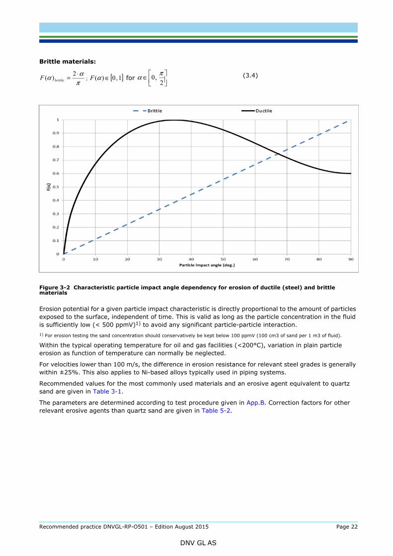


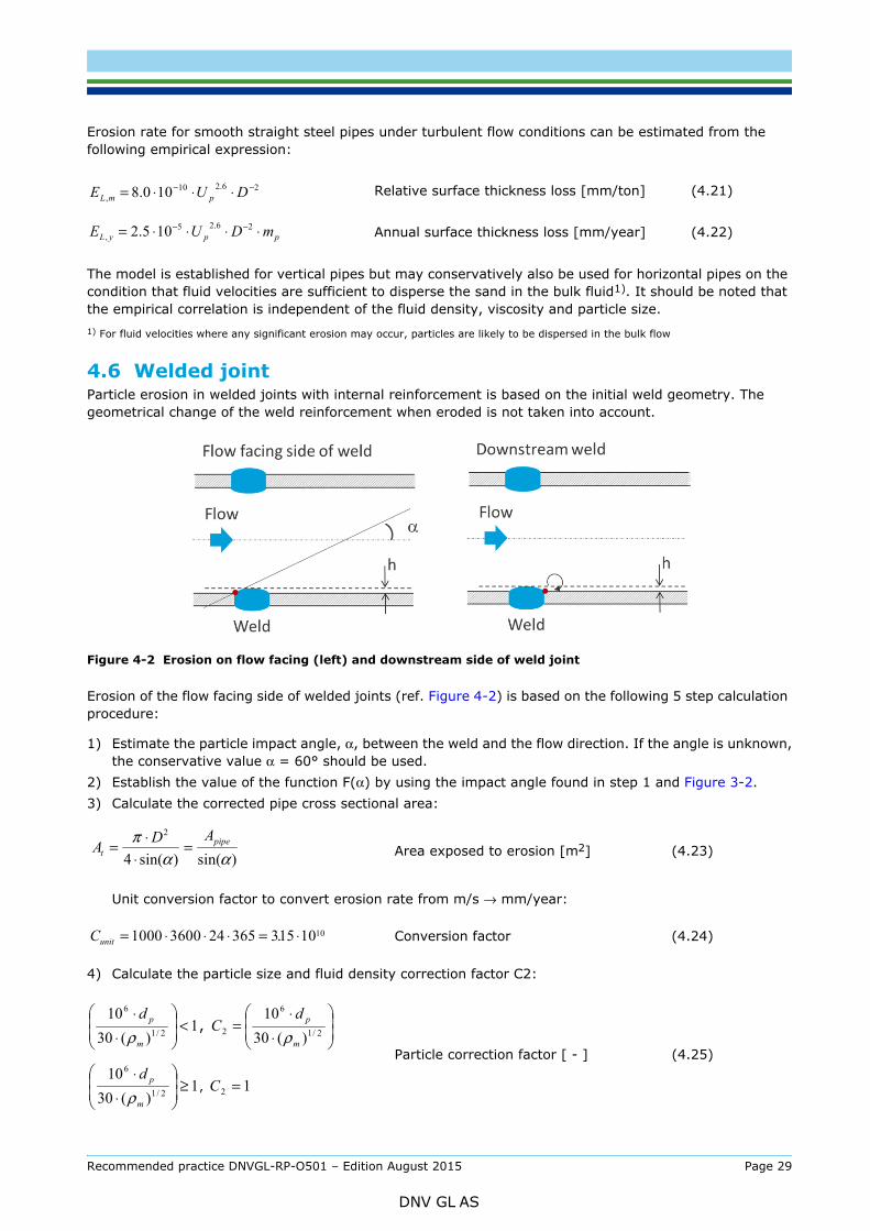


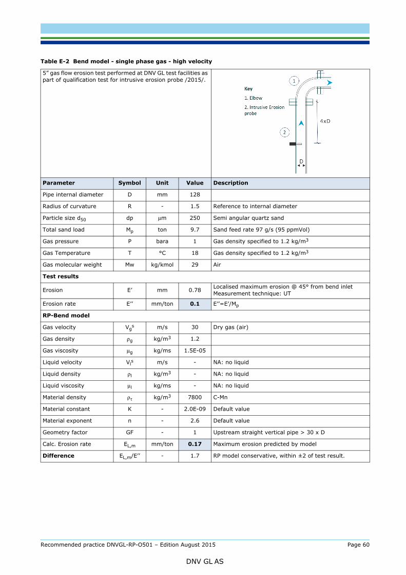


![DNVGL-RP-0043 Safety, operation and performance …rules.dnvgl.com/docs/pdf/DNVGL/RP/2017-09/DNVGL-RP-0043.pdfFor safety considerations regarding second life systems, see [7.5.1.7].](https://static.documents.pub/doc/80x56/5f9e7843ea8263465129a2ef/dnvgl-rp-0043-safety-operation-and-performance-rulesdnvglcomdocspdfdnvglrp2017-09dnvgl-rp-0043pdf.jpg)


