Bank i Kredyt 51 ( 1 ) , 2020, 1-32 Do CDS spread determinants affect the probability of default? A study on the EU banks Alessandra Ortolano*, Eliana Angelini Submitted: 3 July 2019. Accepted: 31 October 2019. Abstract The paper is an investigation of the principal variables that have affected the EU banks’ credit risk over the decade 2006–2016. In this context we adopt panel Tobit regressions in order to infer our object of analysis on the most significant CDS spread determinants illustrated by recent literature. In fact, the CDS spread should give a measure of credit risk, expressed by the probability of default. In accordance with the insertion of balance sheet, macroeconomic and market variables, we estimate the probability of default through a two-equation Merton model. Our results are analogous with the main trend of CDS spread determinants over time and contribute to continuing to consider the price of credit default swaps as a good indicator of banks’ creditworthiness. Keywords: probability of default, banks, structural models, CDS spread JEL: G10, G21, G33 * G. d’Annunzio University, Department of Economic Studies; e-mail: [email protected].
Transcript
Bank i Kredyt 51(1) , 2020, 1-32
Do CDS spread determinants affect the probability of default? A study on the EU banks
Alessandra Ortolano*, Eliana Angelini
Submitted: 3 July 2019. Accepted: 31 October 2019.
AbstractThe paper is an investigation of the principal variables that have affected the EU banks’ credit risk over the decade 2006–2016. In this context we adopt panel Tobit regressions in order to infer our object of analysis on the most significant CDS spread determinants illustrated by recent literature. In fact, the CDS spread should give a measure of credit risk, expressed by the probability of default. In accordance with the insertion of balance sheet, macroeconomic and market variables, we estimate the probability of default through a two-equation Merton model. Our results are analogous with the main trend of CDS spread determinants over time and contribute to continuing to consider the price of credit default swaps as a good indicator of banks’ creditworthiness.
Keywords: probability of default, banks, structural models, CDS spread
JEL: G10, G21, G33
* G. d’Annunzio University, Department of Economic Studies; e-mail: [email protected].
A. Or tolano, E. Angel ini2
1 Introduction
Over the last decade, European banking creditworthiness has been threatened by important events, such as financial crisis (Beyer, Cœuré, Mendicino 2017), the sovereign crisis (Gourinchas, Martin, Messer 2018; Roman, Bilan 2012) and the growth of non-performing loans (Baudino, Orlandi, Zamil 2018).
In this field, the analysis of banks’ probability of default has become a non-trivial object of observation by financial regulators and academics (EBA 2017; Elizondo Flores et al. 2010).
The default probability of a bank is not just the likelihood of bankruptcy, but is also the deterioration of its creditworthiness. Consequently, it is the expression of credit risk defined as the possibility that an unexpected change in a counterparty’s creditworthiness might generate a corresponding unexpected alteration in the market value of the associated credit exposure.
The probability of default of a bank depends on its specific factors on the one hand, and on market and macroeconomic factors on the other hand.
In this context, we intend to analyse the most significant variables affecting the probability of default, adopting CDS spread determinants. Specifically, a credit default swap is a credit derivative whose aim is to protect the buyer against an event of default dealing with the issuer of the underlying asset. Consequently, its price, called the spread, should disclose the market’s credit risk perception and its determinants might explain the main variables causing the reference entity’s credit risk. In particular the CDS spread has shown a leading role in price discovery, with reference to bond markets (e.g. Coudert, Gex 2010; Norden, Weber 2007; Blanco, Brennan, Marsh 2005) and rating announcements (Finnerty, Miller, Chen 2013; Hull, Predescu, White 2004).
In more detail, as a market indicator, CDS spread has been affected by high volatility, so we guess more accurate information might be given by the probability of default. Furthermore, the latter is implied in CDS spread and is an expression of credit risk. In accordance with the correlation between these two variables, we observe the influence of CDS spread determinants. Specifically, the related literature spans from accounting variables to market and general variables (Samaniego-Medina et al. 2016). In particular, contemporary research is developing in the study of systemic risk: general factors, indeed, seem to be more crucial than firm specific ones (Ejsing, Lemke 2011; Berndt, Obreja 2010).
In this paper, the EU banks’ credit risk is analysed over the period 2006–2016. In particular, the study consists of a two-step analysis: in the first part, there is a calculation of the probability of default on a sample of 40 banks through a two-equation Merton model. This choice is consistent with the intention to estimate this variable under both firm specific and market perspectives. The second part deals with an investigation of the relationship between the estimated probability of default and the main CDS spread determinants: this inferential study is made by the implementation of Tobit regressions for panel data. Specifically, first we present a model for the whole period and then we distinctly analyse two sub-periods (namely 2009–2012 and 2013–2016) in order to focus our attention respectively on the sovereign debt crisis and on the NPL crisis.
Our contribution is twofold: an analysis the main variables affecting the EU banks’ credit risk over time and a verification of analogies between the determinants causing the probability of default and CDS spread in order to assess if the latter is still a good indicator of banking credit risk.
Do CDS spread determinants affect the probability of default?... 3
2 Literature review
2.1 The estimation of the probability of default
There are various macro-categories of models to estimate the probability of default in order to measure credit risk.
In this paper we adopt a model belonging to the class of structural models. They are called in this way because they base the estimation of the probability of default of a company on the value of assets, on the value of debt and on the assets’ volatility. Furthermore, structural models take inspiration from contingent claim analysis, and more specifically, from options theory (Black, Scholes 1973).
The two benchmarks are the Merton model (Merton 1974) and the KMV model (Kealhofer 1993; McQuown 1993; Vasicek 1984).
In particular, the Merton model is based on the intuition that the insolvency of a company takes place when the asset value is lower than the value of liabilities: if the investments made through the borrowed capital are lower than the expectations, there will be a loss in the equity.
The KMV model, benefiting from contingent claim analysis too, assumes that the value of shares is equivalent to the price of a call option on the value of an enterprise, with the same maturity of debt and with a strike price equal to the face value of debt repayment; in addition, the model obtains the probability of default starting from the calculus of the distance-to-default variable.
Structural models have been adopted and improved by a very large strand of literature, even recently. For example, Switzer, Tu and Wang (2018), in a study on the relation between corporate governance and default risk for 28 different countries outside North America during the post-financial crisis, measure the risk of default both through Merton-type five-year default probability and through CDS spread.
Blanc-Brude and Hasan (2016) develop a structural credit risk model that relies on cash flow data in order to derive credit risk metrics; the model, implemented through project finance debt, appears useful for illiquid assets, for which a time series of prices is not observable, and provides a clear link between an asset’s fundamental characteristic and its risk profile.
Erlenmaier and Gersbach (2014), using a Merton model framework, study the relationship between default probabilities and default correlation among two firms, finding that correlation grows if the former rises.
Da and Gao (2010), criticizing Vassalou and Xing (2004), study the relationship between the stock market and default risk, measured through a default likelihood indicator derived from structural models. They find that the abnormal returns of risky stocks depend on short-term return reversals due to liquidity shock triggered by clientele change.
Other well-known categories of models are the scoring and the VaR models.The scoring models assign a number, namely a score, that expresses the default probability
of a firm. The most famous scoring model is Altman’s Z-score (Altman 1968; 1993; 2013), which derives the score through financial ratios.
VaR (i.e. value at risk) models allow to measure the market risk associated with a financial asset. It represents the maximum possible loss arising from the detention of a financial asset over a given time horizon and with a specified level of confidence or probability (e.g. Changqing, Yanlin, Mengzhen 2015; Abad, Benito 2013).
A. Or tolano, E. Angel ini4
2.2 CDS spread determinants
Below we illustrate the main recent contributions of literature on CDS spread determinants through the observation of balance sheet, market and macroeconomic variables.
Benbouzid, Leonida and Mallick (2018) suggest that CDS spread is driven by asset quality, liquidity and operations income ratio; they also check for bank size, finding a non-monotonic impact on CDS spread. Moreover, they estimate the level of bank size that minimizes the CDS spreads and find that financial institutions that grow beyond this threshold are subject to higher credit risk, implying that small and medium-sized banks are safer than large ones. In this context, they also highlight the “too- -big-to-fail” phenomenon before the onset of the financial crisis.
Alexandre, Guillemin and Refait-Alexandre (2016) study the impact of banks’ disclosure on the evolution of the related CDS spreads during the Eurozone sovereign debt crisis. They show the importance of information in terms of reduction of risk premium, since specific disclosure about sovereign exposure has a negative impact on CASC (cumulative abnormal CDS spread change); in contrast, they demonstrate that broad information positively influences CASC.
De Vincentiis (2014) compares the riskiness of global systemically important banks (G-SIB) with the no-SIBs, studying their respective CDS spreads. During a crisis period she finds the significance of the bank-specific variables (dimensions, profitability and capital stability) on the one hand, and on the other hand, the significance of the country risk, measured by sovereign CDS spreads for both kinds of banks.
Li and Zinna (2014), observing sovereign and bank CDS term structures, distinguish between the influence of systemic and sovereign risk on the banking variables, finding the highest level of systemic risk for Spain and Italy in absolute value; in a relative sense, in contrast, the most important component of risk for the banks of these countries is their respective sovereign risk, since their assets are mostly related to their home countries.
Hewavitharana and Rahmqvist (2011) examine the determinants of CDS spreads through leverage, stock return, volatility and interest rate. In a volatile context, they find a positive relationship between interest rate and CDS spreads and a negative relationship between the latter and leverage. The first relationship could be explained by the fact that in a context of economic distress, a firm is unable to meet its short-term debt payments; the second, on the other hand, is unclear. Opposite findings are shown by Ericsson, Jacobs and Oviedo (2009) during a non-crisis period.
Demirguc-Kunt, Detragiache and Merrouche (2010) regress the changes of the active banks’ 5Y CDS spreads on the changes of some market variables and banks’ capital variables. Their results confirm the latter variables as not significant, with the exception of leverage ratio. The expected signs of risk--free interest rate and stock price volatility are confirmed, respectively, with significance and not significance.
Calice, Ioannidis and Williams (2011) focus their work on large complex financial institutions and, in a section of the paper, state the relevance of the volatility of assets with respect to the risk of default. Furthermore, they show the interconnection between the CDS market and the banking sector in a systemic risk perspective.
Alter and Schüler (2012) explain the phenomenon of “private-to-public” risk transfer in Europe: before government interventions, bank credit spreads disperse to the sovereign CDS market, but after the bailouts there is an increased influence of sovereign CDS spreads on the bank spreads.
Do CDS spread determinants affect the probability of default?... 5
Acharya, Drechsler and Schnabl (2011), observing the CDS market over the period 2007–2010, underline a “two-way” feedback between sovereign and financial credit risk in the Eurozone and show an association between the increase in the sovereign CDS and a decrease in banks’ stock returns in the post-bailout period. Analogous conclusions dealt with by Caruana and Avdjiev (2012).
Specifically, on balance sheet indicators, Chiaramonte and Casu (2013) focus on a panel of international banks. They find that even if banks record very high levels of leverage, CDS spreads are not high as well until the outbreak of the crisis: this means that before this event, the market did not evaluate leverage as a significant factor of riskiness for banks, unlike the other sectors. Furthermore, in this study the significance of the indicator of asset portfolio quality as a predictor of default emerges.
The low explanatory power of leverage ratio for the banking sector is also shown by Düllmann and Sosinska (2007) and Kalemli-Ozcan, Soresen and Yesiltas (2011).
More recently Li and Fu (2017) carry out an analysis on CDS spread determinants and find that market value indicators (Tobin’s Q, stock market returns and interest rate), appear to be more important than book value indicators (i.e. ROA, ROE). Their observations deal with two European countries (Germany and France) and two Asian countries (South Korea and Hong Kong).
3 Methodology
3.1 The sample
The sample is made up of 40 banks of the European Union both from the Eurozone (2 Austria, 2 Belgium, 4 Germany, 1 Finland, 4 France, 4 Greece, 2 Ireland, 6 Italy, 1 Netherlands, 2 Portugal, 1 Slovakia, 4 Spain) and outside the Eurozone (1 Czech Republic, 2 Denmark, 1 Poland, 3 Sweden)1 (see Table 1). These observation units represent the main EU banks and are derived from a wider sample, after excluding banks that have failed during the period of analysis.
3.2 The estimation of the dependent variable: the probability of default
In this section we outline the method adopted to estimate the one-year probability of default of the banks in the sample.
This is a two-equation Merton model, so it belongs to the category of structural models for credit risk assessment.
More specifically, our model borrows from Merton’s assumption of log-normal distribution of value of assets and the KMV’s solution of a two-equation model. Even if value of banking assets generally isn’t normally distributed in times of distress (like the period analysed), the estimation of the probability of default for banks is quite similar both under a log-normal and not log-normal distribution hypothesis, as demonstrated by Nagel and Purnanandam (2019).
1 Sources of data: Datastream, Orbis Bank Focus, ECB, Eurostat.
A. Or tolano, E. Angel ini6
The model is based on a system made by two unknowns: asset value and asset volatility.
( ) ( ) ( )
( )
µ T tt t 1 t 2
E 1
E = A d – L e d
= d At/Et
1d = ( ) ( )( )2ln At /L + µ + / 2 T–t
T t
2d = 1 T td
= = dri� rate [ ]( )1 i E R+
+
,2
T = 1,
t =
=
=
0.
[ ] [ ]( ) – i i M fE R R E R R
[ ] *i f iE R R market risk premium
: At Et Lt+
( )( )1/ 1EEt At assuming d= =
( ) ( )22 / 1 / 1EEttModel E Observed E Model Observed+
( ) ( )( ) ( )( )2ln At + µ – /2 T–t –lnDD
T t
L=
( ) PD DD=
[ ]( )* PD g E PD=
( ) ( ) ( ) ( ) ( ) ( ) ,6543210, ,,,,,,1* titi i t i t i t i t i t i t
PD ROE LEV TIER LOD TENYR GDP= + + + + + + +
( ) ( ) ( ) ( ) ( ) ,543210, ,,,,,* titi i t i t i t i t i t
PD LEV LOD TENYR GDP PVOL= + + + + + +
( ) ( ) ( ) ( ) ( ), 0 1 2 3 4 5 ,, , , , ,* titi i t i t i t i t i t
μ lnT = 1, t = 0. The first equation derives from Black and Scholes formula; in the second formula, equity is like
a call on the asset value and its volatility (namely its riskiness), depends on the volatility of the asset.If the equity value Et and an estimate of the equity volatility σE are known, there are two
equations with two unknowns. This system of equations does not have a closed-form solution, but numerical routines can be used to solve it.
Now it is necessary to estimate the annual equity volatility σE. The estimation is based on the historical volatility measured over the preceding exchange days (conventionally 260), calculated on daily log returns.
Iorder to solve the system, the methodology adopted proceeds as follows.First of all, the known variables at the current time t (namely: Et, σE, Lt, μ and T ) are inserted.With reference to the unknown variables, i.e. the asset value (At)
and the asset volatility (σ), we need to assign a feasible initial value.
These initial values are calculated with the following approximations:
( ) ( ) ( )
( )
µ T tt t 1 t 2
E 1
E = A d – L e d
= d At/Et
1d = ( ) ( )( )2ln At /L + µ + / 2 T–t
T t
2d = 1 T td
= = dri� rate [ ]( )1 i E R+
+
,2
T = 1,
t =
=
=
0.
[ ] [ ]( ) – i i M fE R R E R R
[ ] *i f iE R R market risk premium
: At Et Lt+
( )( )1/ 1EEt At assuming d= =
( ) ( )22 / 1 / 1EEttModel E Observed E Model Observed+
( ) ( )( ) ( )( )2ln At + µ – /2 T–t –lnDD
T t
L=
( ) PD DD=
[ ]( )* PD g E PD=
( ) ( ) ( ) ( ) ( ) ( ) ,6543210, ,,,,,,1* titi i t i t i t i t i t i t
PD ROE LEV TIER LOD TENYR GDP= + + + + + + +
( ) ( ) ( ) ( ) ( ) ,543210, ,,,,,* titi i t i t i t i t i t
PD LEV LOD TENYR GDP PVOL= + + + + + +
( ) ( ) ( ) ( ) ( ), 0 1 2 3 4 5 ,, , , , ,* titi i t i t i t i t i t
After having also inserted the Black and Scholes formulas, the following target equation has to be solved in order to minimize the sum of squared percentage differences between model values and observed values of the equity and of assets, as shown below:
2 According to CAPM (Sharpe 1963):
( ) ( ) ( )
( )
µ T tt t 1 t 2
E 1
E = A d – L e d
= d At/Et
1d = ( ) ( )( )2ln At /L + µ + / 2 T–t
T t
2d = 1 T td
= = dri� rate [ ]( )1 i E R+
+
,2
T = 1,
t =
=
=
0.
[ ] [ ]( ) – i i M fE R R E R R
[ ] *i f iE R R market risk premium
: At Et Lt+
( )( )1/ 1EEt At assuming d= =
( ) ( )22 / 1 / 1EEttModel E Observed E Model Observed+
( ) ( )( ) ( )( )2ln At + µ – /2 T–t –lnDD
T t
L=
( ) PD DD=
[ ]( )* PD g E PD=
( ) ( ) ( ) ( ) ( ) ( ) ,6543210, ,,,,,,1* titi i t i t i t i t i t i t
PD ROE LEV TIER LOD TENYR GDP= + + + + + + +
( ) ( ) ( ) ( ) ( ) ,543210, ,,,,,* titi i t i t i t i t i t
PD LEV LOD TENYR GDP PVOL= + + + + + +
( ) ( ) ( ) ( ) ( ), 0 1 2 3 4 5 ,, , , , ,* titi i t i t i t i t i t
The estimated probabilities of default are shown below in Table 1 and Figure 1.
3.3 The regression model
In this section there is an inferential analysis based on panel generalized linear models, where the dependent variable is made by the probability of default before estimated.
Since the latter is a continuous variable delimited among the interval [0; 1], we adopt the Tobit model.
Random method is used since, as demonstrated by literature (Greene 2002; Baltagi 2000; Maddala 1987), random effects Tobit regressions for thin samples give more robust estimations than fixed effects regressions.
In particular, PD* indicates the latent dependent variable in order to calculate the Tobit linear regression. Specifically:
( ) ( ) ( )
( )
µ T tt t 1 t 2
E 1
E = A d – L e d
= d At/Et
1d = ( ) ( )( )2ln At /L + µ + / 2 T–t
T t
2d = 1 T td
= = dri� rate [ ]( )1 i E R+
+
,2
T = 1,
t =
=
=
0.
[ ] [ ]( ) – i i M fE R R E R R
[ ] *i f iE R R market risk premium
: At Et Lt+
( )( )1/ 1EEt At assuming d= =
( ) ( )22 / 1 / 1EEttModel E Observed E Model Observed+
( ) ( )( ) ( )( )2ln At + µ – /2 T–t –lnDD
T t
L=
( ) PD DD=
[ ]( )* PD g E PD=
( ) ( ) ( ) ( ) ( ) ( ) ,6543210, ,,,,,,1* titi i t i t i t i t i t i t
PD ROE LEV TIER LOD TENYR GDP= + + + + + + +
( ) ( ) ( ) ( ) ( ) ,543210, ,,,,,* titi i t i t i t i t i t
PD LEV LOD TENYR GDP PVOL= + + + + + +
( ) ( ) ( ) ( ) ( ), 0 1 2 3 4 5 ,, , , , ,* titi i t i t i t i t i t
where g() represents the link function for a Tobit transformation.3
The independent variables, listed below, are balance sheet ratios, macroeconomic and market variables.
ROE – return on equity (profitability ratio),LEV – leverage ratio (capital ratio),TIER1 – Tier 1 ratio (capital ratio),LOD – loans over deposits (liquidity ratio),
3 The real dependent PD variable derives from the inverse of the link function g().
A. Or tolano, E. Angel ini8
GDP – gross domestic product annual growth,TENYR – ten year government bond yield.Below, the equation for the overall period of analysis 2006–2016 is shown:
( ) ( ) ( )
( )
µ T tt t 1 t 2
E 1
E = A d – L e d
= d At/Et
1d = ( ) ( )( )2ln At /L + µ + / 2 T–t
T t
2d = 1 T td
= = dri� rate [ ]( )1 i E R+
+
,2
T = 1,
t =
=
=
0.
[ ] [ ]( ) – i i M fE R R E R R
[ ] *i f iE R R market risk premium
: At Et Lt+
( )( )1/ 1EEt At assuming d= =
( ) ( )22 / 1 / 1EEttModel E Observed E Model Observed+
( ) ( )( ) ( )( )2ln At + µ – /2 T–t –lnDD
T t
L=
( ) PD DD=
[ ]( )* PD g E PD=
( ) ( ) ( ) ( ) ( ) ( ) ,6543210, ,,,,,,1* titi i t i t i t i t i t i t
PD ROE LEV TIER LOD TENYR GDP= + + + + + + +
( ) ( ) ( ) ( ) ( ) ,543210, ,,,,,* titi i t i t i t i t i t
PD LEV LOD TENYR GDP PVOL= + + + + + +
( ) ( ) ( ) ( ) ( ), 0 1 2 3 4 5 ,, , , , ,* titi i t i t i t i t i t
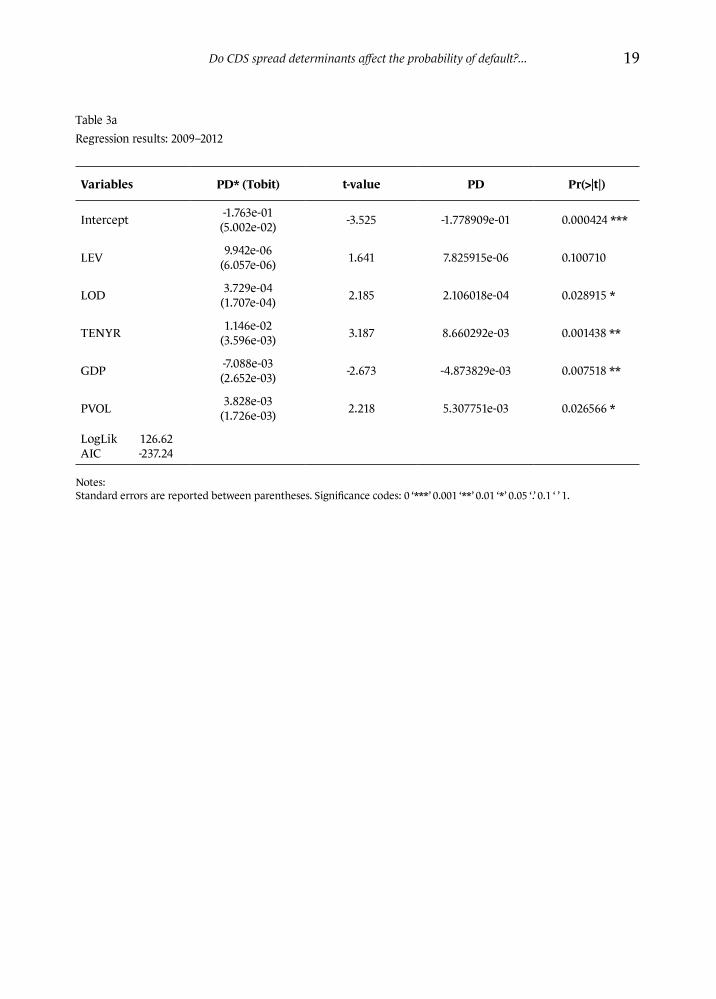
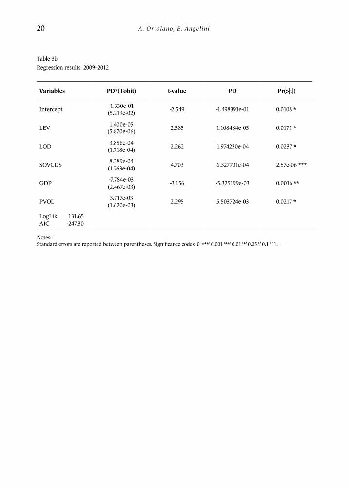
In order to analyse the impact of the Eurozone crisis on the probability of default of banks, we study the period 2009–2012, with a focus on macroeconomic and market variables. In this context, price volatility (PVOL) is introduced, while the impact of the debt crisis is controlled first through the ten year government bond yield and then with the insertion of a new variable: the sovereign CDS spread (SCDS)4 of each country of the sample.5
Below the two related equations are shown:
( ) ( ) ( )
( )
µ T tt t 1 t 2
E 1
E = A d – L e d
= d At/Et
1d = ( ) ( )( )2ln At /L + µ + / 2 T–t
T t
2d = 1 T td
= = dri� rate [ ]( )1 i E R+
+
,2
T = 1,
t =
=
=
0.
[ ] [ ]( ) – i i M fE R R E R R
[ ] *i f iE R R market risk premium
: At Et Lt+
( )( )1/ 1EEt At assuming d= =
( ) ( )22 / 1 / 1EEttModel E Observed E Model Observed+
( ) ( )( ) ( )( )2ln At + µ – /2 T–t –lnDD
T t
L=
( ) PD DD=
[ ]( )* PD g E PD=
( ) ( ) ( ) ( ) ( ) ( ) ,6543210, ,,,,,,1* titi i t i t i t i t i t i t
PD ROE LEV TIER LOD TENYR GDP= + + + + + + +
( ) ( ) ( ) ( ) ( ) ,543210, ,,,,,* titi i t i t i t i t i t
PD LEV LOD TENYR GDP PVOL= + + + + + +
( ) ( ) ( ) ( ) ( ), 0 1 2 3 4 5 ,, , , , ,* titi i t i t i t i t i t
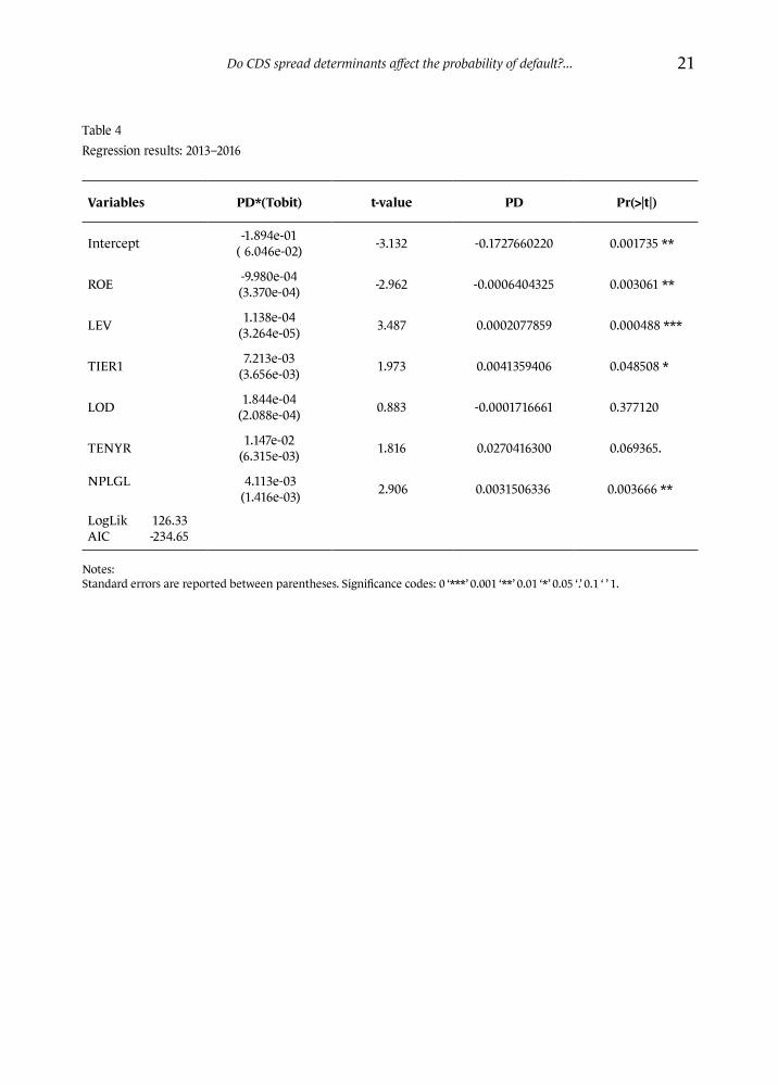
Finally, a regression for the sub-period 2013–2016, the NPL crisis years, is implemented with deeper attention to the asset quality of banks. Consequently, GDP is replaced with a new balance sheet variable: non-performing loans over gross loans ratio (NPLGL).
The related equation is the following:
( ) ( ) ( )
( )
µ T tt t 1 t 2
E 1
E = A d – L e d
= d At/Et
1d = ( ) ( )( )2ln At /L + µ + / 2 T–t
T t
2d = 1 T td
= = dri� rate [ ]( )1 i E R+
+
,2
T = 1,
t =
=
=
0.
[ ] [ ]( ) – i i M fE R R E R R
[ ] *i f iE R R market risk premium
: At Et Lt+
( )( )1/ 1EEt At assuming d= =
( ) ( )22 / 1 / 1EEttModel E Observed E Model Observed+
( ) ( )( ) ( )( )2ln At + µ – /2 T–t –lnDD
T t
L=
( ) PD DD=
[ ]( )* PD g E PD=
( ) ( ) ( ) ( ) ( ) ( ) ,6543210, ,,,,,,1* titi i t i t i t i t i t i t
PD ROE LEV TIER LOD TENYR GDP= + + + + + + +
( ) ( ) ( ) ( ) ( ) ,543210, ,,,,,* titi i t i t i t i t i t
PD LEV LOD TENYR GDP PVOL= + + + + + +
( ) ( ) ( ) ( ) ( ), 0 1 2 3 4 5 ,, , , , ,* titi i t i t i t i t i t
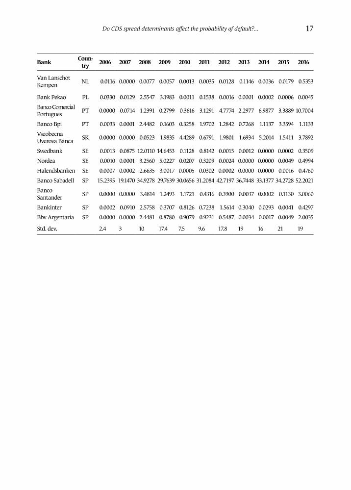
The estimated yearly probabilities of default are reported in Table 1 and shown graphically in Figure 1. The overall mean is 6.6% (Table 5a), but during the sub-periods, as could be expected, the mean values are higher, i.e. 7.6% and 8.2% respectively (Tables 6a and 7a). As concerns the variability of our results, we have shown the annual standard deviations (Table 1). In particular, we note the lowest values
4 In order to have homogeneity for the unit of measurement, the original SCDS spreads, expressed in basis points, are converted into percentage points.
5 The adoption of two distinct models is also statistically justified by the very high correlation between TENYR and SCDS covariates (+87%, see Table 9).
Do CDS spread determinants affect the probability of default?... 9
before the onset of the financial and sovereign crises, namely 2.4% and 3%, respectively, for 2006 and 2007. Starting from 2008, market volatility is reflected in the increase in the variability of our results. In particular, during the sub-period 2009–2012, the standard deviation reaches the values 17.4% and 17.8%, respectively, in 2009 and 2012: the lower values recorded in 2010 and 2011 could be explained by the government bailouts of banks; notwithstanding this, the successive regrowth of the standard deviation might be due to the “sovereign-bank risk nexus” (Fratzscher, Rieth 2019) of the European Union’s banking sector. Moreover, during the sub-period 2013–2016, the additional instability created by the NPL crisis emerges in the highest values of the variability of our estimations, with the greatest standard deviation equal to 21%, in 2015. The standard deviation of the estimated variable shows the variegated situation of credit risk in the EU: in fact, our results testify to higher values of default probability for peripheral European banks than core ones. Nevertheless, in our sample the maximum estimated probability of default (94.25%) concerns Dexia, a Belgian bank: we deem this observation unit an outlier.
4.2 The relation between the estimated probability of default and CDS determinants
In this section we illustrate the results of the regression analysis. All the outputs are shown in tables reported. Both parameters for latent (PD* ) and real (PD)
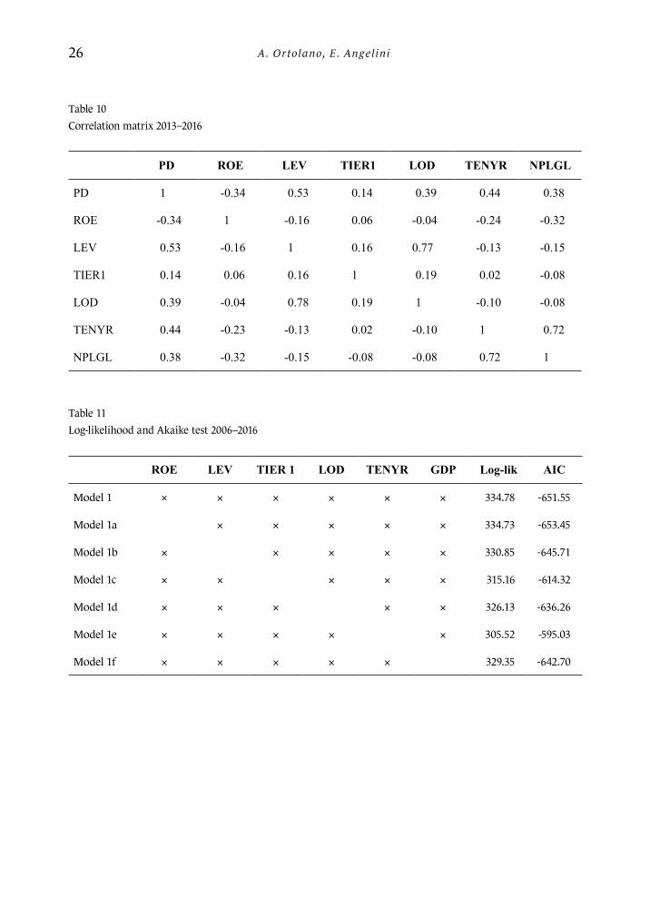
probability of default are shown.Model 1 (Table 2) deals with the period as a whole. The log-likelihood and the AIC are the best with respect to other experimented models (respectively
334.78 and -651.55, Table 11).6 Each variable of the regression is significant, with the exception of ROE. All the signs are respected; even if the positive sign of Tier 1 ratio is questionable, this is consistent with the Pearson correlation sign (+10%, Table 8). Moreover, high levels of this ratio could mislead the observants from potential criticalities of banks, in terms of credit risk (Abou-El-Sood 2016).
In particular, there are reasonable positive signs for leverage, loans over deposits and ten year government bond yields, in fact, theoretically with respect to:
LEV – the higher the liabilities of the company, the higher the probability of default,LOD – the higher the ratio, the lower the liquidity of bank, so the higher its credit risk,TENYR – the higher the government bond yields, the higher the perception of sovereign risk,
therefore the higher the growth of banks’ credit risk.The expected negative sign dealing with GDP is respected: it is intuitive that better economic
conditions represent a good framework to lessen banking sector credit risk caused by the shortage of customers’ loans repayment (Ghyasi 2016).
We also note that the highest correlation between the probability of default and the adopted covariates concern macroeconomic variables (+ 35% for TENYR and -24% for GDP, Table 8): the result confirms the relevance of these factors for banking credit risk assessment over the period analysed, as stated by recent research (Jabra, Mighri, Mansouri 2017).
6 Even if Model 1a reports a slightly better margin for the Akaike test (-1.9), the best log-lik concerns Model 1; furthermore, Model 1a has shown important criticalities in terms of multicollinearity. Moreover, we wanted to test the significance of a non-trivial ratio, like ROE.
A. Or tolano, E. Angel ini10
As concerns the analysis of the period 2009–2012, we observe the results referred to by Model 2a and Model 2b (Tables 3a and 3b).
These models provide the best results in terms of log-likelihood and Akaike test compared to other ones (Table 12). In particular, Model 2b seems to be even better than Model 2a (the referred values are respectively 131.65 and -247.30).
As already mentioned, in this period of observation there is more focus on the covariates most representative of the systemic risk, such as TENYR, SCDS spread and PVOL (Tamakoshi, Hamori 2013). These variables are the most correlated with the probability of default (respectively 44%, 42% and 50%, Table 9).
The results of the two regressions confirm the expected signs. In particular the positive sign for the government bonds, already discussed, is interesting as well as for:
– PVOL: the higher the stock volatility, the higher the credit risk transmitted by the market to banks;
– SCDS: the higher the spread, the higher the market perception of sovereign risk, so the higher the transfer of riskiness to the banking sector.
In particular, the sovereign CDS spread variable is the most significant in the analysis for this sub--period: as demonstrated (Avino, Cotter 2014) during the Eurozone debt crisis, the SCDS spread has a leading role in the discovery of banking credit risk.
Finally, as concerns Model 3 (Table 4), we focus our attention on the specific conditions of banks, with more regard to the balance sheet ratios and on the issue of NPLs.
In particular, GDP is replaced with the non-performing loans on gross loans ratio. This choice is justified by the fact that during the period analysed there is greater attention on the asset quality of banks. Meanwhile, the observation of sovereign risk and of the general level of liquidity is still relevant; in this sense we believe that it is important to also insert the TENYR variable. Consequently, this model shows better results in terms of log-lik and AIC (respectively 126.33 and -234.65) compared to Model 3a (Table 13).7
All the signs presented in the correlation matrix (Table 10) are confirmed. In particular, the new covariate is positively correlated with the probability of default by 38%: obviously the higher the percentage of NPL, the higher the riskiness of the bank. Specifically, the regression has shown a significant output for this variable.
We also note the very high significance of the leverage ratio. These results confirm the negative relation between the latter and the NPL ratio (Kashif et al.
2016); furthermore, we show the necessity to consider the quality of loans assets under a systemic point of view, as the variable is correlated with macroeconomic variables (Gila-Gourgoura, Nikolaidou 2017; Serwa 2016), like interest rates (Table 10).
5 Conclusions
This paper has investigated credit risk in the EU banking sector. To this purpose, we have inferred probability of banks’ default on CDS spread determinants through a two-step analysis: we have first estimated the dependent variable and then implemented Tobit panel regressions.
7 Even if Model 1 shows better results in terms of log-likelihood and Akaike test in relation to Model 3, it is not consistent with the object of research for the period 2013–2016 and it is also biased by multicollinearity among the covariates.
Do CDS spread determinants affect the probability of default?... 11
The probabilities of default have been estimated through a structural model: this choice appears consistent with the aim of studying credit risk both from the perspectives of firms and the market.
In the regression analysis we intended to understand both the main variables affecting the probability of default over time and whether they are the same that influence the CDS spread: in this way, we wanted to see if the latter can still be considered a good indicator of banking credit risk.
Specifically, the estimation of the probability of default has shown growing values over the years, with a particular increase during the periods of crisis.
Overall, as concerns the inferential analysis, we observed the influence of some variables related to CAMELS factors (Chodnicka-Jaworska, Jaworski 2017) and, analogously to recent CDS spread literature, we found a growing impact of macroeconomic and market variables during times of distress (e.g. Annaert et al. 2013).
In particular, during periods of crises, in terms of sovereign debt and NPLs respectively, the influence of country credit risk and asset quality problems appears significant.
The attention to these two aspects has been highlighted by the analysis of the referred periods (2009–2012 and 2013–2016 respectively), through the insertion of two explanatory variables: sovereign CDS spread variable (SCDS) and non-performing loans over equity (NPLGL).
The choice of the SCDS variable is due to the linkage of macroeconomic and policy uncertainty to the banking sector: as stated by academics, this is especially true for countries affected by the sovereign debt crisis (Drago, Di Tommaso, Thornton 2017; Yu 2017).
As concerns the study of the period 2013–2016, the adoption of NPLGL allows to observe the impact of the relation between asset quality and the capital structure of banks. This fact is particularly interesting since, as demonstrated (Bonaccorsi di Patti et al. 2014), in time of distress a high level of leverage ratio reduces banks’ resilience: the worsening of assets due to macroeconomic factors becomes more destabilising if the level of equity is too low with respect to debt. This issue is also pivotal from an economic point of view, as credit risk due to NPLs, could reduce the lending activity of banks (Cucinelli 2015).
Definitively, we deem that the credit default swap price can still be considered a good indicator of banks’ credit risk, despite the volatility caused by the speculative use of this derivative. As shown throughout the paper, its determinants have had an analogous impact on the default probability.
As concerns the perspectives for new research, the insight into banking probability of default could be proceeded by analysing credit risk from a systemic perspective (Giglio, Kelly, Pruitt 2016; Black et al. 2016), with a special focus on asset quality (Bottazzi, De Sanctis, Vanni 2016). In this context we believe it would be interesting to put more attention on the study of NPLs, finding out their main determinants and the possible strategies to reduce banking credit risk (Bruno, Iacoviello, Lazzini 2015). Moreover, as the European banking sector is characterized by linkages in terms of both sovereign and financial exposures, the research may be improved with other methodologies, such as network analysis (Westphal 2015).
A. Or tolano, E. Angel ini12
References
Abad P., Benito S. (2013), A detailed comparison of value at risk estimates, Mathematics and Computers in Simulation, 94, 258–276. Abou-El-Sood H. (2016), Are regulatory capital adequacy ratios good indicators of bank failure? Evidence from US banks, International Review of Financial Analysis, 48(C), 292–302.Acharya V.V., Drechsler I., Schnabl P. (2011), A Pyrrhic victory? Bank bailouts and sovereign credit risk, Working Paper, 17136, NBER.Alexandre H., Guillemin F., Refait-Alexandre C. (2015), Disclosure, banks CDS spreads and the European sovereign crisis, Working Paper, 10, CRESE.Alter A., Schüler Y.S. (2012), Credit spread interdependencies of European states and banks during the financial crisis, Journal of Banking and Finance, 36(12), 3444–3468. Altman E. (1968), Financial ratios, discriminant analysis and the prediction of corporate bankruptcy, Journal of Finance, 23, 589–609.Altman E. (1993), Corporate Financial Distress and Bankruptcy, John Wiley & Sons.Altman E. (2013), Predicting financial distress of companies: revisiting the Z-Score and ZETA models, Handbook of Research Methods and Applications in Empirical Finance.Annaert J., De Ceuster M., Van Roy P., Vespro C. (2013), What determines euro area bank CDS spreads?, Journal of International Money and Finance, 32(C), 444–461.Avino D., Cotter J. (2014), Sovereign and bank CDS spreads: two sides of the same coin?, Journal of International Financial Markets, Institutions & Money, 32(C), 72–85.Baltagi B. (2000), Econometric Analysis of Panel Data, John Wiley and Sons.Baudino P., Orlandi J., Zamil R. (2018), The identification and measurement of non-performing assets: a cross-country comparison, FSI Insights on Policy Implementation, 7, Bank for International Settlement.Benbouzid N., Leonida L., Mallick S.K. (2018), The non-monotonic impact of bank size on their default swap spreads: cross-country evidence, International Review of Financial Analysis, 55, 226–240.Berndt A., Obreja I. (2010), Decomposing European CDS returns, Review of Finance, 14(2), 89–233.Beyer A., Coeuré B., Mendicino C. (2017), Foreword – the crisis, ten years after: lessons learnt for monetary and financial research, Economie et Statistique / Economics and Statistics, 494–496, 45–64.Black F., Scholes M. (1973), The pricing of options and corporate liabilities, The Journal of Political Economy, 81(3), 637–654.Black L., Correa R., Huang X., Zhou H. (2016), The systemic risk of European banks during the financial and sovereign debt crises, Journal of Banking & Finance, 63(C), 107–125.Blanc-Brude F., Hasan M. (2016), A structural model of credit risk for illiquid debt, The Journal of Fixed Income, 26(1), 6–19.Blanco R., Brennan S., Marsh I.W. (2005), An empirical analysis of the dynamic relation between investment–grade bonds and credit default swaps, The Journal of Finance, 60(5), 2255–2281.Bonaccorsi di Patti E., D’Ignazio A., Gallo M., Micucci G. (2014), The role of leverage in firm solvency: evidence from bank loans, Occasional Paper, 244, Bank of Italy. Bottazzi G., De Sanctis A., Vanni F. (2016), Non-performing loans, systemic risk and resilience in financial networks, LEM Working Paper Series, 08, Laboratory of Economics and Management.
Do CDS spread determinants affect the probability of default?... 13
Bruno E., Iacoviello G., Lazzini A. (2015), On the possible tools for the prevention of non-performing loans. A case study of an Italian bank, Corporate Ownership & Control, 12(3), 133–145.Calice G., Ioannidis C., Williams J. (2011), Credit derivatives and the default risk of large complex financial institutions, Working Paper, 3583, School of Management, University of Bath. Caruana J., Avdjiev S. (2012), Sovereign creditworthiness and financial stability: an international perspective, Financial Stability Review, 16, Banque de France.Changqing L., Yanlin L., Menghezen L. (2015), Credit portfolio risk evaluation based on the pair copula VaR models, Journal of Finance and Economics, 3(1), 15–30.Chiaramonte L., Casu B. (2013), The determinants of bank CDS spreads: evidence from the financial crisis, The European Journal of Finance, 19(9), 861–887.Chodnicka-Jaworska P., Jaworski P. (2017), Fundamental determinants of credit default risk for European and American banks, Journal of International Studies, 10(3), 51–63.Coudert V., Gex M. (2010), The credit default swap market and the settlement of large defaults, Working Paper, 2010-17, CEPII Research Center.Cucinelli D. (2015), The impact of non-performing loans on bank lending behavior: evidence from the Italian banking sector, Eurasian Journal of Business and Economics, 16(8), 59–71.Da Z., Gao P. (2010), Clientele change, liquidity shock, and the return of financially distressed stocks, Journal of Financial and Quantitative Analysis, 45(1), 27–48.Demirguc-Kunt A., Detragiache E., Merrouche O. (2010), Bank capital: lessons from the financial crisis, IMF Working Paper, WP/10/286.De Vincentiis P. (2014), Lo status di banca sistemica gioca un ruolo significativo? Una verifica empirica sui Cds delle maggiori banche europee, Bancaria Special Issue, 12, 12–27.Drago D., Di Tommaso C., Thornton J. (2017), What determines bank CDS spreads? Evidence from European and US banks, Finance Research Letters, 22(C), 140–145.Düllmann K., Sosinska A. (2007), Credit default swap prices as risk indicators of listed German banks, Financial Markets and Portfolio Management, 21(3), 269–292.EBA (2017), Guidelines on PD estimation, LGD estimation and the treatment of defaulted exposures, EBA/GL/2017/16, European Banking Authority.Ejsing J., Lemke W. (2011), The Janus-headed salvation: sovereign and bank credit risk premia during 2008–2009, Economics Letters, 110(1), 28–31.Elizondo Flores J.A. et al. (2010), Regulatory use of system-wide estimations of PD, LGD and EAD, FSI Award 2010 Winning Paper, Bank for International Settlements.Ericsson J., Jacobs K., Oviedo R.A. (2009), The determinants of credit default swap premia, Journal of Financial and Quantitative Analysis, 44(1), 109–132.Erlenmaier U., Gersbach H. (2014), Default correlation in the Merton model, Review of Finance, 18, 1775–1809.Finnerty J.D., Miller C.D., Chen R. (2013), The impact of credit rating announcements on credit default swap spreads, Journal of Banking & Finance, 37(6), 2011–2030.Fratzscher M., Rieth M. (2019), Monetary policy, bank bailouts and the sovereign-bank risk nexus in the euro area, Review of Finance, 23(4), 745–775.Ghyasi A. (2016), Effect of macroeconomic factors on credit risk of banks in developed and developing countries: dynamic panel method, International Journal of Economics and Financial Issues, 6(4), 937–1944.
A. Or tolano, E. Angel ini14
Giglio S., Kelly B., Pruitt S. (2016), Systemic risk and the macroeconomy: an empirical evaluation, Journal of Financial Economics, 119(3), 457–471.Gila-Gourgoura E., Nikolaidou E. (2017), Credit risk determinants in the vulnerable economies of Europe: evidence from the Spanish banking system, International Journal of Business and Economic Sciences Applied Research, 10(1), 60–71.Gourinchas P.O., Martin P., Messer T. (2018), The economics of sovereign debt, bailouts and the Eurozone crisis, mimeo, CEPR.Greene W.H. (2002), The behavior of the fixed effects estimator in nonlinear models, Working Papers, EC-02-05, Stern School of Business, New York University.Jabra W.B., Mighri Z., Mansouri F. (2017), Determinants of European bank risk during financial crisis, Cogent Economics & Finance, 5(1).Kalemli-Ozcan S., Soresen B., Yesiltas S. (2011), Leverage across firms, banks and countries, Working Paper, 17354, National Bureau of Economic Research.Kashif M. et al. (2016), Loan growth and bank solvency: evidence from the Pakistani banking sector, Financial Innovation, 22(2).Kealhofer S. (1993), Portfolio Management of Default Risk, KMV Corporation.Hewavitharana D., Rahmqvist J. (2011), Determinants of Credit Default Swap Spreads: a Regime-shifting Approach, Lund University.Hull J., Predescu M., White A. (2004), The relationship between credit default swap spreads, bond yields, and credit rating announcements, Journal of Banking & Finance, 28(11), 2789–2811. Li M.C., Fu X. (2017), Determinants of credit default swap spreads: a four-market panel data analysis, Journal of Finance and Economics, 5(1), 9–31. Li J., Zinna G. (2014), How much of bank credit risk is sovereign risk? Evidence from the Eurozone, Working Paper, 990, Bank of Italy.Maddala G. (1987), Limited dependent variable models using panel data, Journal of Human Resources, 22, 307–338.Merton R.C. (1974), On the pricing of corporate debt: the risk structure of interest rates, Journal of Finance, 29(2), 449–470.McQuown J.A. (1993), Market vs. Accounting Based Measures of Default Risk, KMV Corporation.Nagel S., Purnanandam A. (2019), Bank risk dynamics and distance to default, Working Paper, CESifo Working Paper Series, 7637, CESifo Group.Norden L., Weber M. (2009), The co-movement of credit default swap, bond and stock markets: an empirical analysis, European Financial Management, 15(3), 529–562.Roman A., Bilan I. (2012), The euro area sovereign debt crisis and the role of ECB’s monetary policy, Procedia Economics and Finance, 3, 763–768.Samaniego-Medina et al. (2016), Determinants of bank CDS spreads in Europe, Journal of Economics and Business, 86, 1–15. Serwa D. (2016), Using nonperforming loan ratios to compute loan default rates with evidence from European banking sectors, Econometric Research in Finance, 1, 47–65.Sharpe W.F. (1963), A simplified model for portfolio analysis, Management Science, 9(2), 277–293. Switzer L.N., Tu Q., Wang J. (2018), Corporate governance and default risk in financial firms over the post-financial crisis period: international evidence, Journal of International Financial Markets, Institutions & Money, 52, 196–210.
Do CDS spread determinants affect the probability of default?... 15
Tamakoshi G., Hamori S. (2013), Volatility and mean spillovers between sovereign and banking sector CDS markets: a note on the European sovereign debt crisis, Applied Economics Letters, 20(3), 262–266.Vasicek O.A. (1984), The Philosophy of Credit Valuation: the Credit Valuation Model, KMV Corporation.Vassalou M., Xing Y. (2004), Default risk in equity returns, Journal of Finance, 59, 831–868.Westphal A. (2015), Systemic risk in the European Union: a network approach to banks’ sovereign debt exposures, International Journal of Financial Studies, 3(3), 244–279.Yu S. (2017), Sovereign and bank interdependencies – evidence from the CDS market, Research in International Business and Finance, 39, 68–84.
A. Or tolano, E. Angel ini16
Appendix
Table 1Estimated 1-year probabilities of default (%)
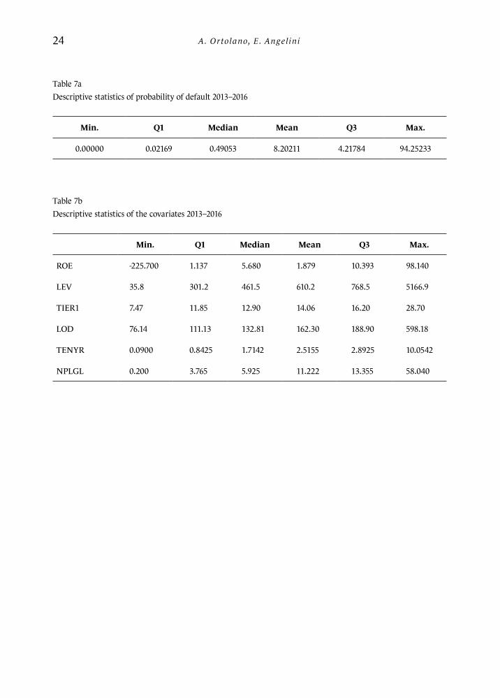
Table 7a Descriptive statistics of probability of default 2013–2016
Min. Q1 Median Mean Q3 Max.
0.00000 0.02169 0.49053 8.20211 4.21784 94.25233
Table 7bDescriptive statistics of the covariates 2013–2016
Min. Q1 Median Mean Q3 Max.
ROE -225.700 1.137 5.680 1.879 10.393 98.140
LEV 35.8 301.2 461.5 610.2 768.5 5166.9
TIER1 7.47 11.85 12.90 14.06 16.20 28.70
LOD 76.14 111.13 132.81 162.30 188.90 598.18
TENYR 0.0900 0.8425 1.7142 2.5155 2.8925 10.0542
NPLGL 0.200 3.765 5.925 11.222 13.355 58.040
Do CDS spread determinants affect the probability of default?... 25
Table 8 Correlation matrix 2006–2016
PD ROE LEV TIER1 LOD TENYR GDP
PD 1 -0.11 0.12 0.10 0.21 0.35 -0.24
ROE -0.11 1 0.20 0.21 -0.05 -0.30 0.20
LEV 0.12 0.20 1 0.01 0.25 -0.24 0.05
TIER1 0.10 0.21 0.01 1 0.06 -0.30 0.15
LOD 0.21 -0.04 0.25 0.02 1 -0.03 -0.06
TENYR 0.35 -0.30 -0.24 -0.30 -0.03 1 -0.45
GDP -0.24 0.20 0.05 0.15 -0.06 -0.44 1
Table 9Correlation matrix 2009–2012
PD LEV LOD TENYR GDP PVOL SCDS
PD 1 -0.07 0.15 0.44 -0.30 0.49 0.42
LEV -0.07 1 0.07 -0.37 0.12 -0.16 -0.42
LOD 0.15 0.07 1 -0.05 0.01 0.14 -0.02
TENYR 0.44 -0.36 -0.05 1 -0.51 0.52 0.87
GDP -0.30 0.12 0.01 -0.51 1 -0.22 -0.41
PVOL 0.50 -0.16 0.14 0.52 -0.22 1 0.42
SCDS 0.42 -0.42 -0.03 0.87 -0.41 0.42 1
A. Or tolano, E. Angel ini26
Table 10Correlation matrix 2013–2016
PD ROE LEV TIER1 LOD TENYR NPLGL
PD 1 -0.34 0.53 0.14 0.39 0.44 0.38
ROE -0.34 1 -0.16 0.06 -0.04 -0.24 -0.32
LEV 0.53 -0.16 1 0.16 0.77 -0.13 -0.15
TIER1 0.14 0.06 0.16 1 0.19 0.02 -0.08
LOD 0.39 -0.04 0.78 0.19 1 -0.10 -0.08
TENYR 0.44 -0.23 -0.13 0.02 -0.10 1 0.72
NPLGL 0.38 -0.32 -0.15 -0.08 -0.08 0.72 1
Table 11Log-likelihood and Akaike test 2006–2016
ROE LEV TIER 1 LOD TENYR GDP Log-lik AIC
Model 1 × × × × × × 334.78 -651.55
Model 1a × × × × × 334.73 -653.45
Model 1b × × × × × 330.85 -645.71
Model 1c × × × × × 315.16 -614.32
Model 1d × × × × × 326.13 -636.26
Model 1e × × × × × 305.52 -595.03
Model 1f × × × × × 329.35 -642.70
Do CDS spread determinants affect the probability of default?... 27
Table 12 Log-likelihood and Akaike test 2009–2012
ROE LEV TIER 1 LOD TENYR GDP PVOL SCDS Log-lik AIC
Model 2a × × × × × 126.62 -237.24
Model 2b × × × × × 131.65 -247.30
Model 2c × × × × × × × 126.99 -233.99
Model 1 × × × × × × 125.20 -232.40
Table 13Log-likelihood and Akaike test 2013–2016
ROE LEV TIER 1 LOD TENYR GDP NPLGL Log-lik AIC
Model 3 × × × × × × 126.33 -234.65
Model 3a × × × × × × 124.80 -231.60
Model 1 × × × × × × 131.02 -244.05
A. Or tolano, E. Angel ini28
Figure 1Estimated probabilities of default 2006–2016
1.32
663E
-05
0.00
1388
139
7.02
119E
-10
5.45
17E-
071.
0059
9E-0
52.
6809
7E-0
70.
0002
0051
73.
7127
3E-0
60.
0030
7414
17.
8371
3E-0
81.
3298
4E-0
50.
0012
8058
61.
1703
3E-0
60.
0009
3837
91.
6294
4E-0
52.
0866
9E-0
63.
2059
6E-0
51.
9232
E-05
0.00
0475
994
5.45
409E
-06
2.91
095E
-06
6.92
025E
-08
1.67
387E
-07
8.19
806E
-07
3.90
966E
-07
8.79
115E
-07
6.60
836E
-09
1.27
806E
-10
0.00
0115
578
0.00
0329
617
6.27
475E
-09
3.29
429E
-05
3.73
165E
-08
1.15
762E
-09
2.18
083E
-06
7.87
102E
-10
1.25
355E
-05
1.01
906E
-05
6.74
424E
-06
D
EXIA
KBC
KOM
ERCN
ID
EUTS
CHE
BAN
K
NAT
IXIS
CR
EDIT
AG
RIC
OLE
SO
CIET
E G
ENER
ALE
PIR
AEU
S BA
NK
BAN
K O
F IR
ELA
ND
UN
ICR
EDIT
IN
TESA
MPS
BPM
MED
IOBA
NCA UBI
V L
AN
SCH
OT
KEM
PEN
BAN
K PE
KAO
BA
NCO
BPI
BAN
CO S
ABA
DEL
L
BAN
KIN
TER
BB
V A
RGEN
TARI
ASW
EDBA
NK
NO
RD
EA
0.00
0213
565
0.00
1377
666
0.00
0359
186
5.23
393E
-06
2.14
031E
-06
8.47
594E
-06
0.00
0505
046
2.77
171E
-10
9.92
804E
-05
1.28
033E
-06
3.82
944E
-05
0.01
7088
158
6.25
311E
-05
0.00
6078
341
2.49
017E
-05
0.00
0213
019
2.56
309E
-05
1.89
099E
-05
1.21
337E
-05
3.51
196E
-05
0.00
0907
330.
0012
3729
54.
3285
7E-0
51.
5377
3E-0
93.
2843
2E-0
70.
0001
1147
4.91
892E
-09
2.81
005E
-09
2.43
22E-
100.
0001
2926
90.
0007
1444
38.
8510
5E-0
71.
9981
3E-0
8 0.19
1469
551
3.53
349E
-07
0.00
0909
881.
5501
8E-0
70.
0008
7531
91.
4410
7E-0
62.
3045
4E-0
6
0.11
3802
257
0.04
6179
011
0.10
9768
299
0.16
9895
294
0.00
9106
892
0.00
5246
553
0.04
3222
420.
0435
5838
70.
0127
7786
0.07
0703
123
0.13
6559
514
0.11
8452
714
0.03
8666
341
0.02
9150
452
0.09
9012
090.
0004
4508
1
0.09
7546
210.
0472
2261
70.
0080
8859
80.
0492
3699
0.00
0382
063
0.00
3673
67.
7015
9E-0
50.
0255
4657
10.
0123
9058
0.02
4482
329
0.00
0522
823
0.03
4813
705
0.02
5758
335
0.02
4480
772
0.03
2559
521
0.02
6634
821
0.12
5520
673
0.08
7844
044
0.17
8459
361
0.01
5107
935
0.08
1137
150.
1534
6180
73.
5920
7E-0
70.
0021
852
0.02
9154
081
0.03
8344
854
0.00
9125
383
0.06
8204
920.
1901
7743
10.
0506
5333
30.
0560
0188
20.
0553
9645
0.06
8875
466
0.06
2687
691
0.05
3925
235
0.06
7776
022
0.02
5187
976
0.00
3142
305
0.08
1553
161
0.00
2749
316
0.01
1080
833
5.68
423E
-05
0.03
1982
808
0.00
2799
474
0.00
1602
533
0.01
9834
679
0.29
7639
055
0.01
2493
072
0.00
3706
555
0.00
8779
841
0.14
6453
448
0.05
0227
240.
0300
1688
8
2009 %PD
0.00
6498
571
0.01
6466
345
0.01
0382
438
0.01
7806
282
0.00
0189
656
0.00
1129
928
0.00
0484
209
2.73
166E
-09
6.66
933E
-05
0.00
1920
108
0.00
2671
191
0.00
6125
523
0.00
8275
494
0.01
0916
668
0.01
5304
622
0.02
3322
368
0.08
2749
275
0.10
9371
541
0.05
7468
617
0.05
3566
495
0.00
9536
167
0.00
8273
441
0.00
1174
171
0.00
4828
470.
0011
0672
40.
0006
8102
11.
2650
1E-0
51.
0509
7E-0
50.
0036
1571
10.
0032
5793
50.
0442
8880
9
0.01
1720
995
0.00
8125
892
0.00
9079
305
0.00
1128
177
0.00
0207
007
5.08
041E
-06
0.02
5887
232
0.03
8252
841
0.19
6051
427
0.09
2254
817
0.00
0827
280.
0257
6037
30.
0703
4059
70.
0027
8894
70.
0045
3563
40.
0106
0162
20.
0567
6762
0.02
3332
790.
0605
0817
0.04
1189
370.
0636
9881
50.
1059
1624
1
0.20
3921
625
0.06
1934
371
0.07
8806
219
0.08
2517
924
0.03
4115
232
0.03
7700
866
0.00
5896
772
0.03
2482
864
3.51
527E
-05
0.00
1537
847
0.03
1290
719
0.01
9701
666
0.00
6790
925
0.00
4316
386
0.00
7238
179
0.00
9230
563
0.00
8141
791
0.00
3208
804
0.00
0302
039
ERST
E BA
NK
RA
IFFE
ISEN
COM
MER
ZBA
NK
UM
WEL
TBA
NK
DA
NSK
E BA
NK
JYSK
E BA
NK
ALA
ND
SBA
NKE
NBN
P PA
RIB
AS
OLD
ENBU
RG
ISCH
E
ALP
HA
BA
NK
ALL
IED
IRIS
H B
AN
K
2010 %PD 2011 %PD
2008 %PD
2006 %PD 2007 %PD
VSE
OBE
CNA
UV
ERO
VA
BA
NCA
BAN
CO C
OM
ERCI
AL
POR
TUG
UES
BAN
CO S
AN
TAN
DER
NA
T. B
AN
K O
F G
REE
CEEU
RO
BAN
K ER
GA
SIA
S
HA
LEN
DSB
AN
KEN
D
EXIA
KBC
KOM
ERCN
ID
EUTS
CHE
BAN
K
NAT
IXIS
CR
EDIT
AG
RIC
OLE
SO
CIET
E G
ENER
ALE
PIR
AEU
S BA
NK
BA
NK
OF
IREL
AN
DU
NIC
RED
IT I
NTE
SAM
PSBP
MM
EDIO
BAN
CA UBI
V L
AN
SCH
OT
KEM
PEN
BAN
K PE
KAO
BA
NCO
BPI
BA
NCO
SA
BAD
ELL
BA
NKI
NTE
R
BBV
ARG
ENTA
RIA
SWED
BAN
KN
OR
DEA
ERST
E BA
NK
RA
IFFE
ISEN
COM
MER
ZBA
NK
UM
WEL
TBA
NK
DA
NSK
E BA
NK
JYSK
E BA
NK
ALA
ND
SBA
NKE
NBN
P PA
RIB
AS
OLD
ENBU
RG
ISCH
E
ALP
HA
BA
NK
ALL
IED
IRIS
H B
AN
K
VSE
OBE
CNA
UV
ERO
VA
BA
NCA
BAN
CO C
OM
ERCI
AL
POR
TUG
UES
BAN
CO S
AN
TAN
DER
NA
T. B
AN
K O
F G
REE
CEEU
RO
BAN
K ER
GA
SIA
S
HA
LEN
DSB
AN
KEN
DEX
IAKB
CKO
MER
CNI
DEU
TSCH
E BA
NK
NAT
IXIS
CRED
IT A
GR
ICO
LESO
CIET
E G
ENER
ALE
PIR
AEU
S BA
NK
BAN
K O
F IR
ELA
ND
UN
ICR
EDIT
INTE
SAM
PSBP
MM
EDIO
BAN
CA UBI
V L
AN
SCH
OT
KEM
PEN
BAN
K PE
KAO
BAN
CO B
PI
BAN
CO S
ABA
DEL
L
BAN
KIN
TER
BB
V A
RGEN
TARI
ASW
EDBA
NK
NO
RD
EA
ERST
E BA
NK
RA
IFFE
ISEN
COM
MER
ZBA
NK
UM
WEL
TBA
NK
DA
NSK
E BA
NK
JYSK
E BA
NK
ALA
ND
SBA
NKE
NBN
P PA
RIB
AS
OLD
ENBU
RG
ISCH
E
ALP
HA
BA
NK
ALL
IED
IRIS
H B
AN
K
VSE
OBE
CNA
UV
ERO
VA
BA
NCA
BAN
CO C
OM
ERCI
AL
POR
TUG
UES
BAN
CO S
AN
TAN
DER
NA
T. B
AN
K O
F G
REE
CEEU
RO
BAN
K ER
GA
SIA
S
HA
LEN
DSB
AN
KEN
DEX
IAKB
CKO
MER
CNI
DEU
TSCH
E BA
NK
NAT
IXIS
CRED
IT A
GR
ICO
LESO
CIET
E G
ENER
ALE
PIR
AEU
S BA
NK
BAN
K O
F IR
ELA
ND
UN
ICR
EDIT
INTE
SAM
PSBP
MM
EDIO
BAN
CA UBI
V L
AN
SCH
OT
KEM
PEN
BAN
K PE
KAO
BAN
CO B
PI
BAN
CO S
ABA
DEL
L
BAN
KIN
TER
BBV
ARG
ENTA
RIA
SWED
BAN
KN
OR
DEA
ERST
E BA
NK
RA
IFFE
ISEN
COM
MER
ZBA
NK
UM
WEL
TBA
NK
DA
NSK
E BA
NK
JYSK
E BA
NK
ALA
ND
SBA
NKE
NBN
P PA
RIB
AS
OLD
ENBU
RG
ISCH
E
ALP
HA
BA
NK
ALL
IED
IRIS
H B
AN
K
VSE
OBE
CNA
UV
ERO
VA
BA
NCA
BAN
CO C
OM
ERCI
AL
POR
TUG
UES
BAN
CO S
AN
TAN
DER
NA
T. B
AN
K O
F G
REE
CEEU
RO
BAN
K ER
GA
SIA
S
HA
LEN
DSB
AN
KEN
DEX
IAKB
CKO
MER
CNI
DEU
TSCH
E BA
NK
NAT
IXIS
CRED
IT A
GR
ICO
LESO
CIET
E G
ENER
ALE
PIR
AEU
S BA
NK
BAN
K O
F IR
ELA
ND
UN
ICR
EDIT
INTE
SAM
PSBP
MM
EDIO
BAN
CA UBI
V L
AN
SCH
OT
KEM
PEN
BAN
K PE
KAO
BAN
CO B
PI
BAN
CO S
ABA
DEL
L
BAN
KIN
TER
BBV
ARG
ENTA
RIA
SWED
BAN
KN
OR
DEA
ERST
E BA
NK
RA
IFFE
ISEN
COM
MER
ZBA
NK
UM
WEL
TBA
NK
DA
NSK
E BA
NK
JYSK
E BA
NK
ALA
ND
SBA
NKE
NBN
P PA
RIB
AS
OLD
ENBU
RG
ISCH
E
ALP
HA
BA
NK
ALL
IED
IRIS
H B
AN
K
VSE
OBE
CNA
UV
ERO
VA
BA
NCA
BAN
CO C
OM
ERCI
AL
POR
TUG
UES
BAN
CO S
AN
TAN
DER
NA
T. B
AN
K O
F G
REE
CEEU
RO
BAN
K ER
GA
SIA
S
HA
LEN
DSB
AN
KEN
0.15
2394
995
0.76
4810
337
0.76
5609
615
0.42
9350
252
0.23
3826
973
0.43
5979
242
0.34
9277
561
0.12
0110
185
0.21
0389
326
0.17
8605
186
0.22
8579
562
0.19
9823
067
0.23
2742
178
0.35
5196
695
0.31
2083
663
0.29
1574
412
0.27
4157
269
0.30
0655
587
0.25
7041
895
0.29
9723
558
Do CDS spread determinants affect the probability of default?... 290.
0124
2099
40.
0170
9638
60.
8189
3123
70.
0542
1743
31.
3522
5E-0
50.
0045
9549
90.
0300
5768
20.
0523
0089
80.
0008
6295
10.
0007
9888
70.
0004
1216
40.
0286
4159
60.
0088
9314
20.
0181
6329
20.
0308
1000
40.
0317
0465
30.
4420
5186
90.
5212
7206
50.
2940
3445
80.
3991
1976
30.
1015
6597
40.
0360
9020
90.
0765
7187
10.
0242
6284
90.
0957
2647
80.
0581
1649
20.
0157
9673
60.
0249
5327
80.
0001
2778
21.
6129
1E-0
50.
0477
7436
60.
0128
4164
70.
0198
0122
50.
4271
9726
30.
0039
0022
50.
0156
1380
20.
0054
8654
11.
4548
5E-0
52.
4132
3E-0
52.
4912
8E-0
6
0.00
1495
528
0.00
0254
401
0.92
1384
261
0.00
0832
433
5.65
821E
-06
3.14
432E
-05
0.01
4103
953
0.01
2911
405
0.00
0167
351
2.85
378E
-05
2.29
414E
-06
0.02
8255
566
0.00
0111
004
0.00
0882
695
0.00
1030
218
0.00
1846
155
0.16
5831
144
0.67
2399
398
0.31
1367
513
0.32
1413
274
0.07
1892
749
0.00
6083
136
0.00
2479
408
0.00
1778
609
0.02
7722
346
0.01
3121
310.
0046
4991
10.
0046
2317
30.
0011
4598
1.49
135E
-06
0.02
2976
921
0.00
7267
626
0.01
6934
070.
3674
4849
33.
7467
6E-0
50.
0030
3983
33.
3519
E-05
1.16
733E
-05
3.35
161E
-07
1.50
015E
-07
0.00
3368
593
0.01
2340
987
0.94
2523
347
0.00
0194
221
3.78
085E
-08
1.74
705E
-05
0.00
0686
772
0.00
5066
149
0.00
6940
519
1.42
579E
-07
9.48
863E
-06
0.00
7601
067
1.14
482E
-05
0.00
0224
481
0.00
0300
279
0.00
0240
609
0.01
4238
239
0.08
0791
208
0.05
5514
841
0.32
7962
661
0.05
9233
977
0.00
7126
851
0.00
1997
292
0.00
1299
609
0.16
0134
177
0.03
0205
772
0.00
1072
781
0.00
7345
807
3.55
443E
-05
2.26
498E
-06
0.06
9876
502
0.01
1137
174
0.05
2014
456
0.33
1376
923
2.07
266E
-06
0.00
0292
968
1.65
644E
-05
3.05
894E
-09
2.81
788E
-07
1.76
001E
-10
0.00
0571
073
0.01
8268
228 0.82
6616
841.
9879
8E-0
57.
3895
E-07
0.00
0609
354
0.00
0117
252
0.00
3310
250.
0004
0841
86.
9593
8E-0
61.
0759
7E-0
60.
0075
3291
60.
0001
8135
50.
0007
7974
10.
0008
1415
20.
0004
1516
20.
5796
0074
30.
6367
7935
10.
6900
4174
90.
2468
9153
10.
1050
8878
50.
0012
5496
60.
0017
8725
40.
0008
2565
50.
0473
7907
30.
0049
1382
90.
0003
0130
30.
0026
5746
90.
0001
7910
96.
4995
5E-0
60.
0338
8908
60.
0335
9425
50.
0154
1121
0.34
2727
537
0.00
1130
112
4.08
841E
-05
4.89
076E
-05
1.50
847E
-06
4.89
544E
-05
1.62
178E
-05
0.01
2099
725
0.00
3413
915
0.78
5243
042
0.01
4266
107
3.52
814E
-05
0.05
0431
977
0.02
6059
131
0.04
1039
266
0.01
1442
752
0.00
4136
109
0.00
5588
973
0.00
4896
735
0.01
7190
697
0.02
8843
092
0.02
0650
282
0.03
5456
434
0.19
7662
973
0.34
6115
906
0.30
3453
984
0.77
5243
906
0.12
2837
677
0.07
0523
936
0.10
4554
911
0.05
0267
223
0.24
9590
027
0.17
5932
939
0.04
5595
950.
0686
2874
40.
0053
5327
14.
5300
2E-0
50.
1070
0365
70.
0111
3324
40.
0378
9164
80.
5220
2119
50.
0300
6011
60.
0042
9727
10.
0200
3549
90.
0035
0911
90.
0049
9398
90.
0047
6027
4
2016 %PD
DEX
IAKB
CKO
MER
CNI
DEU
TSCH
E BA
NK
NAT
IXIS
CRED
IT A
GR
ICO
LESO
CIET
E G
ENER
ALE
PIR
AEU
S BA
NK
BAN
K O
F IR
ELA
ND
UN
ICR
EDIT
INTE
SAM
PSBP
MM
EDIO
BAN
CA UBI
V L
AN
SCH
OT
KEM
PEN
BAN
K PE
KAO
BAN
CO B
PI
BAN
CO S
ABA
DEL
L
BAN
KIN
TER
BB
V A
RGEN
TARI
ASW
EDBA
NK
NO
RD
EA
ERST
E BA
NK
RA
IFFE
ISEN
COM
MER
ZBA
NK
UM
WEL
TBA
NK
DA
NSK
E BA
NK
JYSK
E BA
NK
ALA
ND
SBA
NKE
NBN
P PA
RIB
AS
OLD
ENBU
RG
ISCH
E
ALP
HA
BA
NK
ALL
IED
IRIS
H B
AN
K
VSE
OBE
CNA
UV
ERO
VA
BA
NCA
BAN
CO C
OM
ERCI
AL
POR
TUG
UES
BAN
CO S
AN
TAN
DER
NA
T. B
AN
K O
F G
REE
CEEU
RO
BAN
K ER
GA
SIA
S
HA
LEN
DSB
AN
KEN
DEX
IAKB
CKO
MER
CNI
DEU
TSCH
E BA
NK
NAT
IXIS
CRED
IT A
GR
ICO
LESO
CIET
E G
ENER
ALE
PIR
AEU
S BA
NK
BAN
K O
F IR
ELA
ND
UN
ICR
EDIT
INTE
SAM
PSBP
MM
EDIO
BAN
CA UBI
V L
AN
SCH
OT
KEM
PEN
BAN
K PE
KAO
BAN
CO B
PI
BAN
CO S
ABA
DEL
L
BAN
KIN
TER
BBV
ARG
ENTA
RIA
SWED
BAN
KN
OR
DEA
ERST
E BA
NK
RA
IFFE
ISEN
COM
MER
ZBA
NK
UM
WEL
TBA
NK
DA
NSK
E BA
NK
JYSK
E BA
NK
ALA
ND
SBA
NKE
NBN
P PA
RIB
AS
OLD
ENBU
RG
ISCH
E
ALP
HA
BA
NK
ALL
IED
IRIS
H B
AN
K
VSE
OBE
CNA
UV
ERO
VA
BA
NCA
BAN
CO C
OM
ERCI
AL
POR
TUG
UES
BAN
CO S
AN
TAN
DER
NA
T. B
AN
K O
F G
REE
CEEU
RO
BAN
K ER
GA
SIA
S
HA
LEN
DSB
AN
KEN
2012 %PD
2014 %PD
2013 %PD
2015 %PD
Figure 1, cont’d
A. Or tolano, E. Angel ini30
Do CDS spread determinants affect the probability of default? A study on the EU banks
Extended summary
The paper is an investigation of the principal variables that have affected the EU banks’ credit risk over the decade 2006–2016. More specifically, we intend to analyse the most significant variables affecting the probability of default, adopting CDS spread determinants. In fact, the default probability of a bank is the expression of credit risk, defined as the possibility that an unexpected change in a counterparty’s creditworthiness might generate a corresponding unexpected alteration in the market value of the associated credit exposure. The probability of default of a bank depends on its specific factors on the one hand, and on market and macroeconomic factors on the other hand. In this context, we intend to analyse the most significant variables affecting the probability of default, adopting CDS spread determinants. Specifically, a credit default swap is a credit derivative whose aim is to protect the buyer against an event of default dealing with the issuer of the underlying asset. Consequently, its price, called the spread, should disclose the market’s credit risk perception and its determinants might explain the main variables causing the reference entity’s credit risk. In particular the CDS spread has shown a leading role in price discovery, with reference to bond markets (e.g. Coudert, Gex 2010; Norden, Weber 2007; Blanco, Brennan, Marsh 2005) and rating announcements (Finnerty, Miller, Chen 2013; Hull, Predescu, White 2004). In more detail, as a market indicator, CDS spread has been affected by high volatility, so we guess more accurate information might be given by the probability of default. Furthermore, the latter is implied in CDS spread and is an expression of credit risk. In accordance with the correlation between these two variables, we observe the influence of CDS spread determinants. Specifically, the related literature spans from accounting variables to market and general variables (Samaniego-Medina et al. 2016). In particular, contemporary research is developing in the study of systemic risk: general factors, indeed, seem to be more crucial than firm specific ones (Ejsing, Lemke 2011; Berndt, Obreja 2010).
In this context our study consists of a two-step analysis: in the first part, there is a calculation of the probability of default on a sample of 40 banks through a two-equation Merton model. This choice is consistent with the intention to estimate this variable under both firm specific and market perspectives. The second part deals with an investigation of the relationship between the estimated probability of default and the main CDS spread determinants: this inferential study is made by the implementation of Tobit regressions for panel data. Specifically, first we present a model for the whole period and then we distinctly analyse two sub-periods (namely 2009–2012 and 2013–2016), in order to focus our attention respectively on the sovereign debt crisis and on the NPL crisis.
Our contribution is twofold: an analysis of the main variables affecting the EU banks’ credit risk over time and a verification of analogies between the determinants causing the probability of default and CDS spread, in order to assess if the latter is still a good indicator of banking credit risk.
Specifically, the estimation of the probability of default shows growing values over the years, with a particular increase during the periods of crisis.
Overall, as concerns the inferential analysis, we observe the influence of some variables related to CAMELS factors (Chodnicka-Jaworska, Jaworski 2017) and, analogously to recent CDS spread literature, we find a growing impact of macroeconomic and market variables during times of distress (e.g. Annaert
Do CDS spread determinants affect the probability of default?... 31
et al. 2013). In particular, during periods of crises, in terms of sovereign debt and NPLs respectively, the influence of country credit risk and asset quality problems appears significant.
Definitively, we deem that the credit default swap price can still be considered a good indicator of banks’ credit risk, despite the volatility caused by the speculative use of this derivative. As shown throughout the paper, its determinants have an analogous impact on the default probability.
As concerns the perspectives for new research, the insight into banking probability of default could be proceeded by analysing credit risk from a systemic perspective (Giglio, Kelly, Pruitt 2016; Black et al. 2016 ), with a special focus on asset quality (Bottazzi, De Sanctis, Vanni 2016). In this context we believe it would be interesting to put more attention on the study of NPLs, finding out their main determinants and the possible strategies to reduce banking credit risk (Bruno, Iacoviello, Lazzini 2015). Moreover, as the European banking sector is characterized by linkages in terms of both sovereign and financial exposures, the research may be improved with other methodologies, such as network analysis (Westphal 2015).