Do Natural Disasters Stimulate Individual Saving? Evidence ...ftp.iza.org/dp9026.pdf · developed...

DI

SC

US

SI

ON

P

AP

ER

S

ER

IE

S

Forschungsinstitut zur Zukunft der ArbeitInstitute for the Study of Labor

Do Natural Disasters Stimulate Individual Saving?Evidence from a Natural Experiment in a Highly Developed Country

IZA DP No. 9026

April 2015

Michael BerlemannMax SteinhardtJascha Tutt

Do Natural Disasters Stimulate Individual

Saving? Evidence from a Natural Experiment in a Highly Developed Country

Michael Berlemann Helmut Schmidt University, ifo and CESifo

Max Steinhardt

Helmut Schmidt University, HWWI, IZA and Lda

Jascha Tutt Helmut Schmidt University and University of Hamburg

Discussion Paper No. 9026 April 2015

IZA

P.O. Box 7240 53072 Bonn

Germany

Phone: +49-228-3894-0 Fax: +49-228-3894-180

E-mail: [email protected]

Any opinions expressed here are those of the author(s) and not those of IZA. Research published in this series may include views on policy, but the institute itself takes no institutional policy positions. The IZA research network is committed to the IZA Guiding Principles of Research Integrity. The Institute for the Study of Labor (IZA) in Bonn is a local and virtual international research center and a place of communication between science, politics and business. IZA is an independent nonprofit organization supported by Deutsche Post Foundation. The center is associated with the University of Bonn and offers a stimulating research environment through its international network, workshops and conferences, data service, project support, research visits and doctoral program. IZA engages in (i) original and internationally competitive research in all fields of labor economics, (ii) development of policy concepts, and (iii) dissemination of research results and concepts to the interested public. IZA Discussion Papers often represent preliminary work and are circulated to encourage discussion. Citation of such a paper should account for its provisional character. A revised version may be available directly from the author.

IZA Discussion Paper No. 9026 April 2015

ABSTRACT

Do Natural Disasters Stimulate Individual Saving? Evidence from a Natural Experiment in a Highly Developed Country* While various empirical studies have found negative growth-effects of natural disasters, little is yet known about the microeconomic channels through which disasters might affect short- and especially long-term growth. This paper contributes to filling this gap in the literature by studying how natural disasters affect individual saving decisions. This study makes use of a natural experiment created by the European Flood of August 2002. Using micro data from the German Socio-Economic Panel that we combine with geographic flood data, we compare the savings behavior of affected and non-affected individuals by using a difference-in-differences approach. Our empirical results indicate that natural disasters depress individual saving decisions, which might be the consequence of a Samaritan’s Dilemma. JEL Classification: Q54, D14, O16, H84 Keywords: natural disasters, floods, growth, saving behavior,

difference-in-differences approach Corresponding author: Max Steinhardt Helmut Schmidt University (HSU) Holstenhofweg 85 22043 Hamburg Germany E-mail: [email protected]

* We would like to thank Bernd Fitzenberger, Albrecht Glitz, Alkis Otto, Grischa Perino, Erik Plug, Marcel Thum, and seminar participants of the Workshop “Climate Shocks and Household Behavior” at German Institute of Economic Research (DIW Berlin), the 2014 conference of the Verein für Socialpolitik in Hamburg, the 2014 Spring Meeting of Young Economists in Vienna, the 3rd workshop on the “Economy of Climate Change” at ifo Dresden, the workshop of the Committee of Environmental and Resource Economics of the Verein für Socialpolitik, and the Research Seminar of University of Hamburg for useful comments. We also would like to thank Jan Goebel and Christine Kurka (DIW Berlin) for their data support.

mailto:[email protected]

1. Introduction

Climate change is often seen as one of the most challenging problems of our time. According

to the United Nations Human Development Report 2007/2008, “In the long run climate

change is a massive threat to human development [...]”. Against this background it does not

come as a surprise that many scientific disciplines are dealing with the causes and

consequences of climate change. This also holds true for economics, as climate-related

economic research has intensified considerably throughout the last decades. Early research

focused on the question of how regulation might contribute to a slowdown of carbon-

dioxide emissions. However, more recently the focus has changed towards forecasting the

likely economic consequences of climate change and to appropriate adaptation policies.

One consequence of climate change is the increased frequency and/or severity of certain

types of natural disasters and extreme weather events (UNISDR 2009, Thomas 2014).

Against this backdrop, there has been an increasing interest in the question of whether and

how natural disasters affect economic growth. Since the first systematic analysis of this

question was conducted by Skidmore and Toya (2002), a growing body of empirical literature

studying the growth effects of natural disasters has evolved. Most of the existing empirical

evidence concerns the short-term effects of natural disasters (see, e.g., Kahn 2005, Anbarci

et al. 2005, Bluedorn 2005, Raddatz 2007, Loayza et al. 2012, Noy 2009, Mechler 2009,

Hochrainer 2009 and Strobl 2012). The existing body of research tends to find negative

short-term growth effects of natural disasters. These negative short-term effects are more

pronounced in less developed than in high income countries. As Noy (2009) argues, this

might be due to financial constraints in reconstruction, less developed insurance markets,

and limited possibilities to run counter-cyclical fiscal policies. Much less empirical evidence is

available on the long-term growth effects of natural disasters. In their cross-sectional study

of 89 countries, the pioneering paper by Skidmore and Toya (2002) finds different results for

climatic and geologic disasters. Whereas the frequency of climatic natural disasters turns out

to have a positive effect on economic growth, geologic disasters tend to have a negative

although insignificant impact on economic growth. However, most subsequent studies have

found a negative impact of natural disasters on long-run growth (see e.g. Noy and Nualsri

2007, Raddatz 2009, Felbermayr and Gröschl 2014, and Hsiang and Jina 2014).

2

Broadly summarized, one might conclude that natural disasters, at least large ones, tend to

affect economic growth negatively, both in the short- and long-run, although the strength of

the effect depends on country characteristics and the type of disaster. Interestingly enough,

the existing empirical literature remains relatively vague with respect to the specific

channels through which natural disasters might affect long-run economic growth. Only a few

papers have engaged in attempts at uncovering these channels.1

In this paper we aim to shed additional light on one specific channel through which natural

disasters might affect economic growth: saving behavior. The savings rate is well-known to

be a decisive factor in determining per-capita income in macroeconomic models of

economic growth in closed economies. In open economies, the role of domestic saving for

economic growth is less clear, as domestic investments can also be financed by foreign

savings. However, there are reasonable theoretical arguments for why domestic saving is

also crucial in open economies. Dooley, Folkerts-Landau and Garber (2004) argue that poor

and instable countries in particular might transfer domestic savings to countries of possible

investors, thereby making expropriations of foreign investors’ capital less likely. Thus, the

transfer of domestic savings takes on the role of collateral, which encourages foreign

investments and contributes to better economic development. In a similar vein, however,

based on a well-defined theoretical model, Aghion, Comin and Howitt (2006) argue that

domestic savings play an important role in relatively poor countries that employ production

technologies far away from the actual frontier techniques. In these countries, catching up to

developed countries requires a joint venture between a foreign investor who is familiar with

the frontier technology and a domestic entrepreneur who is familiar with the local

conditions. In this scenario, domestic savings are necessary to mitigate the agency problem

which would otherwise deter the foreign investor from joining this project. The empirical

evidence that Aghion, Comin and Howitt (2006) present supports the relevance of this line of

argument. Moreover, most of the existing panel studies on the determinants of economic

growth suggest that domestic savings have a positive impact on economic growth (see, e.g.

Barro 1991, Mankiw, Romer and Weil (1992) or Islam 1995).

1 We summarize the related literature in section two of this paper.

3

In summary, we might conclude that whenever natural disasters have a systematic influence

on domestic savings behavior, medium- or even long-term economic growth will also be

affected. However, the effect of natural disasters on domestic savings is ex-ante ambiguous.

In principle natural disasters can affect individual saving behavior in different ways and

through different channels.

Saving is typically seen as a means of consumption smoothing. Naturally, the amount of

saving will increase with a corresponding increase in life expectation. Whenever natural

disasters make individuals believe that life expectations decrease, this might increase

consumption and depress saving. However, the theory of precautionary saving argues that

saving does not only serve to spread income over the life cycle, but might also serve as

insurance against uncertain events (Lusardi 1998). In this context, Roson et al. (2005) argue

that individuals might react to natural disasters by increasing their savings. Based on a

theoretical model of constant absolute risk aversion, Freeman, Keen and Mani (2003) show

that the optimal amount of precautionary saving depends positively on expected loss, and

thus on both the disaster probability and disaster loss. Natural disasters might increase

expected losses and thus increase precautionary saving. This effect should be the more

pronounced in more risk-averse individuals (Fuchs-Schündeln and Schündeln 2005).

However, it is also possible that precautionary saving is reduced as a consequence of natural

disasters. Often individuals who have suffered from catastrophic losses are supported or

even compensated by state institutions, private donations, or international aid. All these

forms of support decrease the incentives for accumulating one’s own precautionary savings.

Finally, individuals might be forced to reduce saving for a certain period of time in response

to natural disasters, due to increases in expenditures (e.g., for repairs or replacements) or

negative income shocks.

In order to further investigate the effects of natural disasters on saving behavior, we study

whether the occurrence of a large natural disaster (i.e., the flood of August 2002 in central

Europe) affected subsequent individual saving behavior in the flooded region. We base our

study on micro-level data from the German Socio-Economic-Panel (SOEP), thereby focusing

on those panel members who lived in Saxony, which was the German state that was the

most affected by the flood catastrophe. Using geo-referenced intensity-maps of the flood,

we identify two groups of individuals. The first group of individuals lived in regions of Saxony

4

that were unaffected by the flood; they serve as our control group. The second group lived

inside the flooded regions and make up our treatment group. We then apply a difference-in-

differences approach to analyze the impact of the 2002 flood on individual saving behavior.2

We find that the flood caused a significant reduction in individual savings. We also show that

this finding cannot be explained by income effects alone, and discuss the potential driving

forces behind our results.

The remainder of the paper is organized as follows. In the second section, we briefly

summarize the related empirical literature. The third section gives a brief overview on the

August 2002 flood catastrophe in central Europe, with a special emphasis on Saxony,

introduces the dataset, and explains our estimation strategy. In section four, we study the

effect of the flood catastrophe on individual saving volume, and also distinguish between the

extensive and intensive margin of the saving decision. Section five examines the potential

income effects and analyzes the individual savings rates. Section six delivers additional

robustness checks. The final section, we summarize our main results and offer concluding

remarks.

2. Related Literature

In the standard neoclassical growth model, a natural disaster destroying parts of an

economy’s capital stock and has a negative short-term impact on per-capita Gross Domestic

Product (GDP). Thus, in the very short-term perspective, natural disasters should negatively

affect the growth rate. As the economy returns to its long-term steady state, the

intermediate growth rate must exceed the long-term trend. In the long-run, the growth rate

should remain unaffected by the disaster as the economy has returned to its steady state.

Natural disasters might have an influence on long-run economic growth whenever one of

the key variables (i.e., those assumed to be exogenous in the standard neoclassical growth

2 Bechtel and Hainmueller (2011) use the August 2002 flood to analyze the impact of national aid flows on voter gratitude. Using data on electoral districts, they apply a difference-in-differences analysis to estimate the effect of disaster aid on national election outcomes. In contrast to our paper, they did not use geo-referenced information on floods, but aggregated data on flooding at the level of electoral districts. Regarding flood assistance, they assume that every district that was affected by the flood received disaster aid. They conclude that flood aid had a positive impact on the voter share of the incumbent party in the preceding election.

5

model) changes as a result of a natural disaster. The most important factors determining

steady state per-capita GDP are the savings rate (i.e., and thus investments), population

growth, human capital accumulation, and the rate of technical progress. However, to date

the empirical literature has rarely studied whether and how the occurrence of natural

disasters influences these factors. To the best of our knowledge, the only study that is

explicitly concerned with the effects of natural disasters on these growth factors is the early

study by Skidmore and Toya (2002). The authors detected no significant effect of disaster

risk (i.e., measured by the average rate of disasters which occurred throughout the sample

period of 1960-1990) on the growth of physical capital (and thus saving). The effect of

natural disasters on human capital growth and total factor productivity turns out to depend

on the type of natural disaster. While the effect of geologic disasters is negative and

insignificant, the effect of climatic disasters on both human capital accumulation and total

factor productivity is positive and significant. The authors therefore conclude that climatic

disasters have a positive impact on long-run economic growth, as climatic disasters provide

the opportunity to update capital stock and adapt new technologies. However, subsequent

literature has found little support for this hypothesis that climatic natural disasters have a

positive long-term growth effect.

Based on a life cycle expected utility model, Skidmore (2001) shows that saving should

generally increase as a result of rising expected future losses from natural disasters. While

this result does not hold when perfect insurance is available, Skidmore (2001) argues that

even in highly developed countries, disaster insurance is often unavailable due to the

combination of the low likelihood of disaster occurrence and the enormous damages to be

covered in the case of disaster events. Based on a very small dataset consisting of 15 highly

developed countries, Skidmore (2001) found that the more a country is prone to natural

disasters, the higher the aggregate saves rate.

In order to investigate how natural disasters might influence long-run growth, it is useful to

study behavioral responses to disasters at the microeconomic level. Although the existing

empirical evidence is relatively scarce, recently a number of papers have studied this issue,

although rarely in a growth context. Sawada and Shimizutani (2008) find that post-disaster

consumption behavior patterns after the Kobe earthquake depend strongly on individual

borrowing constraints. In an attempt to quantify the costs of floods in European countries,

6

Luechinger and Raschky (2009) find that individual happiness is negatively affected by flood

disasters. Berlemann (2014) finds that global hurricanes only depress happiness in the short-

run. However, hurricane risk turns out to have a strong negative impact on life satisfaction.

Page et al. (2014) find that the Brisbane flood of 2011 had a significant effect on individual

risk seeking behavior whenever an individual suffered a large loss in wealth. Cameron and

Shah (2013) conducted several field experiments with individuals affected by disasters in

rural Indonesia and find them to be more risk adverse. Taken together, this evidence

suggests that natural disasters might induce behavioral responses.

3. Background, Data and Methodology

In our analysis of behavioral responses to natural disasters, we study whether and how

individuals adjusted their saving behavior in response to a severe flood that occurred in

central Europe in summer 2002. Before we turn to the empirical analysis, we first summarize

the main facts about the flood catastrophe. We then turn to a description of the dataset and

explain the basic strategy used to identify individuals who were affected by the flood. The

section ends with an introduction of the employed empirical methodology.

3.1 The August 2002 Flood in Saxony

In July and the beginning of August 2002, central Europe experienced multiple waves of

heavy rainfall and thunderstorms. Several watercourses exhibited increased gauge stages

and the soil was saturated with water in many parts of Saxony, Bavaria, the Czech Republic,

and Austria (Löpmeier 2003). The first floods in these areas occurred between August 7 and

11, as water houses were only able to drain off above ground (GWS 2007). In the early hours

of August 12, the storm front Ilse crossed the Czech Republic and moved towards Saxony.

The overall meteorological situation in Europe during that time and the orographic

conditions in Saxony caused extreme rain as the storm front Ilse completely unloaded its

waters above eastern Germany. In the Ore Mountains, which are close to the Czech boarder,

official measures reported 312 liters of water per square meter within 24 hours (Rudolf and

Rapp 2003). This all-time German record exceeded historical precipitation levels by a factor

of four. In other central European regions, Ilse dropped between 80 and 167 liters of water

7

per square meter in a 24 hour period. In many affected regions, the water masses caused

massive direct damage.

In Saxony, the water masses caused destruction through various channels. First, small

watercourses in the Ore Mountains flooded and caused destruction on their way down to

the Elbe River. Much of the reported damage was caused by these tributaries that are

normally rather small. Second, many of the water reservoirs located in the Ore Mountains

already exhibited increased gauge stages. Traditionally the reservoirs had two functions,

drinking water storage and flood prevention for the Elbe valley. In late July, many of the

reservoirs had gauge stages close to maximum in order to provide ample fresh and drinking

water for the summer season. When the somewhat unexpected heavy rain period started,

emergency drainages became necessary in various reservoirs to prevent bursting dams. As a

consequence of one of these emergency drainages, the Weißeritz stream, which is normally

a small watercourse in the Ore Mountains, became a torrential river within a matter of

minutes and caused massive destruction in several villages including the medium-sized city

of Freital and Saxony’s capital Dresden, where the water flooded the main station and

substantial parts of the city center. Third, the specific orographic constellation of the region

from Prague to Dresden makes the Elbe River the only significant drainage for increased

water houses. Thus, the heavy rainfall at the beginning of August steadily increased the

gauge level of the Elbe River. Finally, several flood waves from the Czech Republic made

their way down the Elbe River and reached eastern Germany after this heavy rain period of

August 11 and 12. The already high gauge stages of the Elbe thus increased even further,

thereby causing severe damage to many settlement areas close to the Elbe River.

Even though the Elbe River is by far the largest watercourse that was affected by the heavy

rain, the flood catastrophe was not restricted to its surrounding areas. As mentioned earlier,

other areas such as those close to the Mulde River were also affected, and severe damage

was often caused by small tributaries such as the Weißeritz. Consequently, the flood

affected many distinct parts of Saxony.

For Germany as a whole, the Center for Research on the Epidemiology of Disasters (CRED)

reports that 330,108 people were affected and the damage totaled $11.6 billion. In these

two dimensions, the 2002 flood is Germany’s most severe natural disaster recorded in the

CRED database.

8

3.2 Household Data

For our empirical study, we used the German Socio-Economic Panel (SOEP), a panel dataset

on German households.3 The SOEP is a representative annual panel survey which started in

1984 in West Germany, and has included the areas that formerly comprised East Germany

since German Reunification in 1990. The survey contains roughly 150 questions that allow

researchers to extract information on the socio-economic infrastructure of the included

households. Among other variables, the survey includes data such as individual wealth,

income, employment, and health status. All household members above the age of 17 are

personally interviewed. In addition to a personal interview, the head of the household

answers an additional household questionnaire. The answers given to the household

questionnaire are then attributed to all household members.4

All household variables that were used in the empirical estimations were taken from the

SOEP. To identify those households that lived in flooded areas, we made use of anonymized

regional information on the residences of SOEP respondents.5 This data is considered as

highly sensitive and is subject to particular data protection regulations. We refrain from

describing all variables here, but a complete description of the employed variables can be

found in Table A1. Instead, we focus on describing those variables which served as

dependent variables in our empirical analyses. Our analysis of individual saving behavior is

based on the answers to the question:

"Do you usually have an amount of money left over at the end of the month that you can

save for larger purchases, emergency expenses or to acquire wealth? If yes, how much?"

The respondent answers this question by reporting their monthly savings amount. As we are

interested in real rather than in nominal savings, we deflate savings by the German

consumer price index and code the result as the variable S.6 In order to be able to study the

3 The SOEP data can be obtained from the SOEP Research Center located at the German Institute for Economic Research (DIW) in Berlin. 4 For a more detailed description of the SOEP survey, see Wagner et al. (2007). 5 Section 3.3 contains a detailed description of the regional data used to identify flooded regions and how it is matched to SOEP households. 6 We make use of the consumer price index (code 61111-0001) published by the German Statistical Office. Savings are expressed in € values as of year 2000.

9

https://www.diw.de/en/diw_01.c.100339.en/about_us/legal_details.html

https://www.diw.de/en/diw_01.c.100339.en/about_us/legal_details.html

extensive margin of the saving decision, we additionally construct the dummy variable SE,

which takes the value of one whenever a respondent declares to save and zero otherwise:

𝑆𝑆𝐸𝐸 = �1|𝑆𝑆 > 00|𝑆𝑆 = 0

Finally, in order to study the saving decision at the intensive margin, we construct the

variable SI. This variable is only defined for individuals who declare they save a positive

amount of money, i.e.:

𝑆𝑆𝐼𝐼 = 𝑆𝑆 | 𝑆𝑆 > 0

3.3 Definition of Treatment and Control Group using Flood Data

In 2002, the SOEP contained 23,892 people living in 12,605 households. Of these, 1,678

people (or 860 households) lived in Saxony. As Saxony was the German state most heavily

affected by the August 2002 flood, we concentrate our analysis on SOEP members living in

Saxony when the August 2002 flood occurred. Since the financial freedom of children and

adolescents is rather limited, we exclude all respondents younger than 18 from our analysis.

In our empirical analysis, we are interested in comparing savings behavior before and after

the flood occurred. We therefore exclude all respondents who were interviewed in 2002

(i.e., after the flood occurred in early August).7 Hence, the remaining 1,032 respondents

interviewed in 2002 compose our pre-disaster observations.

A crucial issue in our empirical analysis is the identification of those SOEP respondents who

lived in the flooded area and were therefore strongly affected by the 2002 flood. Not

surprisingly, the SOEP dataset does not contain a variable or question that pertains to this

issue. However, by applying a three-step procedure which we will describe in detail, we are

nevertheless able to identify Saxon SOEP respondents who lived in the area flooded in

August 2002. In the first step, we collect detailed geographic data on the flood impact in

Saxony. For this purpose, we employ a combination of two flood intensity maps. The first

map was constructed by the Saxon State Office for Environment, Agriculture and Geology on

7 As the SOEP questionnaire is primarily carried out in the first half of the year, very few observations were excluded for this reason.

10

the basis of aerial photography and hydraulic computations. The map was refined and

updated various times; we use the version dated November 2007. As this first intensity map

excludes the city of Dresden (i.e., one of the most heavily affected regions in Saxony), we

combined this map with a flood intensity map provided by the City of Dresden’s Department

for Environmental Protection. After merging the two maps, we attained one coherent

intensity map covering the whole state of Saxony.8 The combined map contains about 220

watercourses. Some 2,800 kilometers, or 11.2 percent of Saxony’s watercourses, were

affected.9 The total flooded area amounts to about 40,000 hectares.10 Roughly 20 percent of

this area is classified as settlement or infrastructural area. Figure 1 shows a graphical

representation of the employed combined intensity map. Dark areas were flooded

throughout August 2002 while areas marked in light gray indicate watercourses. The shaded

areas depict settlements.

In the second step, we localize the SOEP households within Saxony geography. Although the

standard SOEP dataset provides only information on the state level in order to protect

respondent’s data privacy, more detailed information is available at the SOEP Research Data

Center in Berlin.11 The available geographical units comprise inter alia, official municipality

keys, postal codes, and Microm neighborhood data. All of these geographical identifiers have

been available since 2000, at the latest. As the Microm neighborhood data contains the most

detailed location information, we make use of this location identifier in our analysis. The

Microm identifier localizes households by the geo-coordinates of their living places.12

In the third and final step, we match the geo-coordinates of Saxon SOEP households with the

combined flood intensity map.13 Doing so allows us to identify which adult Saxon SOEP

respondents lived inside the flooded area, and which respondents lived outside of it, when

the August 2002 flood occurred.

8 The creation of the intensity map is based on maps with a scale of 1:10,000 (in cm) and the official topographic map TK 10. For validity checks, more highly scaled maps (e.g., 1:5,000) were used in densely populated areas. 9 In total there are about 25,000 km of watercourses in Saxony. 10 About 2.2% of the total surface area of Saxony. 11 Geo-coordinates of included households can only be obtained at the research center. Less detailed geo-referenced data can be obtained and used outside the research center. 12 For additional information on geographically referenced data and the SOEP, see Hintze and Lakes (2009). 13 Flood intensity maps and geo-coordinates of Saxon SOEP respondents were matched using the open source software Quantum GIS Dufour.

11

As our treatment group, we define those respondents who lived inside the flooded area

when the flood occurred in 2002. As our control group, we make use of those respondents

identified as living outside the flooded areas.14 In order to ensure that the control group

contains exclusively unaffected SOEP respondents, we include only those individuals living at

least 500 meters away from flooded areas when the flood event occurred.15 While in the

growth context it is interesting to study the long-run flood impact, our time perspective is

somewhat limited as parts of Saxony experienced another, yet less severe flood, in spring

2006. As this would ultimately threaten our identification strategy, we restrict our post-

disaster analysis to the years between 2003 and 2005. However, this perspective

nevertheless goes well beyond the short-term growth effect of natural disasters.16 In order

to avoid potential biases through panel attrition and outmigration, which might be

interpreted as alternative behavioral responses to the disaster, we apply two additional

conditions to our sample. First, all sample respondents must have participated in the SOEP

from 2002 to 2005. Second, all sample respondents must have continuously been living in

either an area affected or unaffected by the flood. This leaves us with a treatment group of

37 persons/year observations, and a much larger control group of 995 persons/year

observations. Table I shows the summary statistics for all variables in the pre-disaster year

(2002), conditional on being a member of the treatment or control group.

14 In our study, being unaffected implies that these individuals should not have suffered directly from the flood catastrophe and therefore did not receive any financial disaster aid by private insurance companies or the state. 15 Respondents living outside the flooded areas but closer than 500 meters to such an area were excluded from the analysis. 16 Many empirical studies on the growth effects of natural disasters solely focus on the growth effects in the subsequent year.

12

Figure 1: Intensity map of flooded areas in Saxony throughout the August 2002 flood

Source: Constructed from data from the Federal Office of Cartography and Geodesy, the Department for Environmental Protection of the City of Dresden, and the Saxon State Office for

Environment, Agriculture and Geology.

13

Table I: Summary statistics for treatment and control group Year 2002 Treatment Group Control Group Variable Mean Std. Dev. Min Max N Mean Std. Dev. Min Max N Saving Volume 202.60 299.19 0 1450.90 37 268.38 425.91 0 3869.07 967 Binary Saving (SE) (Yes = 1) 0.68 0.48 0 1 37 0.68 0.47 0 1 967

Log Saving Volume (S) 3.62 2.62 0 7.28 37 3.75 2.70 0 8.26 967

Intensive Saving (SI) 5.35 0.78 4.57 7.28 25 5.53 0.94 2.80 8.26 655

Male Household Head (Yes = 1) 0.32 0.48 0 1 37 0.60 0.49 0 1 995

Age 43.03 12.98 21 74 37 48.19 16.08 18 89 995

Homeowner (Yes = 1) 0.68 0.47 0 1 37 0.42 0.49 0 1 988

Primary Education (Yes = 1) 0.06 0.23 0 1 36 0.13 0.33 0 1 980

Secondary Education (Yes = 1) 0.75 0.44 0 1 36 0.55 0.50 0 1 980

Tertiary Education (Yes = 1) 0.19 0.40 0 1 36 0.32 0.47 0 1 980

Employed (Yes = 1) 0.72 0.45 0 1 36 0.57 0.50 0 1 987

Unemployed (Yes = 1) 0.11 0.32 0 1 36 0.09 0.28 0 1 987

Non-working (Yes = 1) 0.17 0.38 0 1 36 0.34 0.47 0 1 987

Single (Yes = 1) 0.22 0.42 0 1 37 0.21 0.41 0 1 995

Married (Yes = 1) 0.70 0.46 0 1 37 0.65 0.48 0 1 995

Other (Yes = 1) 0.08 0.28 0 1 37 0.14 0.35 0 1 995

No child (Yes = 1) 0.41 0.50 0 1 37 0.49 0.50 0 1 988

1 child (Yes = 1) 0.24 0.44 0 1 37 0.25 0.43 0 1 988

2 children (Yes = 1) 0.14 0.35 0 1 37 0.21 0.41 0 1 988

3+ children (Yes = 1) 0.22 0.42 0 1 37 0.05 0.22 0 1 988

Living in Rural Area (Yes = 1) 0 0 0 1 37 0.19 0.39 0 1 955

Summary statistics for the group located inside the flooded region (i.e., treatment group) and the control group (i.e., located a minimum of 500m from the flooded region). Attribution to each group is based on geo-referenced data. Due to missing data, observations may differ across variables. The statistics are based on SOEP answers in 2002 before the flood occurred in August. A detailed description of listed variables can be found in Table AI in the appendix.

14

3.4 Estimation Strategy

The aim of our empirical analysis is to study whether and how individuals, who lived in the

flooded area when the catastrophic flood occurred, adjusted their subsequent saving behavior.

In order to study the causal effect of the flood on saving behavior, we apply a difference-in-

differences (DD) approach as described below. We hereby follow the basic framework outlined

by Angrist and Pischke (2009).

In our setting, we have two regions (1, 2); region 2 was hit by the flood in August 2002.

Moreover, we have two periods (before August 2002, after August 2002) for which we can

observe individual saving behavior.17 Given this situation, we have two potential outcomes. S1irt

is the saving of individual i in region r (1, 2) at time t (before August 2002, post 2002) if a flood

happened, and S0irt is the saving of individual i in region r at time t if no flood happened.

However, in reality, we only observe one or the other event. For example, we can see S1irt in

region 2 in 2003 but we cannot observe the counterfactual S0irt in region 2 in 2003, since region

2 was affected by the flood in August 2002. The DD setup is based on an additive structure for

potential outcomes in the no-treatment scenario:

𝐸𝐸[𝑆𝑆0𝑖𝑖𝑖𝑖𝑖𝑖| 𝑟𝑟, 𝑡𝑡] = 𝛾𝛾𝑖𝑖 + 𝜆𝜆𝑖𝑖.

We therefore assume that saving without a flood is determined by the sum of a time-invariant

regional fixed effect (𝛾𝛾𝑖𝑖) and a time effect (𝜆𝜆𝑖𝑖) that is common across regions. Let Drt be a

dummy variable for flooded regions and periods. Assuming that 𝐸𝐸[𝑆𝑆1𝑖𝑖𝑖𝑖𝑖𝑖 − 𝑆𝑆0𝑖𝑖𝑖𝑖𝑖𝑖|𝑟𝑟, 𝑡𝑡] is the

constant 𝛿𝛿, the observed saving 𝑆𝑆𝑖𝑖𝑖𝑖𝑖𝑖 can be written as:

𝑆𝑆𝑖𝑖𝑖𝑖𝑖𝑖 = 𝛾𝛾𝑖𝑖 + 𝜆𝜆𝑖𝑖 + 𝛿𝛿𝐷𝐷𝑖𝑖𝑖𝑖 + 𝜀𝜀𝑖𝑖𝑖𝑖𝑖𝑖, (1)

where 𝐸𝐸(𝜀𝜀𝑖𝑖𝑖𝑖𝑖𝑖|𝑟𝑟, 𝑡𝑡) = 0. The expected differences for the two regions are thus:

𝐸𝐸[𝑆𝑆𝑖𝑖𝑖𝑖𝑖𝑖| 𝑟𝑟 = 1, 𝑡𝑡 = 𝑝𝑝𝑝𝑝𝑝𝑝𝑡𝑡 02] − 𝐸𝐸[𝑆𝑆𝑖𝑖𝑖𝑖𝑖𝑖|𝑟𝑟 = 1, 𝑡𝑡 = 𝑝𝑝𝑟𝑟𝑝𝑝𝑝𝑝𝑟𝑟 𝐴𝐴𝐴𝐴𝐴𝐴 02] = 𝜆𝜆𝑝𝑝𝑝𝑝𝑝𝑝𝑖𝑖 02 − 𝜆𝜆𝑝𝑝𝑖𝑖𝑖𝑖𝑝𝑝𝑖𝑖 𝐴𝐴𝐴𝐴𝐴𝐴 02

17 De facto we have more than one post-treatment period. For simplicity, we explain the DD approach with two periods only.

15

and

𝐸𝐸[𝑆𝑆𝑖𝑖𝑖𝑖𝑖𝑖| 𝑟𝑟 = 2, 𝑡𝑡 = 𝑝𝑝𝑝𝑝𝑝𝑝𝑡𝑡 02] − 𝐸𝐸[𝑆𝑆𝑖𝑖𝑖𝑖𝑖𝑖|𝑟𝑟 = 2, 𝑡𝑡 = 𝑝𝑝𝑟𝑟𝑝𝑝𝑝𝑝𝑟𝑟 𝐴𝐴𝐴𝐴𝐴𝐴 02] = 𝜆𝜆𝑝𝑝𝑝𝑝𝑝𝑝𝑖𝑖 02 − 𝜆𝜆𝑝𝑝𝑖𝑖𝑖𝑖𝑝𝑝𝑖𝑖 𝐴𝐴𝐴𝐴𝐴𝐴 02 + 𝛿𝛿.

The difference between the two expected differences, the difference-in-differences estimator,

is thus 𝛿𝛿. One way to estimate equations like (1) with additional individual level covariates,

X`𝑖𝑖𝑖𝑖𝑖𝑖, is:

𝑆𝑆𝑖𝑖𝑖𝑖𝑖𝑖 = 𝛼𝛼 + 𝛾𝛾𝑡𝑡𝑟𝑟𝛾𝛾𝛾𝛾𝑡𝑡𝑖𝑖 + 𝜆𝜆𝜆𝜆𝛾𝛾𝛾𝛾𝑟𝑟𝑖𝑖 + 𝛿𝛿(𝑡𝑡𝑟𝑟𝛾𝛾𝛾𝛾𝑡𝑡𝑖𝑖 × 𝜆𝜆𝛾𝛾𝛾𝛾𝑟𝑟𝑖𝑖) + 𝛽𝛽𝑋𝑋`𝑖𝑖𝑖𝑖𝑖𝑖 + 𝜖𝜖𝑖𝑖𝑖𝑖𝑖𝑖, (2)

where year is a dummy variable that switched to 1 in the years after the flood event happened.

The dummy treat takes the value 1 for region 2 (where the flood occurred in August 2002) and 0

otherwise.

When studying saving behavior, we start out with an analysis of the overall saving volume S. As

our saving measure cannot be negative, we use the tobit approach in the first step of our

analysis. We then turn to separate analyses of the two dimensions of the savings decision: the

decision to save at the extensive and intensive margin. As the decision to save or not to save is a

binary one, we employ probit regressions for the analysis of the extensive margin of the saving

decision (SE). The decision to save at the intensive margin (SI) is analyzed based on a log-linear

model using standard OLS techniques.

We conduct all our empirical analyses with our sample of SOEP respondents that were

attributed to either the treatment or the control group. As we analyze the effect of the flood on

saving behavior in three post-disaster years, we report three different estimates (2002/03,

2002/04 and 2002/05). In order to study the stability of the derived results and to further

investigate potential factors driving our results, we conduct a number of additional estimations

in Sections Five and Six. As it is easier to understand these estimates after learning about the

main estimation results in Section Four, we explain those approaches in later sections.

16

4. Empirical Analysis of Individual Saving Behavior

Our empirical analysis of the flood’s impact on saving behavior covers three dimensions: the

effect on overall saving S, the effect on the extensive margin SE, and the effect of the intensive

margin of the saving decision SI. Thus, we estimate the difference-in-differences regression

outlined in Equation (2) using three different dependent variables. As outlined earlier, we make

use of different estimation techniques to adequately take the different characteristics of the

referring dependent variables into account. In Table 2 we report the estimation results.18 To

ease interpretation, we only report the results for the dummy variables for year and treatment,

as well as the interaction between these two dummy variables which captures the treatment

effect.19

The upper part of Table 2 reports the results of tobit models where we estimate the flood’s

impact on the latent variable S.20 We report the effect on the uncensored latent variable rather

than on the observed variable. Thus, the estimated coefficients can be interpreted as the

predicted change in desired saving levels. The estimates suggest that the flood depressed

desired saving in all three years succeeding the disaster. However, in 2003 (i.e., the first year

after the flooding), the effect is not significant. In 2004 and 2005, the effect becomes highly

significant and also increases in magnitude. Based on our estimations, the flood induced a

reduction in the latent variable of roughly 98% in 2004 and roughly 90% in 2005.21 This suggests

that the flood had a very strong and lasting effect on individual saving behavior.

The center part of Table 2 shows the results of the probit models that analyze the decision to

save at the extensive margin. Experiencing the flood had a negative impact on the decision to

save in all post-disaster years analyzed. As for the overall saving decision, the effect of the flood

is significant in the years 2004 and 2005. In order to deliver a meaningful interpretation of the

18 The number of observations across specifications varies slightly due to missing values of explanatory variables and the choice of the dependent variable. 19 Full estimation results are provided in the appendix. 20 Our dependent variable is the logarithm of total household saving S. In cases of households with zero saving, S was manually set to one and hence the logarithm of S was set to zero. 21 We compute the effect of a switch in the binary interaction term on the latent variable by: 100[exp(coefficient)-1].

17

estimated coefficients, we compute marginal effects for an individual with median

characteristics (i.e., the year and treatment dummies and the interaction term were set to 0).22

For 2004, we find the median = individual impacted by the flood had 42 percentage points lower

probability of saving any money, as compared to 2002. Even in 2005 (i.e., three years after the

disaster), flood-affected individuals are 27 percentage points less likely to save. These findings

are in line with the results from our tobit model and suggest a rather strong behavioral reaction

to the flood.

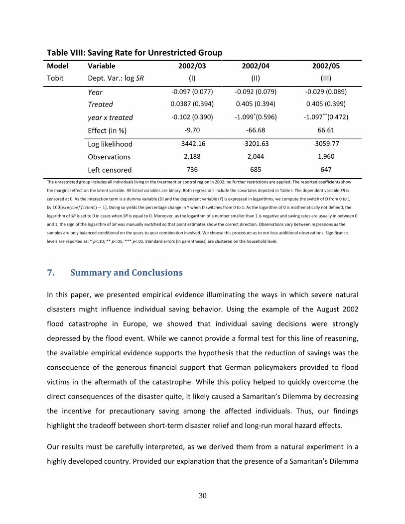
Finally, the estimates of the log linear model, as reported in the bottom part of Table 2, show

the flood’s impact at the intensive margin of the saving decision. Note that for the analysis of SI,

only those respondents that save a positive amount before the flood and in the respective post-

flood year are included in the analyses. The results differ from the earlier reported results as we

find a significant negative effect in 2003, the first post-disaster year. However, the effect

becomes insignificant in the subsequent years. This finding is likely due to several respondents

reducing their savings to zero in 2004 and 2005, as our estimates at the extensive margin have

shown.

To sum up, the results of our estimates show that the flood significantly reduced the savings of

affected individuals. While we were able to detect a response to the flood at the intensive

margin of the saving decision only in the first year after the disaster, the effect is significant at

the extensive margin of the saving decision two and three years after the disaster.

22 Results are also similar when a linear probability model is used. Estimation results are available from the authors on request.

18

Table II: Estimation Results Individual Saving Behavior Models Variable 2002/03 2002/04 2002/05 Tobit Dept. Var.: log S (I) (II) (III)

Year -0.097 (0.156) -0.120 (0.160) -0.114 (0.178)

Treated 0.145 (0.874) 0.183 (0.909) 0.154 (0.892)

year x treated -0.845 (0.775) -3.944***(1.308) -2.301**(0.982)

Effect (in %) -57,04 -98,06 -89,98

Log likelihood -4101.81 -4094.46 -4151.83

Observations 1,944 1,942 1,954

left censored 648 658 642

Probit Dept. Var.: SE

Year -0.048 (0.058) -0.051 (0.059) -0.030 (0.067)

Treated 0.120 (0.323) 0.146 (0.328) 0.125 (0.323)

year x treated -0.210 (0.293) -1.126***(0.380) -0.722**(0.302)

Marginal Effect (in %) -7.13 - 42.52 -27.51

Log pseudolikelihood -1131.64 -1137.58 -1147.59


Log linear Dept. Var.: log SI

Year -0.009 (0.041) 0.009(0.043) -0.046 (0.049)

Treated -0.088 (0.241) -0.033 (0.430) -0.176 (0.320)

year x treated -0.512***(0.189) -0.362 (0.402) -0.102 (0.268)

Effect (in %) -40.07 -30.37 -9.70

R2 0.177 0.147 0.178


All listed variables are binary. Both regressions include the covariates depicted in Table I. The dependent variable S is censored at 0. In the tobit estimates, we report

the marginal effect on the latent variable For probit estimates, we report marginal effects for a person with median characteristics. The respective year and

treatment dummies and the interaction term are all set to 0. As the interaction term is a dummy variable (D) and the dependent variable (Y) is expressed in

logarithms for the tobit and the log linear estimations, we compute the switch of D from 0 to 1 as 100[𝛾𝛾𝑒𝑒𝑝𝑝(𝑐𝑐𝑝𝑝𝛾𝛾𝑐𝑐𝑐𝑐𝑝𝑝𝑐𝑐𝑝𝑝𝛾𝛾𝑐𝑐𝑡𝑡) − 1]. Doing so yields the percentage

change in Y when D switches from 0 to 1. As the logarithm of zero is mathematically un defined, the logarithm of S is set to 0 in cases when S is equal to 0.

Observations between regressions may vary as the samples are only balanced conditional on the years-to-year combination involved. We choose this procedure as

to not lose additional observations. Significance levels are reported as: * p<.10; ** p<.05; *** p<.01. Standard errors (in parentheses) are clustered on the household

level.

19

5. Why Do Affected Individuals Reduce their Savings?

In the previous section, we presented empirical results indicating that the flood in Saxony of

August 2002 had an economically important and statistically significant negative effect on

saving behavior on those individuals who decided to stay in the disaster-affected area. As stated

in the introduction, there are several potential explanations for this finding. In this section, we

try to identify which of these explanations is the most likely driving force behind our results.

One possible explanation could be that flood-affected individuals updated their life expectancy

after the disaster and consequently changed their time preferences (see, e.g., Callen 2011,

Cassar et al. 2011). The observed reduction in savings would imply that affected individuals

expect to die earlier. Such a shift in time preferences in the context of the Elbe flooding is

unlikely. Germany is a highly developed country with relatively high protective measures (e.g.,

strict building codes) that should prevent high death tolls in face of natural disasters. Indeed,

while more than 330.000 Germans were affected by the 2002 Elbe flood, the death toll was

considerably small and amounted to 27 people (CRED). We therefore consider it very unlikely

that an update of life expectation is the driving force behind the decision to decrease saving.

A second explanation might be that decreased saving is the consequence of increased

expenditures. Individuals severely affected by the flood might have required all of their available

income to cope with the consequences of the disaster. However, one might have serious doubts

about this explanation. Significant financial aid flows were allotted to affected individuals in the

aftermath of the flood event. Affected households received governmental help, payments from

charity organizations, or insurance payments shortly after the flood. In addition, aid in kind and

neighborhood support were also substantial. For Germany as a whole, more financial aid was

available than was needed to deal with the estimated damages of the flood (Mechler and

Weichselgartner, 2003). While governmental programs could rely on a national fund of about

EUR 7.1 billion, insurance payments and charity payouts for households in Saxony alone

amounted to EUR 240 and 362 million, respectively. Governmental aid programs can be divided

20

into two programs: emergency relief and reconstruction relief.23 As the name “emergency

relief” implies, most of these payments were quickly allotted. In Saxony, nearly all requested

emergency relief funds were paid out to affected households by the end of January 2003.

Reconstruction relief, aimed at the long term support of affected homeowners, was paid out

over the whole period of the reconstruction process. Reconstruction expenses of up to 80%

were compensated by the program. By mid-2003, nearly all approved disaster relief was paid

out (Leitstelle Wiederaufbau 2003a, b). In light of these facts, it is somewhat doubtful that post-

disaster expenses forced the referring individuals to reduce their savings. Moreover, the time-

pattern we find in our estimation results does not support the enforced saving argument. A

large share of disaster-related expenses likely occurred soon after the disaster. If in fact

disaster-related expenses would have enforced decreased savings, we should observe the

savings effect to occur quickly after the flood event. However, neither total savings nor saving at

the extensive margin decreased significantly before 2004.

A third possible explanation is that the flood could have induced the observed reduction in

savings through its impact on the local labor market by reducing individual income (Vigdor 2007,

Groen and Polivka 2010, Deryugina et al. 2014a). A reduction in individual income would lead to

less disposable income and thus fewer savings. However, the flood’s short-term impact on the

economy in Saxony was rather moderate (see, e.g., Hoffmann et al. 2004, Müller and Thieken

2005, Berlemann and Vogt 2008). Moreover, the duration of the estimated effect on individual

saving behavior makes it unlikely that the reduction is caused through reduced income alone.

Household income might have temporarily declined but this effect would not have persistent

over a period of three years. For instance, Müller and Thieken (2005) report that businesses

interrupted production for two to four days after the flood.

23 Emergency relief included three subprograms. The first program aimed to support individuals and was financed by the federal state. This program allotted each person affected by the flood EUR 500, up to EUR 2000 per household. Recipients had to provide a written statement that the money would be used for replacements. The second program was similar to the first but was managed by the national government. The third program supported the emergency reconstruction of dwellings and was administered by the federal state. Owners of dwellings received up to EUR 5,000 for drainage, repairs, and maintenance, if damages were above EUR 10,000.

21

In order to formally check whether our results are primarily driven by income effects, we

compute an individual savings rates, SR, and run a number of additional regressions. Again we

estimate regressions that follow equation (2). However, we now use the savings rate as our

dependent variable. The results of the tobit regressions (Table III) are consistent with the earlier

presented results reported in Table II. As before, we report the marginal effects on the latent

saving variable. While we do not find any significant effect in the first year after the disaster, the

flood induced a significant drop in the saving rate in 2004 and 2005. Again, we calculate the

percentage change in the saving rate in order to quantify the magnitude.24 In 2004, the flood

exerted a reduction in the latent variable of about 80 percent, and still a 65 percent reduction in

2005. Given these results and our estimates from the tobit model on total saving, we conclude

that the reduction in savings were not primarily driven by a decline in income.

Table III: Estimation Results Individual Saving Rate Model Variable 2002/03 2002/04 2002/05

Tobit Dept. Var.: log SR (I) (II) (III)

Year -0.070 (0.078) -0.094 (0.079) 0.003 (0.089)

Treated 0.335 (0.440) 0.361 (0.440) 0.353 (0.442)

year x treated -0.079 (0.448) -1.657**(0.661) -1.064**(0.481)

Effect (in %) -7.60 -80.93 -65.49

Log likelihood -2962.44 -2887.03 -2956.57


Left censored 630 624 616

The reported coefficients show the marginal effect on the latent variable. All listed variables are binary. Both regressions include the covariates depicted in Table I.

The dependent variable SR is censored at 0. As the interaction term is a dummy variable (D) and the dependent variable (Y) is expressed in logarithms, we compute

the switch of D from 0 to 1 by 100[𝛾𝛾𝑒𝑒𝑝𝑝(𝑐𝑐𝑝𝑝𝛾𝛾𝑐𝑐𝑐𝑐𝑝𝑝𝑐𝑐𝑝𝑝𝛾𝛾𝑐𝑐𝑡𝑡) − 1]. Doing so yields the percentage change in Y when D switches from 0 to 1. As the logarithm of 0 is

mathematically not defined, the logarithm of SR is set to 0 in cases when SR is equal to 0. Moreover, as the logarithm of a number smaller than one is negative and

saving rates are usually in between 0 and 1, the sign of the logarithm of SR was manually switched so that the point estimates show the correct direction.

Observations vary between regressions as the samples are only balanced conditional on the years-to-year combination involved. We choose this procedure so as not

to lose additional observations. Significance levels are reported as: * p<.10; ** p<.05; *** p<.01. Standard errors (in parentheses) are clustered on the household

level.

24 As the logarithm of a number smaller than one is negative and saving rates are usually between 0 and 1, the sign of the logarithm of SR was manually switched so that point estimates were in the right direction. Moreover, as the logarithm of zero is not defined, the logarithm of SR with value 0 was manually set to 0.

22

Finally, the observed saving pattern could stem from a change in precautionary savings. As

outlined earlier, precautionary savings should be reduced whenever the perceived probability of

a disaster event and/or a disaster loss decreases. It seems counterintuitive that the occurrence

of a disaster should decrease the perceived probability of disasters occurring in the future, as

one might expect the opposite to happen instead (see, e.g., Eckel et al. 2009, Cameron and Shah

2013). However, the reduction of precautionary savings might stem from decreased perceived

disaster loss. At first glance, again there is little reason to believe that perceived disaster loss

decreases as a consequence of the occurrence of a disaster. However, it is well possible that

perceived loss is decreased by unexpected financial compensation in the aftermath of a

disaster. Given that precautionary savings are intended as insurance against unexpected

expenditures (Lusardi 1998), receipt of disaster relief can induce disaster-affected individuals to

reduce their savings.25 In particular, unprecedentedly high compensation rates might induce a

reduction in precautionary savings through moral hazard effects. This phenomenon, also known

as the Samaritan’s Dilemma (Buchanan 1975, Coate 1995) or the Charity Hazard (Raschky and

Weck-Hannemann 2007, Dobes et al. 2014), is theoretically convincing, yet, little empirical

evidence exists so far.26 As discussed earlier, the flood victims of the August 2002 event indeed

received an immense amount of financial aid (i.e., in addition to the in-kind aid and

neighborhood support already mentioned).27 Compared to disaster aid in other developed

countries, compensation was exceptionally high. Linnerooth-Bayer et al. (2001) reported that

compensation rates after disasters in several developed countries were around 40% of occurred

losses, whereas the Elbe flooding compensation rates provided almost total compensation.28

25 In a similar vein, Raschky and Weck-Hannemann (2007) argue that individuals anticipate governmental and private aid in the case of natural disasters and therefore often refrain from purchasing private disaster insurance. For a more detailed discussion, see Antwi-Boasiako (2014). 26 There is a small amount of empirical literature on the existence of the Samaritan’s Dilemma in natural hazard insurance. While the studies by Kunreuther et al. (1978) and Browne and Hoyt (2000) failed to find that government aid crowded out purchasing of private disaster insurance, the studies by van Asseldonk et al. (2002), Botzen et al. (2009), Brunette et al. (2013), Kousky et al. (2013), and Deryugina and Kirwan (2014b) report evidence that supports this argument. 27 In their analysis of the political consequences of the provided aid in the aftermath of the Elbe flood of 2002, Bechtel and Hainmueller (2011) implicitly assume high compensation rates, which is in line with our line of argument. 28 In line with this finding, Horwich (2000) reports that the governments of disaster-prone Japan traditionally provide only minimal disaster compensation in order to prevent negative incentive effects.

23

Although we have little information on pre-event expectations on disaster compensation, one

might nevertheless suspect that the extraordinary disaster aid of the Elbe flood was at least

somewhat unexpected. While the generous disaster aid surely helped to quickly overcome the

direct consequences of the flood disaster, it is also highly possible that the enormous level of aid

indeed caused a moral hazard effect that led to a reduction in self-insurance via precautionary

saving. The explanation of decreased saving by the existence of a Samaritan`s Dilemma is

further supported by the observed time-pattern in our estimation results. The strong reaction in

saving behavior happened in 2004 and 2005, and hence after most financial aid was already

been paid out.

6. Robustness Tests

In order to study the robustness of our estimation results, we present and discuss several

additional estimation results in this section.

First and most important, we study whether the assumption of parallel trends in the treatment

and control group holds true in the absence of the treatment. As the inferences in the

difference-in-differences approach are based on this assumption, we shed some light on this

issue by conducting a falsification test. This strategy estimates placebo difference-in-differences

regressions that use the same basic specification that was explained in Section Three and

employed in Section Four; the only difference is that we assume the flood occurred at some

arbitrary point in time before the actual occurrence in August 2002. Whenever the identified

differences between the treatment and the control group indeed result from the treatment, we

should find that the interaction effect between the treatment and year dummy variables is

insignificant in the placebo treatment.

24

For our placebo treatment, we assume that the flood had already occurred in August 2000 and

thus two years before it actually took place.29 All respondents questioned before August 2000

comprise the pre-treatment sample, and all respondents questioned in 2001 and before August

2002 comprise the post-treatment observations. We included only respondents which took part

in the SOEP in between 2000 and 2002. In order to construct the control and the treatment

group of the placebo treatment, we use the same procedure as described in Section 3.3. As with

the previously reported estimations, we apply the restriction that all individuals in the

treatment and control group may not have moved out of their initial living area.

The estimation results for individual saving are displayed in Table IV. In contrast to the results

reported in Section Four, the relevant interaction effect between the year and treatment

dummy variables is insignificant for both estimations (i.e., the difference between 2000 and

2001 and the difference between 2000 and 2002). Thus, we find no evidence for differing trends

between the treatment and the control group in our placebo treatment. In Table V, we show

the corresponding estimation results for individual saving rates. Again, we identify no difference

in the trends of the treatment and control group.

29 The geographic data that was used to divide the SOEP participants into the treatment and the control group was unavailable before 2000. We therefore cannot conduct placebo treatments for earlier points in time.

25

Table IV: Placebo Estimation Results Individual Saving Behavior Models Variable 2000/01 2000/02 Tobit Dept. Var.: log S (I) (II)

Year 0.007 (0.147) -0.281*(0.168)

Treated 0.178 (0.700) 0.091 (0.699)

year x treated -0.482 (0.750) 0.083 (0.419)

Effect (in %) -38.24 8.65

Log likelihood -4723.56 -4433.05

Observations 2,220 2,074

left censored 677 646


Year -0.009 (0.060) -0.104 (0.065)

Treated 0.252 (0.332) 0.205 (0.317)

year x treated -0.273 (0.315) -0.062 (0.192)

Marginal Effect (in %) -10.46 -2.25

Log pseudolikelihood -1239.32 -1207.23



Year 0.057 (0.039) -0.011 (0.046)

Treated -0.475**(0.213) -0.513**(0.200)

year x treated 0.167 (0.164) 0.143 (0.135)

Effect (in %) 18.18 15.37

R2 0.108 0.092

Observations 1338 1204

The date for the hypothetical flood event has been chosen to be August 2000. All listed variables are binary. Both regressions include the covariates depicted in Table

I. The dependent variable S is censored at 0. We report the marginal effect on the latent variable in the case of tobit estimations. For probit estimations we report

marginal effects for a person with median characteristics. The respective year and treatment dummies as well as the interaction term is set to 0. As the interaction

term is a dummy variable (D) and the dependent variable (Y) is expressed in logarithms in the case of the tobit and the log linear estimations, we compute the switch

of D from 0 to 1 as 100[𝛾𝛾𝑒𝑒𝑝𝑝(𝑐𝑐𝑝𝑝𝛾𝛾𝑐𝑐𝑐𝑐𝑝𝑝𝑐𝑐𝑝𝑝𝛾𝛾𝑐𝑐𝑡𝑡) − 1]. Doing so yields the percentage change in Y when D switches from 0 to 1. As the logarithm of 0 is mathematically un

defined, the logarithm of S is set to 0 in cases when S is equal to 0. Observations between regressions may vary as the samples are only balanced conditional on the

years-to-year combination involved. We choose this procedure as to not lose additional observations. Significance levels are reported as: * p<.10; ** p<.05; ***

p<.01. Standard errors (in parentheses) are clustered on the household level.

26

Table V: Placebo Estimation Results Individual Saving Rate Model Variable 2000/01 2000/02 Tobit Dept. Var.: log SR (I) (II)

Year -0.047 (0.077) -0.078 (0.089)

Treated 0.580 (0.426) 0.544 (0.424)

year x treated -0.599 (0.471) -0.266 (0.279)

Marginal Effect (in % ) -45,06 -23,36

Log-Likelihood -3385.83 -3224.11


Left censored 650 622 The date for the hypothetical flood event has been chosen to be August 2000. The reported coefficients show the marginal effect on the latent variable. All listed

variables are binary. Both regressions include the covariates depicted in table I. The dependent variable SR is censored at 0. As the interaction term is a dummy

variable (D) and the dependent variable (Y) is expressed in logarithms, we compute the switch of D from 0 to 1 by 100[𝛾𝛾𝑒𝑒𝑝𝑝(𝑐𝑐𝑝𝑝𝛾𝛾𝑐𝑐𝑐𝑐𝑝𝑝𝑐𝑐𝑝𝑝𝛾𝛾𝑐𝑐𝑡𝑡) − 1]. Doing so yields the

percentage change in Y when D switches from 0 to 1. As the logarithm of 0 is mathematically not defined, the logarithm of SR is set to 0 in cases when SR is equal to

0. Moreover, as the logarithm of a number smaller than one is negative and saving rates are usually in between 0 and 1, the sign of the logarithm of SR was manually

switched so that point estimates show the correct direction. Observations vary between regressions as the samples are only balanced conditional on the years-to-

year combination involved. We chose this procedure as to not lose additional observations. Significance levels are reported as: * p<.10; ** p<.05; *** p<.01.

Standard errors (in parentheses) are clustered on the household level.

Throughout the previous empirical analyses of the extensive decision to save, we defined the

referring saving variable as:

𝑆𝑆𝐸𝐸 = �1|𝑆𝑆 > 00|𝑆𝑆 = 0

Thus, even individuals with very small but positive reported savings were considered savers.

However, one might argue that in the context of disasters, a very low saving volume of only a

few Euros should not be considered as precautionary savings. As a second stability test, we

defined savers as individuals who declared that they saved more than 50 € a month, i.e.:

𝑆𝑆′𝐸𝐸 = �1|𝑆𝑆 > 50€0|𝑆𝑆 ≤ 50€

Table VI presents the corresponding estimates at the extensive margin. The results remain

qualitatively unaffected, while the calculated marginal effects slightly increase.

27

Table VI: Stability of Extensive Margin Model Variable 2002/03 2002/04 2002/05 Probit Dept. Var.: S’E (I) (II) (III)

Year 0.008 (0.059) 0.019 (0.056) -0.038 (0.066)

Treated 0.252 (0.320) 0.275 (0.325) 0.279 (0.320)

year x treated -0.431 (0.321) -1.207***(0.380) -0.747**(0.304)

Marginal Effect (in %) -16.36 -45.07 -29.12



All listed variables are binary and all regressions include the covariates depicted in Table I. Marginal effects refer to a person with median characteristics. The

respective year and treatment dummy variables and the interaction term were all set to 0. Observations between regressions vary as the samples are only balanced

conditional on the years involved. Significance levels are reported as: * p<.10; ** p<.05; *** p<.01. Standard errors (in parentheses) are clustered on the household

level.

Finally, we study whether our estimation results still hold true when we are less restrictive in

attributing respondents to the treatment and control group. Whereas previously we had only

included those respondents participated in all relevant waves of the SOEP and which not moved

out of their initial home area, we relaxed these restrictions in the estimations that are

summarized in Tables VII and VIII. Doing so generally increases the number of observations but

also leads to a more rapidly decreasing number of observations over time due to panel attrition.

The estimation results for total savings and for the extensive decision to save remain

qualitatively unchanged. The estimation results for the decision to save at the extensive margin

are also similar; however, the effect for the period between 2002 and 2003 is now insignificant.

The results for the individual saving rate again remain virtually unchanged.

28

Table VII: Estimation Results Individual Saving Behavior Unrestricted Group Models Variable 2002/03 2002/04 2002/05 Tobit Dept. Var.: log S (I) (II) (III)

Year -0.178 (0.151) -0.145 (0.158) -0.164 (0.178)

Treated 0.215 (0.787) 0.181 (0.812) 0.430 (0.817)

year x treated -0.418 (0.847) -3.139***(1.169) -2.305**(0.934)

Effect (in %) -34.16 -95.67 -90.02

Log likelihood -4705.08 -4485.79 -4299.55


left censored 752 717 676


Year -0.072 (0.055) -0.053 (0.058) -0.049 (0.066)

Treated 0.140 (0.299) 0.143 (0.302) 0.210 (0.304)

year x treated -0.110 (0.307) -0.871**(0.363) -0.704**(0.301)

Marginal Effect (in %) -3.93 -33.17 -26.66




Year -0.006 (0.038) 0.005 (0.042) -0.047 (0.049)

Treated -0.207 (0.207) -0.306 (0.313) -0.130 (0.292)

year x treated -0.274 (0.204) -0.512 (0.375) -0.236 (0.280)

Effect (in %) -23.97 -40.07 -21.02

R2 0.167 0.156 0.176


The unrestricted group includes all individuals living in the treatment or control region in 2002; no further restrictions are applied. All listed variables are binary. All

regressions include the covariates depicted in Table I. The dependent variable S is censored at 0. We report the marginal effect on the latent variable in the case of

tobit estimations. For probit estimations we report marginal effects for a person with median characteristics. The respective year and treatment dummy variables

and the interaction term are all set to 0. As the interaction term is a dummy variable (D) and the dependent variable (Y) is expressed in logarithms in the case of the

tobit and the log linear estimations, we compute the switch of D from 0 to 1 as 100[𝛾𝛾𝑒𝑒𝑝𝑝(𝑐𝑐𝑝𝑝𝛾𝛾𝑐𝑐𝑐𝑐𝑝𝑝𝑐𝑐𝑝𝑝𝛾𝛾𝑐𝑐𝑡𝑡) − 1]. Doing so yields the percentage change in Y when D

switches from 0 to 1. As the logarithm of zero is mathematically not defined, the logarithm of S is set to 0 in cases when S is equal to 0. Observations between

regressions may vary as the samples are only balanced conditional on the years-to-year combination involved. We choose this procedure as to not lose additional

observations. Significance levels are reported as: * p<.10; ** p<.05; *** p<.01. Standard errors (in parentheses) are clustered on the household level.

29

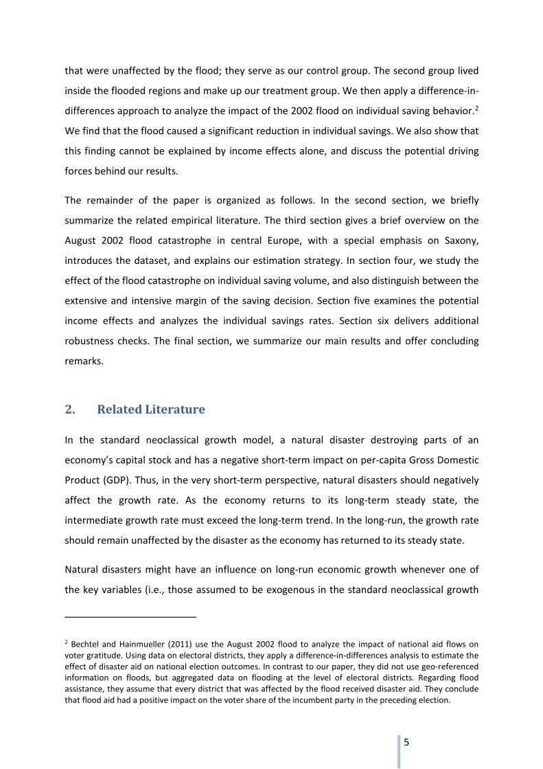
Table VIII: Saving Rate for Unrestricted Group Model Variable 2002/03 2002/04 2002/05 Tobit Dept. Var.: log SR

(I) (II) (III)

Year -0.097 (0.077) -0.092 (0.079) -0.029 (0.089)

Treated 0.0387 (0.394) 0.405 (0.394) 0.405 (0.399)

year x treated -0.102 (0.390) -1.099*(0.596) -1.097**(0.472)

Effect (in %) -9.70 -66.68 66.61

Log likelihood -3442.16 -3201.63 -3059.77


Left censored 736 685 647

The unrestricted group includes all individuals living in the treatment or control region in 2002; no further restrictions are applied. The reported coefficients show

the marginal effect on the latent variable. All listed variables are binary. Both regressions include the covariates depicted in Table I. The dependent variable SR is

censored at 0. As the interaction term is a dummy variable (D) and the dependent variable (Y) is expressed in logarithms, we compute the switch of D from 0 to 1

by 100[𝛾𝛾𝑒𝑒𝑝𝑝(𝑐𝑐𝑝𝑝𝛾𝛾𝑐𝑐𝑐𝑐𝑝𝑝𝑐𝑐𝑝𝑝𝛾𝛾𝑐𝑐𝑡𝑡) − 1]. Doing so yields the percentage change in Y when D switches from 0 to 1. As the logarithm of 0 is mathematically not defined, the

logarithm of SR is set to 0 in cases when SR is equal to 0. Moreover, as the logarithm of a number smaller than 1 is negative and saving rates are usually in between 0

and 1, the sign of the logarithm of SR was manually switched so that point estimates show the correct direction. Observations vary between regressions as the

samples are only balanced conditional on the years-to-year combination involved. We choose this procedure as to not lose additional observations. Significance

levels are reported as: * p<.10; ** p<.05; *** p<.01. Standard errors (in parentheses) are clustered on the household level.

7. Summary and Conclusions

In this paper, we presented empirical evidence illuminating the ways in which severe natural

disasters might influence individual saving behavior. Using the example of the August 2002

flood catastrophe in Europe, we showed that individual saving decisions were strongly

depressed by the flood event. While we cannot provide a formal test for this line of reasoning,

the available empirical evidence supports the hypothesis that the reduction of savings was the

consequence of the generous financial support that German policymakers provided to flood

victims in the aftermath of the catastrophe. While this policy helped to quickly overcome the

direct consequences of the disaster quite, it likely caused a Samaritan’s Dilemma by decreasing

the incentive for precautionary saving among the affected individuals. Thus, our findings

highlight the tradeoff between short-term disaster relief and long-run moral hazard effects.

Our results must be carefully interpreted, as we derived them from a natural experiment in a

highly developed country. Provided our explanation that the presence of a Samaritan’s Dilemma

30

is correct, such a dilemma can only occur as a consequence of high compensation rates. Thus,

our findings can only be transferred to situations with comparably generous disaster aid.

Our finding that natural disasters can affect individual saving behavior might also help to explain

why natural disasters tend to have long-run growth effects. Whenever saving rates permanently

decrease as a consequence of a natural disaster, this translates into lower per-capita growth.

However, in order to find out whether natural disasters do indeed have long-run consequences

for individual saving behavior, it would be necessary to track individual saving behavior for an

even longer period of time than the three year follow-up period of our empirical analysis. While

this perspective is longer than the one taken in most of the existing empirical literature, it would

be intriguing to study individual saving decisions for additional years. Due to the fact that

Saxony experienced an additional (although much less severe) flood in 2006, we refrained from

extending our econometric analysis beyond 2005. In order to shed at least some light on the

question of the long-term duration of the impact on individual saving, Figure II provides some

additional insights, which of course must be carefully interpreted.

31

Figure II shows the results when our tobit analysis is extended to the total sample period that

was available at the time when this paper was written. The analysis is based on the same

restrictions as the analysis presented in Section Four (i.e., we only consider individuals who took

part in all SOEP waves in between 2002 and 2005 and who did not move out of their home

region). We find significantly negative effects on individual saving decisions for all years until

2008. After 2008 the estimated effect is still negative and of similar size as in the preceding

years. However, the effect is rendered insignificant in these years, which is likely due to the

diminishing number of observations in the treatment group.30 While we cannot disentangle the

effect of the 2006 flood from the results of this tobit and thus should interpret these findings

very carefully, they nevertheless tend to support the view that the behavioral response to the

August 2002 flood was not a short-lived effect.

30 Figure A1 in the appendix shows that the results are similar if we use the unrestricted sample.

32

References

Aghion, P., Comin, D., Howitt, P., 2006. When Does Domestic Saving Matter for Economic Growth? NBER Working Paper No. 12275, Cambridge/Mass.

Anbarci, N., Escaleras, M., Register C.A., 2005. Earthquake fatalities: the interaction of nature and political economy. J. Public Econ. 89, 1907-1933.

Angrist, J. D., Pischke, J.-S., 2009. Mostly Harmless Econometrics. Princeton University Press, New Jersey.

Antwi-Boasiako, B.A., 2014. Why Do Few Homeowners Insure Against Natural Catastrophe Losses? forthcoming in: Rev. Econ. 65.

Bechtel, M., Hainmueller, J., 2011. How Lasting is Voter Gratitude? An Analysis of the Short- and Long-Term Electoral Returns to Beneficial Policy. Am. J. Polit. Sci. 55, 851-867.

Berlemann, M., Vogt, G., 2008. Kurzfristige Wachstumseffekte von Naturkatastrophen. Eine empirische Analyse der Flutkatastrophe vom August 2002 in Sachsen, Zeitschrift für Umweltpolitik und Umweltrecht 31, 209-232.

Berlemann, M., 2014. Hurricane Risk, Happiness and Life Satisfaction: Some Empirical Evidence on the Indirect Effects of Natural Disasters. Working Paper.

Bluedorn, J.C., 2005. Hurricanes: Intertemporal Trade and Capital Shocks. Nuffield College Economic Paper 2005-w22.

Botzen, W., Aerts, J., van den Bergh, J., 2009. Willingness of Homeowners to Mitigate Climate Risk Through Insurance. Ecol. Econ. 68, 2265–2277.

Browne, M.J., Hoyt, R.E., 2000. The Demand for Flood Insurance: Empirical Evidence. J. Risk Uncertain. 20, 291–306.

Brunette, M., Cabantous, L., Couture, S., Stenger, A., 2013. The impact of governmental assistance on insurance demand under ambiguity: a theoretical model and an experimental test. Theory and Decis. 75, 153-174.

Buchanan, J., 1975. The Samaritan’s Dilemma, in Phelps, E.S. (Ed.), Altruism, morality, and economic theory. Russell Sage Found., New York, 71–85.

Callen, M., 2011. Catastrophes and Time Preference: Evidence from the Indian Ocean Earthquake. Working Paper.

Cassar, A., Healy, A., von Kessler, C., 2011. Trust, Risk, and Time Preference after a Natural Disaster: Experimental Evidence from Thailand. University of San Francisco Working Paper.

33

https://scholar.google.com/citations?view_op=view_citation&hl=en&user=8OdhAuMAAAAJ&citation_for_view=8OdhAuMAAAAJ:fPk4N6BV_jEC



Cameron, L., Shah, M., 2013. Risk-Taking Behavior in the Wake of Natural Disasters. NBER Working Papers No. 19534.

Coate, S., 1995. Altruism, the Samaritan’s Dilemma and Government Transfer Policy. Am. Econ. Rev. 85, 46-57.

Deryugina, T., Kirwan, K., Levitt, S., 2014a. The Economic Impact of Hurricane Katrina on its Victims. Evidence from Individual Tax Returns. NBER Working Paper No. 20713.

Deryugina, T., Kirwan, B., 2014b. Does the Samaritan’s Dilemma Matter? Evidence from Corp Insurance, Working Paper.

Dobes, L., Jotzo, F., Stern, D.I., 2014. The Economics of Global Climate Change: A Historical Literature Review. forthcoming in: Rev. Econ. 65.

Dooley, M.P., Folkerts-Landau, D., Garber, P.M., 2004. The US Current Account Deficit and Economic Development: Collateral for a Total Return Swap. NBER Working Paper No. 10727, Cambridge/Mass.

Eckel, C.C., El-Gambal, M.A., Wilson, R.K., 2009. Risk Loving after the Storm: A Bayesian-Network Study of Hurricane Katrina Evacuees. J. Econ. Behav. Organ. 69, 110-124.

Felbermayr, G.J., Gröschl, J., 2014. Naturally Negative: The Growth Effects of Natural Disasters. J. Dev. Econ. 111, 92-106.

Freeman, P., Keen, M., Mani, M., 2003. Dealing with Increased Risk of Natural Disasters: Challenges and Options. IMF Working Paper WP/03/197.

Fuchs-Schündeln, N., Schündeln, M., 2005. Precautionary Savings and Self-selection: Evidence from the German Reunification “Experiment”. Q. J. Econ. 120, 1085-1120.

Groen, J.A., Polivka, A.E., 2010. Going home after Hurricane Katrina: Determinants of return migration and changes in affected areas. Demogr. 47, 821-844.

GWS - German Weather Service, 2007. Die Elbeflut im August 2002 - Fünf Jahre danach. Press Release August 2007.

Hintze, P., Lakes, T., 2009. Geographically Referenced Data in Social Science. A Service Paper for SOEP Data Users. DIW Berlin Data Documentation No. 46.

Hochrainer, S., 2009. Assessing the macroeconomic impacts of natural disasters: are there any? World Bank Policy Research Working Paper No. 4968.

Hoffmann, C. Matticzk, H., Speich, W.-D., 2004. Wirtschaftsentwicklung 2003 in Sachsen. Statistik in Sachsen 4.

Horwich, G., 2000. Economic lessons of the Kobe earthquake. Economic Development and Cultural Change 48, 521-542.

34

Hsiang, S.M. and Jina, A.S., 2014. The Causal Effects of Environmental Catastrophe on Economic Growth: Evidence from 6,700 tropical cyclones. NBER Working Paper No. 20352.

Kahn, M.E. 2005. The Death Toll from Natural Disasters: The Role of Income, Geography, and Institutions. Rev. Econ. Stat. 87, 271-284.

Kousky, C., Michel-Kerjan, E.O., Raschky, P., 2013. Does federal disaster assistance crowd out private demand for insurance? Risk Management and Decision Processes Center The Wharton School, University of Pennsylvania 2013-10.

Kunreuther, H. C., Ginsberg, R., Miller, L., Sagi, P., Slovic, P., Borkan, B., Katz, N., 1978. Disaster Insurance Protection: Public Policy Lessons. John Wiley & Sons, New York

Leitstelle Wiederaufbau, 2003a. Schadensausgleich und Wiederaufbau im Freistaat Sachsen. Staatskanzlei, Freistaat Sachsen.

Leitstelle Wiederaufbau, 2003b. Der Wiederaufbau im Freistaat Sachsen ein Jahr nach der Flut. Staatskanzlei, Freistaat Sachsen.

Linnerooth-Bayer, J., Quijano-Evans, S., Löfstedt, R, Elahi, S., 2001. The uninsured elements of natural catastrophic losses. Tsunami Project Summary Report.

Loayza, N., Olaberría, E., Rigolini, J., Christiaensen, L., 2012. Natural Disasters and Growth: Going Beyond the Averages. World Dev. 40, 1317-1336.

Löpmeier, F.-J., 2003. Die agrarmeterologische Situation, in: Klimastatusbericht 2002, Deutscher Wetterdienst, Offenbach am Main.

Luechinger, S., Raschky, P.A., 2009. Valuing flood disasters using the life satisfaction approach. J. Public Econ. 93, 620–633.

Lusardi, A., 1998. On the Importance of the Precautionary Saving Motive. Am. Econ. Rev. Pap. Proc. 88, 449–453.

Mechler, R., Weichselgartner, J., 2003. Disaster Loss Financing in Germany – The Case of the Elbe River Floods 2002. IIASA Interim Report IR-03-021.

Mechler, R., 2009. Disasters and Economic Welfare: Can National Savings Explain Post-disaster Changes in Consumption? World Bank Policy Research Working Paper No. 4988.

Müller, M., Thieken, A., 2005. Hochwasserschäden bei Unternehmen in Sachsen. Schadensprisma 2, 22-31.

Noy, I., Nualsri, A., 2007. What do exogenous shocks tell us about growth theories? Working Papers, Santa Cruz Center for International Economics 07-16.

Noy, I., 2009. The macroeconomic consequences of disasters. J. Dev. Econ. 88, 221-231.

Page, L., Savage, D., Torgler, B., 2014. Variation in risk seeking behaviour following large losses: A natural experiment. Eur. Econ. Rev. 71, 121-131.

35

http://blogs.cuit.columbia.edu/asj2122/files/2014/08/hsiang_jina_growth.pdf

http://blogs.cuit.columbia.edu/asj2122/files/2014/08/hsiang_jina_growth.pdf

http://www.nber.org/papers/w20352

Raddatz, C., 2007. Are external shocks responsible for the instability of output in low-income countries? J. Dev. Econ. 84, 155-187.

Raddatz, C., 2009. The wrath of God: macroeconomic costs of natural disasters. World Bank Policy Research Working Paper No. 5039.

Raschky, P.A., Weck-Hannemann, H., 2007. Charity Hazard - A Real Hazard to Natural Disaster Insurance? Environ. Hazards 7, 321–329.

Roson, R., Calzadilla, A., Francesco, P, 2005. Climate Change and Extreme Events: an Assessment of Economic Implications. Comp. Econ. Fin. 49, Society for Computational Economics.

Rudolf, B., Rapp. J., 2003. Das Jahrhunderthochwasser der Elbe: Synoptische Wetterentwicklung und klimatologische Aspekte, in: Klimastatusbericht 2002, Deutscher Wetterdienst, Offenbach am Main.

Sawada, Y., Shimizutani, S., 2008. How Do People Cope with Natural Disasters? Evidence from the Great Hanshin-Awaji (Kobe) Earthquake in 1995. J. Money Credit Bank. 40, 463-488.

Skidmore, M., 2001. Risk, natural disasters, and household savings in a life cycle model. Japan and the World Economy 13,15-34.

Skidmore, M., Toya, H., 2002. Do natural disasters promote long-run growth? Econ. Inq. 40, 664-687.

Strobl, E., 2012. The economic growth impact of natural disasters in developing countries: Evidence from hurricane strikes in the Central American and Caribbean regions. J. Dev. Econ. 97, 130-141.

Thomas, V., 2014. Confronting Climate-Related Disasters in Asia and the Pacific. Rev. Econ. 65, 193-207.

UNISDR – United Nations Office for Disaster Risk Reduction, 2009. Global assessment report on disaster risk reduction. United Nations, Geneva.

Van Asseldonk, M., Meuwissen, M., Huirne, R., 2002. Belief in Disaster Relief and the Demand for Public-Private Insurance Program. Appl. Econ. Perspect. Pol. 24, 196–207.

Vigdor, J., 2007. The Katrina Effect: Was There a Bright Side to the Evacuation of Greater New Orleans? B.E. J. Econ. Anal. Policy 7, 1-40.

Wagner, G.G., Frick, J.R., Schupp, J., 2007. The German Socio-Economic Panel Study (SOEP) – Scope, Evolution and Enhancements. Schmollers Jahrbuch 127, 139-169.

36

Appendix

37

Table A1: Description of Variables

Variable Description

S Amount saved per month discounted to 2000 prices using the price index provided by the German federal statistical office.

SE Binary variable. Extensive margin of the Saving decision. One if the household saves any amount per month and zero otherwise.

SI Intensive margin of saving decision. In case the household reports no savings the logarithm was set to zero.

S‘E Binary variable. One if the household saves more than EUR 50 and zero otherwise.

SR Saving rate. Amount saved divided by monthly income.

Male HHH Binary variable. One if the head of the household is male and zero if female.

Age Age of person

Homeowner Binary variable. One if household owns the dwelling they live in and zero otherwise.

Rural Binary variable. One if household lives in a rural area and otherwise.

Primary Education Reference category.

Secondary Education

Binary (factor) variable. One if the highest education obtained is secondary and zero otherwise.

Tertiary Education

Binary (factor) variable. One if the highest education obtained is tertiary and zero otherwise.

Single Reference category.

Married Binary (factor) variable. One if the person is married, zero otherwise.

Other Binary (factor) variable. One if the person is divorced, widowed or married but living apart and zero otherwise.

No child Reverence category.

One Child Binary (factor) variable. One if one child lives in household and zero otherwise.

Two Children Binary (factor) variable. One if two children live in household and zero otherwise.

Two + Children Binary (factor) variable. One if three or more children live in household and zero otherwise.

38

Table A2: Effect on Latent Saving Volume (Base Sample) Tobit Regression (1) (2) (3) Var. / Dep. Var.: S (log) S (log) S (log) Year -0.097

(0.156) -0.120 (0.160)

-0.114 (0.178)

Treated 0.145 (0.874)

0.183 (0.909)

0.154 (0.892)

Year x Treated -0.845 (0.775)

-3.944*** (1.308)

-2.301** (0.982)

Male HHH 0.214 (0.321)

0.271 (0.326)

0.259 (0.307)

Age 0.008 (0.013)

0.016 (0.013)

0.028** (0.012)

Homeowner 0.653** (0.326)

0.566* (0.327)

0.442 (0.305)

Primary 1.Secondary 0.251

(0.349) 0.282

(0.363) 0.152

(0.351) 2.Tertiary 1.392***

(0.387) 1.412*** (0.399)

1.206*** (0.381)

Working 1.Unemployed -3.678***

(0.445) -3.234*** (0.424)

-3.405*** (0.425)

2.Non-Working -0.151 (0.281)

-0.112 (0.284)

-0.285 (0.271)

Single 1.Married 0.453

(0.460) 0.247

(0.467) 0.081

(0.438) 2.Other -0.540

(0.532) -1.008* (0.547)

-1.153** (0.510)

No Child 1.One Child -0.428

(0.421) -0.720 (0.450)

0.004 (0.390)

2.Two Children -1.082** (0.507)

-0.779 (0.503)

0.021 (0.461)

3.Two + Children -2.851*** (0.994)

-2.180** (0.996)

-1.624** (0.769)

Rural -0.348 (0.403)

-0.042 (0.390)

-0.336 (0.376)

Constant 2.357*** (0.703)

2.022*** (0.703)

1.541** (0.672)

Sigma 3.600 3.654 3.604 Log pseudolikelihood -4101.809 -4094.465 -4151.829 Observations 1944 1942 1954 Censored 648 658 642 See footnotes table II. Standard errors in parentheses. Significance levels: * p < 0.10, ** p < 0.05, *** p < 0.01. SE clustered on household level.

39

Table A3: Effect on Extensive Margin (Base Sample) Probit Regression (1) (2) (3) Var. / Dep. Var.: SE SE SE Year -0.048

(0.058) -0.051 (0.059)

-0.030 (0.067)

Treated 0.120 (0.323)

0.146 (0.328)

0.125 (0.323)


-1.126*** (0.380)

-0.722** (0.302)

Male HHH 0.073 (0.111)

0.101 (0.110)

0.100 (0.105)

Age 0.003 (0.005)

0.006 (0.005)

0.010** (0.004)

Homeowner 0.117 (0.117)

0.105 (0.115)

0.044 (0.108)


(0.117) 0.059

(0.119) 0.014

(0.120) 2.Tertiary 0.362***

(0.134) 0.386*** (0.137)

0.314** (0.134)


(0.116) -0.854*** (0.114)

-0.894*** (0.115)

2.Non-Working 0.017 (0.098)

0.030 (0.097)

-0.029 (0.091)


(0.154) 0.086

(0.153) 0.039

(0.146) 2.Other -0.140

(0.177) -0.309* (0.175)

-0.355** (0.164)


(0.147) -0.227 (0.148)

-0.008 (0.131)

2.Two Children -0.294* (0.168)

-0.195 (0.171)

0.055 (0.163)

3.Two + Children -0.816*** (0.273)

-0.649** (0.274)

-0.402* (0.226)

Rural -0.104 (0.133)

0.010 (0.135)

-0.089 (0.127)

Constant 0.247 (0.232)

0.0980 (0.232)

-0.0351 (0.220)

Log pseudolikelihood -1131.638 -1137.581 -1147.591 Observations 1944 1942 1954 See footnotes table II. Standard errors in parentheses. Significance levels: * p < 0.10, ** p < 0.05, *** p < 0.01. SE clustered on household level.

40

Table A4: Effect on Intensive Margin (Base Sample) Log-Linear Regression (1) (2) (3) Var. / Dep. Var.: SI (log) SI (log) SI (log) Year -0.009

(0.041) 0.009

(0.043) -0.046 (0.049)

Treated -0.088 (0.241)

-0.033 (0.430)

-0.176 (0.320)

Year x Treated -0.512*** (0.189)

-0.362 (0.402)

-0.102 (0.268)

Male HHH -0.020 (0.089)

-0.055 (0.088)

-0.033 (0.089)

Age -0.002 (0.004)

-0.003 (0.004)

0.001 (0.004)

Homeowner 0.427*** (0.090)

0.411*** (0.086)

0.416*** (0.091)


(0.128) 0.066

(0.102) 0.167

(0.113) 2.Tertiary 0.516***

(0.141) 0.361*** (0.114)

0.499*** (0.127)


(0.135) -0.462*** (0.139)

-0.593*** (0.180)

2.Non-Working -0.257*** (0.092)

-0.169* (0.090)

-0.269*** (0.095)

Single 1.Married -0.090

(0.122) 0.033

(0.117) -0.015 (0.118)

2.Other -0.287* (0.153)

-0.125 (0.154)

-0.137 (0.154)


(0.115) -0.068 (0.124)

0.175 (0.115)

2.Two Children -0.426*** (0.158)

-0.307** (0.136)

-0.130 (0.138)

3.Two + Children -0.489* (0.273)

-0.067 (0.284)

-0.290 (0.264)

Rural -0.021 (0.111)

-0.080 (0.108)

-0.084 (0.107)

Constant 5.629*** (0.213)

5.641*** (0.206)

5.308*** (0.210)

Adjusted R2 0.165 0.134 0.166 Observations 1126 1098 1078 See footnotes table II. Standard errors in parentheses. Significance levels: * p < 0.10, ** p < 0.05, *** p < 0.01. SE clustered on household level.

41

Table A5: Effect on Saving Rate (Base Sample) Tobit Regression (1) (2) (3) Var. / Dep. Var.: SR (log) SR (log) SR (log) Year -0.070

(0.078) -0.094 (0.079)

0.003 (0.089)

Treated 0.335 (0.440)

0.361 (0.440)

0.353 (0.442)


-1.657** (0.661)

-1.064** (0.481)

Male HHH 0.130 (0.136)

0.161 (0.138)

0.165 (0.132)

Age 0.006 (0.006)

0.009 (0.006)

0.009* (0.005)

Homeowner -0.059 (0.139)

-0.077 (0.139)

-0.164 (0.131)

Primary 1.Secondary -0.089

(0.172) 0.019

(0.165) -0.071 (0.174)

2.Tertiary 0.129 (0.181)

0.273 (0.181)

0.113 (0.184)


(0.203) -1.096*** (0.194)

-1.157*** (0.207)

2.Non-Working 0.001 (0.120)

0.008 (0.118)

-0.018 (0.115)


(0.198) 0.159

(0.198) 0.168

(0.188) 2.Other -0.168

(0.236) -0.370 (0.226)

-0.398* (0.212)

No Child 1.One Child 0.082

(0.183) -0.043 (0.193)

0.025 (0.161)

2.Two Children 0.065 (0.223)

0.185 (0.225)

0.339 (0.209)

3.Two + Children -0.586 (0.418)

-0.522 (0.398)

-0.123 (0.359)

Rural -0.119 (0.168)

0.057 (0.169)

-0.042 (0.159)

Constant 0.746** (0.305)

0.558* (0.310)

0.627** (0.301)

Sigma 1.582 1.571 1.580 Log pseudolikelihood -2962.439 -2887.027 -2956.567 Observations 1,906 1,868 1,892 Censored 630 624 616 See footnotes table III. Standard errors in parentheses. Significance levels: * p < 0.10, ** p < 0.05, *** p < 0.01. SE clustered on household level.

42

Table A6: Placebo Tests (Base Sample) Model (Dep. Var.) Tobit (S) Probit (SE) Log-Linear (SI) (1) (2) (3) (4) (5) (6) Variable / Years 2000/01 2000/02 2000/01 2000/02 2000/01 2000/02 Year 0.007 (0.147) -0.281* (0.168) -0.009 (0.060) -0.104 (0.065) 0.057 (0.039) -0.011 (0.046) Treated 0.178 (0.700) 0.091 (0.699) 0.252 (0.332) 0.205 (0.317) -0.475**(0.213) -0.513**(0.200) Year x Treated -0.482 (0.750) 0.083 (0.419) -0.273 (0.315) -0.062 (0.192) 0.167 (0.164) 0.143 (0.135) Male HHH 0.386 (0.286) 0.384 (0.298) 0.113 (0.108) 0.122 (0.106) 0.162*(0.093) 0.045 (0.097) Age 0.029**(0.011) 0.019*(0.012) 0.012***(0.004) 0.007* (0.004) -0.000 (0.004) 0.001 (0.004) Homeowner 1.072***(0.282) 0.843***(0.298) 0.322***(0.113) 0.222** (0.112) 0.290*** (0.090) 0.277***(0.096) Primary 1.Secondary 0.422 (0.347) 0.258 (0.326) 0.132 (0.120) 0.063 (0.111) 0.109 (0.111) 0.135 (0.115) 2.Tertiary 1.340***(0.377) 1.136***(0.359) 0.411*** (0.137) 0.328** (0.129) 0.420***(0.126) 0.384*** (0.130) Working 1.Unemployed -2.567***(0.372) -2.464***(0.394) -0.741*** (0.107) -0.682*** (0.114) -0.455***(0.134) -0.508*** (0.131) 2.Non-Working -0.073 (0.238) -0.190 (0.249) 0.065 (0.091) -0.017 (0.091) -0.215***(0.079) -0.112 (0.092) Single 1.Married -0.005 (0.368) 0.020(0.377) 0.012 (0.136) 0.018 (0.134) -0.095 (0.124) -0.018 (0.130) 2.Other -1.029**(0.471) -0.795*(0.467) -0.410** (0.168) -0.272* (0.161) -0.058 (0.150) -0.078 (0.149) No Child

1.One Child -0.837** (0.383) -0.701*(0.394) -0.286** (0.141) -0.254*(0.142) -0.144 (0.122) -0.033 (0.129) 2.Two Children -0.868** (0.436) -0.825*(0.429) -0.283* (0.158) -0.255*(0.153) -0.243 (0.156) -0.159 (0.161) 3.Two + Children -1.498** (0.741) -1.429*(0.772) -0.486* (0.256) -0.454*(0.259) -0.420 (0.275) -0.206 (0.273) Rural -0.522 (0.345) -0.463 (0.354) -0.142 (0.128) -0.120 (0.127) -0.136 (0.106) -0.244**(0.118) Constant 1.533** (0.598) 2.175***(0.612) -0.107 (0.209) 0.184 (0.215) 5.416***(0.198) 5.319***(0.205) Sigma 3.363 3.455 NA NA NA NA Log pseudolikelihood -4723.563 -4433.054 -1239.318 -1207.232 NA NA Adjusted. R2 NA NA NA NA 0.097 0.079 Observations 2220 2074 2220 2074 1338 1204 Censored 677 646 NA NA NA NA See footnotes table IV. Significance levels: * p < 0.10, ** p < 0.05, *** p < 0.01. SE clustered on household level.

43

Table A7: Placebo Test – Saving Rate (Base Sample) Tobit Regression (1) (2) Var. / Dep. Var.: SR (log) SR (log) Year -0.047

(0.077) -0.078 (0.089)

Treated 0.580 (0.426)

0.544 (0.424)


-0.266 (0.279)

Male HHH 0.015 (0.132)

0.071 (0.139)

Age 0.009 (0.005)

0.006 (0.006)

Homeowner 0.177 (0.128)

0.086 (0.138)


(0.165) -0.001 (0.165)

2.Tertiary 0.251 (0.176)

0.155 (0.180)


(0.174) -0.795*** (0.210)

2.Non-Working 0.053 (0.107)

-0.049 (0.122)


(0.169) 0.162

(0.180) 2.Other -0.403*

(0.212) -0.276 (0.215)


(0.173) -0.153 (0.192)

2.Two Children -0.021 (0.205)

-0.015 (0.211)

3.Two + Children -0.052 (0.375)

-0.120 (0.400)

Rural -0.133 (0.160)

-0.088 (0.176)

Constant 0.602** (0.272)

0.905***

(0.296) Sigma 1.549 1.631 Log pseudolikelihood -3385.833 -3224.109 Observations 2146 2004 Censored 650 622 See footnotes table V. Standard errors in parentheses. Significance levels: * p < 0.10, ** p < 0.05, *** p < 0.01. SE clustered on household level.

44

Table A8: Stability Test – Effect on Extensive Margin (Base Sample) Log-Linear Regression (1) (2) (3) Var. / Dep. Var.: S’E [S’E=1|S > 50€] S’E (log) S’E (log) S’E (log) Year 0.008

(0.059) 0.019

(0.056) -0.038 (0.066)

Treated 0.252 (0.320)

0.275 (0.325)

0.278 (0.320)


-1.207***

(0.380) -0.747** (0.304)

Male HHH 0.085 (0.109)

0.116 (0.110)

0.106 (0.103)

Age 0.005 (0.005)

0.007 (0.005)

0.012*** (0.004)

Homeowner 0.169 (0.114)

0.128 (0.114)

0.078 (0.107)


(0.114) 0.159

(0.121) 0.130

(0.119) 2.Tertiary 0.570***

(0.132) 0.543*** (0.141)

0.487*** (0.134)


(0.119) -0.868*** (0.114)

-0.961*** (0.113)

2.Non-Working -0.018 (0.097)

0.012 (0.097)

-0.045 (0.092)


(0.154) 0.050

(0.153) -0.065 (0.146)

2.Other -0.273 (0.177)

-0.378** (0.178)

-0.470*** (0.166)


(0.147) -0.156 (0.148)

0.060 (0.134)

2.Two Children -0.244 (0.168)

-0.124 (0.170)

0.135 (0.159)

3.Two + Children -0.795*** (0.277)

-0.598** (0.275)

-0.442* (0.238)

Rural -0.093 (0.132)

0.010 (0.133)

-0.063 (0.126)

Constant -0.095 (0.235)

-0.189 (0.237)

-0.355 (0.220)

Log pseudolikelihood -1158.935 -1167.622 -1182.126 Observations 1,944 1,942 1,954 See footnotes table VI. Standard errors in parentheses. Significance levels: * p < 0.10, ** p < 0.05, *** p < 0.01. SE clustered on household level.

45

Table A9: Stability Test – Saving Volume (Unrestricted Sample) Tobit Regression (1) (2) (3) Var. / Dep. Var.: S (log) S (log) S (log) Year -0.178

(0.151) -0.145 (0.158)

-0.164 (0.178)

Treated 0.215 (0.787)

0.181 (0.812)

0.430 (0.817)


-3.139*** (1.169)

-2.305** (0.934)

Male HHH 0.368 (0.313)

0.168 (0.311)

0.365 (0.307)

Age 0.014 (0.013)

0.017 (0.013)

0.033*** (0.012)

Homeowner 0.779** (0.315)

0.587* (0.312)

0.409 (0.305)


(0.315) 0.230

(0.332) 0.135

(0.337) 2.Tertiary 1.313***

(0.363) 1.368*** (0.371)

1.158*** (0.372)


(0.411) -2.952*** (0.405)

-3.526*** (0.417)

2.Non-Working -0.198 (0.270)

-0.204 (0.269)

-0.415 (0.270)


(0.430) 0.124

(0.441) -0.141 (0.428)

2.Other -0.666 (0.498)

-1.174** (0.525)

-1.345*** (0.500)


(0.409) -0.748* (0.425)

-0.067 (0.389)

2.Two Children -1.117** (0.496)

-0.681 (0.478)

0.019 (0.456)

3.Two + Children -2.346*** (0.894)

-1.968** (0.922)

-1.553** (0.751)

Rural -0.409 (0.392)

-0.074 (0.381)

-0.319 (0.375)

Constant 2.161*** (0.652)

2.161*** (0.647)

1.477** (0.650)

Sigma 3.644 3.657 3.639 Log pseudolikelihood -4705.083 -4485.792 -4299.551 Observations 2228 2122 2028 Censored 752 717 676 See footnotes table VII. Standard errors in parentheses. Significance levels: * p < 0.10, ** p < 0.05, *** p < 0.01. SE clustered on household level.

46

Table A10: Stability Test – Extensive Margin (Unrestricted Sample) Probit Regression (1) (2) (3) Var. / Dep. Var.: SE SE SE Year -0.072

(0.055) -0.053 (0.058)

-0.049 (0.066)

Treated 0.140 (0.299)

0.143 (0.302)

0.210 (0.304)


-0.871** (0.363)

-0.704** (0.301)

Male HHH 0.120 (0.105)

0.062 (0.105)

0.138 (0.103)

Age 0.005 (0.004)

0.006 (0.004)

0.012*** (0.004)

Homeowner 0.163 (0.111)

0.113 (0.109)

0.029 (0.106)


(0.104) 0.037

(0.109) 0.010

(0.115) 2.Tertiary 0.324***

(0.125) 0.365*** (0.128)

0.295** (0.130)


(0.108) -0.787*** (0.110)

-0.931*** (0.111)

2.Non-Working -0.008 (0.092)

-0.003 (0.091)

-0.072 (0.089)


(0.142) 0.035

(0.146) -0.054 (0.143)

2.Other -0.181 (0.164)

-0.365** (0.169)

-0.438*** (0.161)


(0.141) -0.234* (0.140)

-0.022 (0.130)

2.Two Children -0.311* (0.160)

-0.163 (0.163)

0.052 (0.158)

3.Two + Children -0.671*** (0.256)

-0.604** (0.256)

-0.367* (0.221)

Rural -0.120 (0.127)

-0.005 (0.130)

-0.085 (0.125)

Constant 0.216 (0.215)

0.186 (0.216)

-0.046 (0.212)

Log pseudolikelihood -1320.215 -1258.447 -1196.082 Observations 2228 2122 2028 See footnotes table VII. Standard errors in parentheses. Significance levels: * p < 0.10, ** p < 0.05, *** p < 0.01. SE clustered on household level.

47

Table A11: Stability Test - Intensive Margin (Unrestricted Sample) Log-Linear Regression (1) (2) (3) Var. / Dep. Var.: SI (log) SI (log) SI (log) Year -0.006

(0.038) 0.005

(0.042) -0.047 (0.049)

Treated -0.207 (0.207)

-0.305 (0.313)

-0.130 (0.292)


-0.512 (0.375)

-0.236 (0.280)

Male HHH -0.009 (0.087)

-0.064 (0.085)

-0.052 (0.088)

Age -0.001 (0.004)

-0.002 (0.004)

-0.000 (0.004)

Homeowner 0.409*** (0.086)

0.409*** (0.086)

0.415*** (0.091)


(0.113) 0.111

(0.096) 0.173

(0.113) 2.Tertiary 0.555***

(0.130) 0.394*** (0.109)

0.506*** (0.126)


(0.119) -0.440*** (0.130)

-0.540*** (0.176)

2.Non-Working -0.220** (0.088)

-0.173* (0.088)

-0.265*** (0.095)

Single 1.Married -0.049

(0.126) 0.142

(0.110) 0.071

(0.114) 2.Other -0.245

(0.151) -0.043 (0.146)

-0.037 (0.152)


(0.113) -0.059 (0.120)

0.149 (0.113)

2.Two Children -0.361** (0.166)

-0.285** (0.130)

-0.144 (0.137)

3.Two + Children -0.438* (0.239)

0.018 (0.246)

-0.348 (0.256)

Rural -0.038 (0.105)

-0.081 (0.102)

-0.073 (0.106)

Constant 5.471*** (0.198)

5.464*** (0.196)

5.345*** (0.206)

Adjusted R2 0.156 0.145 0.164 Observations 1278 1198 1104 See footnotes table VII. Standard errors in parentheses. Significance levels: * p < 0.10, ** p < 0.05, *** p < 0.01. SE clustered on household level.

48

Table A12: Effect on Saving Rate (Unrestricted Sample) Tobit Regression (1) (2) (3) Var. / Dep. Var.: SR (log) SR (log) SR (log) Year -0.097

(0.077) -0.092 (0.079)

-0.029 (0.089)

Treated 0.387 (0.394)

0.405 (0.394)

0.457 (0.399)


-1.097* (0.596)

-1.038** (0.472)

Male HHH 0.204 (0.138)

0.123 (0.136)

0.213 (0.131)

Age 0.009 (0.006)

0.010* (0.006)

0.012** (0.005)

Homeowner 0.023 (0.140)

-0.064 (0.137)

-0.190 (0.130)

Primary 1.Secondary -0.047

(0.158) -0.031 (0.155)

-0.084 (0.168)

2.Tertiary 0.127 (0.174)

0.238 (0.170)

0.090 (0.180)


(0.190) -1.009*** (0.190)

-1.233*** (0.203)

2.Non-Working -0.072 (0.117)

-0.023 (0.115)

-0.075 (0.115)


(0.195) 0.011

(0.199) 0.004

(0.186) 2.Other -0.291

(0.224) -0.551** (0.229)

-0.569*** (0.210)

No Child 1.One Child 0.096

(0.182) -0.020 (0.188)

0.044 (0.159)

2.Two Children 0.052 (0.225)

0.253 (0.220)

0.334 (0.204)

3.Two + Children -0.353 (0.428)

-0.431 (0.402)

-0.058 (0.357)

Rural -0.103 (0.173)

0.087 (0.171)

-0.043 (0.157)

Constant 0.687** (0.293)

0.669** (0.297)

0.620** (0.292)

Sigma 1.639 1.615 1.592 Log pseudolikelihood -3442.161 -3201.631 -3059.770 Observations 2,188 2,044 1,960 Censored 736 685 647 See footnotes table VIII. Standard errors in parentheses. Significance levels: * p < 0.10, ** p < 0.05, *** p < 0.01. SE clustered on household level.

49

Date post:	10-May-2020
Category:	Documents
Upload:	others
View:	2 times
Download:	0 times

Do Natural Disasters Stimulate Individual Saving? Evidence ...ftp.iza.org/dp9026.pdf · developed...

Documents