Do the RIM (Residual Income Model), EVA ® and DCF (Discounted Cash Flow) Really Match? Ignacio Vélez-Pareja Politécnico Grancolombiano Bogotá, Colombia [email protected]Joseph Tham Boston University [email protected]Working Paper N 25 First version: 2003-01-12 This version: 2003-06-27
Transcript
Do the RIM (Residual Income Model), EVA® and DCF (Discounted Cash Flow)
Working Paper N 25 First version: 2003-01-12 This version: 2003-06-27
2
Abstract In Vélez-Pareja and Tham (2001), we presented several different ways to value
cash flows. First, we apply the standard after-tax Weighted Average Cost of Capital, WACC to the free cash flow (FCF). Second, we apply the adjusted WACC to the FCF, and third we apply the WACC to the capital cash flow. In addition, we discount the cash flow to equity (CFE) with the appropriate returns to levered equity. We refer to these four ways as the “discounted cash flow (DCF)” methods.
In recent years, two new approaches, the Residual Income Method (RIM) and the Economic Value Added (EVA) have become very popular. Supporters claim the RIM and EVA are superior to the DCF methods. It may be case that the RIM and EVA approaches are useful tools for assessing managerial performance and providing proper incentives. However, from a valuation point of view, the RIM and EVA are problematic because they use book values from the balance sheet. It is easy to show that under certain conditions, the results from the RIM and EVA exactly match the results from the DCF methods.
Velez-Pareja 1999 reported that when using relatively complex examples and book values to calculate Economic Value Added (EVA), the results were inconsistent with Net Present Value (NPV). Tham 2001, reported consistency between the Residual Income Model (RIM) and the Discounted Cash Flow model (DCF) with a very simple example. Fernandez 2002 shows examples where there is consistency between DCF, RIM and EVA. He uses a constant value for the cost of levered equity capital and in another example constant debt. Young and O’Byrne, 2001, show simple examples for EVA but do not show the equivalence between DCF and EVA. Ehrbar (1998) uses a very simple example with perpetuities and shows the equivalence between EVA and DCF. Lundholm and O'Keefe, 2001, show this equivalence with an example with constant Ke. Tham 2001, commented on their paper. Stewart, 1999, shows the equivalence between DCF and EVA with an example using a constant discount rate. Copeland, et al, show an example with constant WACC and constant cost of equity even with varying debt and assuming a target leverage that is different to the actual leverage.
In general, textbooks do not specify clearly how EVA should be used to give consistent results.
In this teaching note using a complex example with varying debt, varying leverage and terminal (or continuing value), we show the consistency between DCF, RIM and EVA. We stress what Velez-Pareja 1999 and Fernandez 2002 said: for a single period, RI or EVA does not measure value. We have to include expectations and market values in the calculation of discount rates and hence values.
Keywords Economic Value Added, EVA, Market Value Added, MVA, Net Present Value,
NPV, cash flows, free cash flows, market value of equity, market value of the firm.
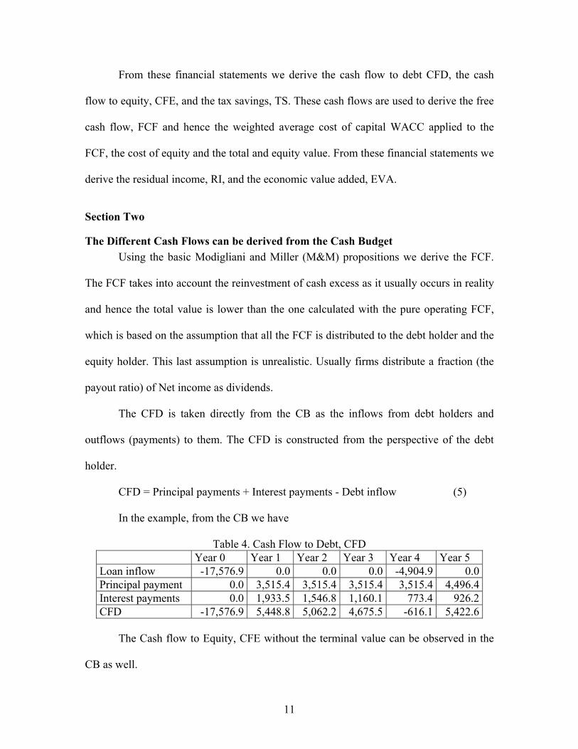
Table 4. Cash Flow to Debt, CFD Year 0 Year 1 Year 2 Year 3 Year 4 Year 5 Loan inflow -17,576.9 0.0 0.0 0.0 -4,904.9 0.0Principal payment 0.0 3,515.4 3,515.4 3,515.4 3,515.4 4,496.4Interest payments 0.0 1,933.5 1,546.8 1,160.1 773.4 926.2CFD -17,576.9 5,448.8 5,062.2 4,675.5 -616.1 5,422.6
The Cash flow to Equity, CFE without the terminal value can be observed in the
CB as well.
12
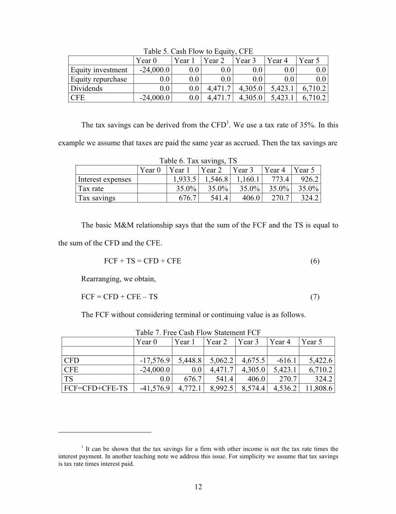
Table 5. Cash Flow to Equity, CFE Year 0 Year 1 Year 2 Year 3 Year 4 Year 5 Equity investment -24,000.0 0.0 0.0 0.0 0.0 0.0Equity repurchase 0.0 0.0 0.0 0.0 0.0 0.0Dividends 0.0 0.0 4,471.7 4,305.0 5,423.1 6,710.2CFE -24,000.0 0.0 4,471.7 4,305.0 5,423.1 6,710.2
The tax savings can be derived from the CFD1. We use a tax rate of 35%. In this
example we assume that taxes are paid the same year as accrued. Then the tax savings are
Table 6. Tax savings, TS Year 0 Year 1 Year 2 Year 3 Year 4 Year 5 Interest expenses 1,933.5 1,546.8 1,160.1 773.4 926.2Tax rate 35.0% 35.0% 35.0% 35.0% 35.0%Tax savings 676.7 541.4 406.0 270.7 324.2
The basic M&M relationship says that the sum of the FCF and the TS is equal to
the sum of the CFD and the CFE.
FCF + TS = CFD + CFE (6)
Rearranging, we obtain,
FCF = CFD + CFE – TS (7)
The FCF without considering terminal or continuing value is as follows.
Table 7. Free Cash Flow Statement FCF Year 0 Year 1 Year 2 Year 3 Year 4 Year 5 CFD -17,576.9 5,448.8 5,062.2 4,675.5 -616.1 5,422.6CFE -24,000.0 0.0 4,471.7 4,305.0 5,423.1 6,710.2TS 0.0 676.7 541.4 406.0 270.7 324.2FCF=CFD+CFE-TS -41,576.9 4,772.1 8,992.5 8,574.4 4,536.2 11,808.6
1 It can be shown that the tax savings for a firm with other income is not the tax rate times the interest payment. In another teaching note we address this issue. For simplicity we assume that tax savings is tax rate times interest paid.
13
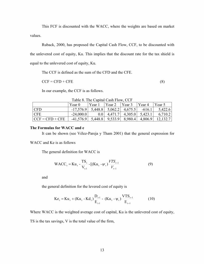
This FCF is discounted with the WACC, where the weights are based on market
values.
Ruback, 2000, has proposed the Capital Cash Flow, CCF, to be discounted with
the unlevered cost of equity, Ku. This implies that the discount rate for the tax shield is
equal to the unlevered cost of equity, Ku.
The CCF is defined as the sum of the CFD and the CFE.
CCF = CFD + CFE (8)
In our example, the CCF is as follows.
Table 8. The Capital Cash Flow, CCF Year 0 Year 1 Year 2 Year 3 Year 4 Year 5 CFD -17,576.9 5,448.8 5,062.2 4,675.5 -616.1 5,422.6CFE -24,000.0 0.0 4,471.7 4,305.0 5,423.1 6,710.2CCF = CFD + CFE -41,576.9 5,448.8 9,533.9 8,980.4 4,806.9 12,132.7
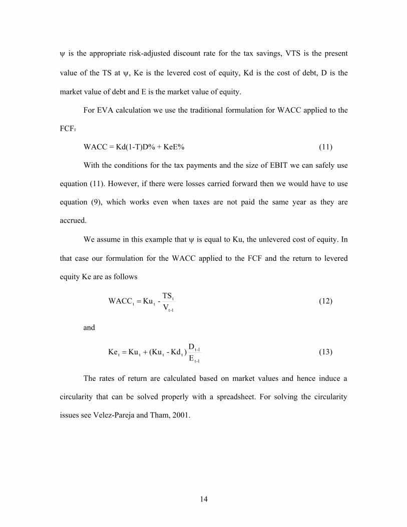
The Formulas for WACC and e It can be shown (see Vélez-Pareja y Tham 2001) that the general expression for
WACC and Ke is as follows
The general definition for WACC is
1
1t
1-t
ttt ) - [(Ku -
VTS
- Ku WACC−
−=t
tt V
VTSψ (9)
and
the general definition for the levered cost of equity is
1t
1ttt
1-t
1-ttttt E
VTS)ψ - (Ku -
ED
)Kd - (Ku Ku Ke−
−+= (10)
Where WACC is the weighted average cost of capital, Ku is the unlevered cost of equity,
TS is the tax savings, V is the total value of the firm,
14
ψ is the appropriate risk-adjusted discount rate for the tax savings, VTS is the present
value of the TS at ψ, Ke is the levered cost of equity, Kd is the cost of debt, D is the
market value of debt and E is the market value of equity.
For EVA calculation we use the traditional formulation for WACC applied to the
FCF.
WACC = Kd(1-T)D% + KeE% (11)
With the conditions for the tax payments and the size of EBIT we can safely use
equation (11). However, if there were losses carried forward then we would have to use
equation (9), which works even when taxes are not paid the same year as they are
accrued.
We assume in this example that ψ is equal to Ku, the unlevered cost of equity. In
that case our formulation for the WACC applied to the FCF and the return to levered
equity Ke are as follows
1-t
ttt V
TS - Ku WACC = (12)
and
1-t
1-ttttt E
D)Kd - (Ku Ku Ke += (13)
The rates of return are calculated based on market values and hence induce a
circularity that can be solved properly with a spreadsheet. For solving the circularity
issues see Velez-Pareja and Tham, 2001.
15
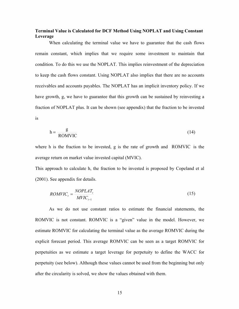
Terminal Value is Calculated for DCF Method Using NOPLAT and Using Constant Leverage
When calculating the terminal value we have to guarantee that the cash flows
remain constant, which implies that we require some investment to maintain that
condition. To do this we use the NOPLAT. This implies reinvestment of the depreciation
to keep the cash flows constant. Using NOPLAT also implies that there are no accounts
receivables and accounts payables. The NOPLAT has an implicit inventory policy. If we
have growth, g, we have to guarantee that this growth can be sustained by reinvesting a
fraction of NOPLAT plus. It can be shown (see appendix) that the fraction to be invested
is
ROMVIC g h = (14)
where h is the fraction to be invested, g is the rate of growth and ROMVIC is the
average return on market value invested capital (MVIC).
This approach to calculate h, the fraction to be invested is proposed by Copeland et al
(2001). See appendix for details.
1−
=t
tt MVIC
NOPLATROMVIC (15)
As we do not use constant ratios to estimate the financial statements, the
ROMVIC is not constant. ROMVIC is a “given” value in the model. However, we
estimate ROMVIC for calculating the terminal value as the average ROMVIC during the
explicit forecast period. This average ROMVIC can be seen as a target ROMVIC for
perpetuities as we estimate a target leverage for perpetuity to define the WACC for
perpetuity (see below). Although these values cannot be used from the beginning but only
after the circularity is solved, we show the values obtained with them.
16
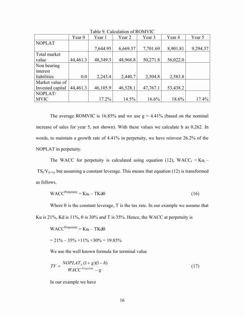
Table 9. Calculation of ROMVIC Year 0 Year 1 Year 2 Year 3 Year 4 Year 5 NOPLAT
7,644.95 6,669.57 7,701.69
8,901.81
9,294.37 Total market value 44,461.3 48,349.3 48,968.8 50,271.8 56,022.0 Non bearing interest liabilities 0.0 2,243.4 2,440.7 2,504.8 2,583.8 Market value of Invested capital 44,461.3 46,105.9 46,528.1 47,767.1 53,438.2 NOPLAT/ MVIC 17.2% 14.5% 16.6% 18.6% 17.4%
The average ROMVIC is 16.85% and we use g = 4.41% (based on the nominal
increase of sales for year 5, not shown). With these values we calculate h as 0.262. In
words, to maintain a growth rate of 4.41% in perpetuity, we have reinvest 26.2% of the
NOPLAT in perpetuity.
The WACC for perpetuity is calculated using equation (12), WACCt = Kut –
TSt/V(t-1), but assuming a constant leverage. This means that equation (12) is transformed
as follows.
WACCPerpetuity = Kut – TKdθ (16)
Where θ is the constant leverage, T is the tax rate. In our example we assume that
Ku is 21%, Kd is 11%, θ is 30% and T is 35%. Hence, the WACC at perpetuity is
WACCPerpetuity = Kut – TKdθ
= 21% – 35% ×11% ×30% = 19.85%
We use the well known formula for terminal value
gWACChgNOPLAT
TV PerpetuityN
−−+
=)1)(1(
(17)
In our example we have
17
%41.4%85.19)262.01)(0441.01(4.294,9
−−+
=TV
= 46,415.3
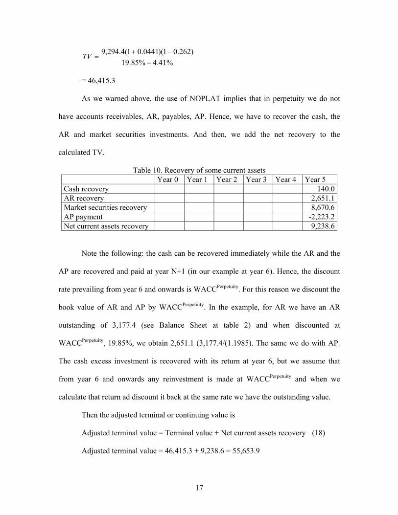
As we warned above, the use of NOPLAT implies that in perpetuity we do not
have accounts receivables, AR, payables, AP. Hence, we have to recover the cash, the
AR and market securities investments. And then, we add the net recovery to the
calculated TV.
Table 10. Recovery of some current assets Year 0 Year 1 Year 2 Year 3 Year 4 Year 5 Cash recovery 140.0AR recovery 2,651.1Market securities recovery 8,670.6AP payment -2,223.2Net current assets recovery 9,238.6
Note the following: the cash can be recovered immediately while the AR and the
AP are recovered and paid at year N+1 (in our example at year 6). Hence, the discount
rate prevailing from year 6 and onwards is WACCPerpetuity. For this reason we discount the
book value of AR and AP by WACCPerpetuity. In the example, for AR we have an AR
outstanding of 3,177.4 (see Balance Sheet at table 2) and when discounted at
WACCPerpetuity, 19.85%, we obtain 2,651.1 (3,177.4/(1.1985). The same we do with AP.
The cash excess investment is recovered with its return at year 6, but we assume that
from year 6 and onwards any reinvestment is made at WACCPerpetuity and when we
calculate that return ad discount it back at the same rate we have the outstanding value.
Then the adjusted terminal or continuing value is
Adjusted terminal value = Terminal value + Net current assets recovery (18)
Adjusted terminal value = 46,415.3 + 9,238.6 = 55,653.9
18
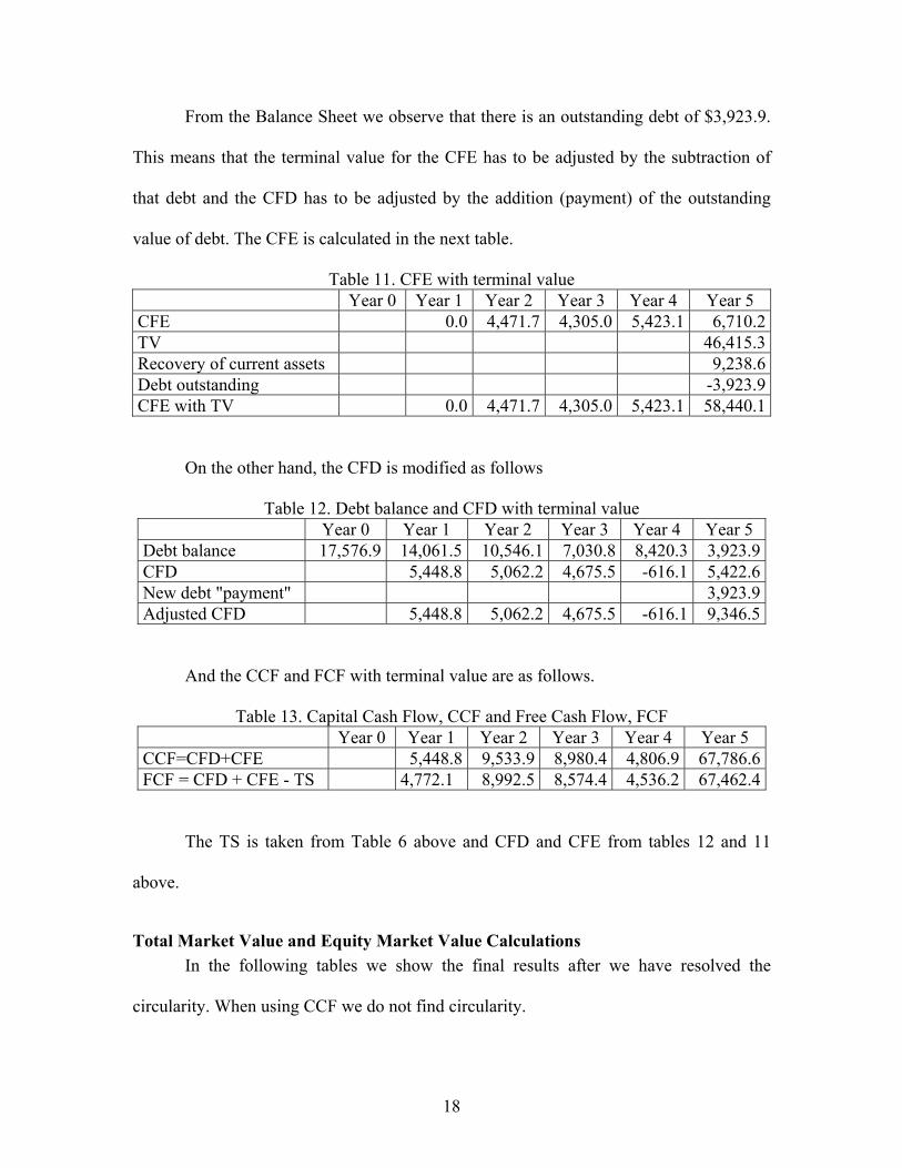
From the Balance Sheet we observe that there is an outstanding debt of $3,923.9.
This means that the terminal value for the CFE has to be adjusted by the subtraction of
that debt and the CFD has to be adjusted by the addition (payment) of the outstanding
value of debt. The CFE is calculated in the next table.
Table 11. CFE with terminal value Year 0 Year 1 Year 2 Year 3 Year 4 Year 5 CFE 0.0 4,471.7 4,305.0 5,423.1 6,710.2TV 46,415.3Recovery of current assets 9,238.6Debt outstanding -3,923.9CFE with TV 0.0 4,471.7 4,305.0 5,423.1 58,440.1
On the other hand, the CFD is modified as follows
Table 12. Debt balance and CFD with terminal value Year 0 Year 1 Year 2 Year 3 Year 4 Year 5 Debt balance 17,576.9 14,061.5 10,546.1 7,030.8 8,420.3 3,923.9CFD 5,448.8 5,062.2 4,675.5 -616.1 5,422.6New debt "payment" 3,923.9Adjusted CFD 5,448.8 5,062.2 4,675.5 -616.1 9,346.5
And the CCF and FCF with terminal value are as follows.
Table 13. Capital Cash Flow, CCF and Free Cash Flow, FCF Year 0 Year 1 Year 2 Year 3 Year 4 Year 5 CCF=CFD+CFE 5,448.8 9,533.9 8,980.4 4,806.9 67,786.6FCF = CFD + CFE - TS 4,772.1 8,992.5 8,574.4 4,536.2 67,462.4
The TS is taken from Table 6 above and CFD and CFE from tables 12 and 11
above.
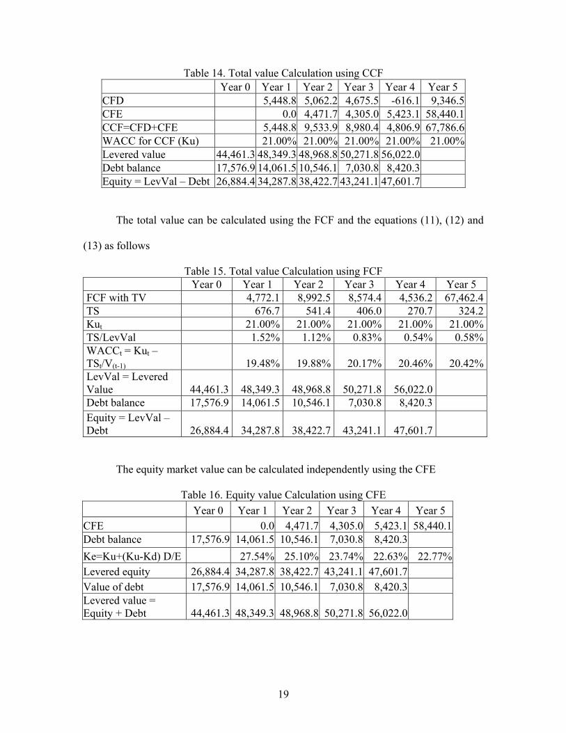
Total Market Value and Equity Market Value Calculations In the following tables we show the final results after we have resolved the
circularity. When using CCF we do not find circularity.
19
Table 14. Total value Calculation using CCF Year 0 Year 1 Year 2 Year 3 Year 4 Year 5 CFD 5,448.8 5,062.2 4,675.5 -616.1 9,346.5CFE 0.0 4,471.7 4,305.0 5,423.1 58,440.1CCF=CFD+CFE 5,448.8 9,533.9 8,980.4 4,806.9 67,786.6WACC for CCF (Ku) 21.00% 21.00% 21.00% 21.00% 21.00%Levered value 44,461.3 48,349.3 48,968.8 50,271.8 56,022.0 Debt balance 17,576.9 14,061.5 10,546.1 7,030.8 8,420.3 Equity = LevVal – Debt 26,884.4 34,287.8 38,422.7 43,241.1 47,601.7
The total value can be calculated using the FCF and the equations (11), (12) and
(13) as follows
Table 15. Total value Calculation using FCF Year 0 Year 1 Year 2 Year 3 Year 4 Year 5 FCF with TV 4,772.1 8,992.5 8,574.4 4,536.2 67,462.4TS 676.7 541.4 406.0 270.7 324.2Kut 21.00% 21.00% 21.00% 21.00% 21.00%TS/LevVal 1.52% 1.12% 0.83% 0.54% 0.58%WACCt = Kut – TSt/V(t-1) 19.48% 19.88% 20.17% 20.46% 20.42%LevVal = Levered Value 44,461.3 48,349.3 48,968.8 50,271.8 56,022.0 Debt balance 17,576.9 14,061.5 10,546.1 7,030.8 8,420.3 Equity = LevVal – Debt 26,884.4 34,287.8 38,422.7 43,241.1 47,601.7
The equity market value can be calculated independently using the CFE
Table 16. Equity value Calculation using CFE Year 0 Year 1 Year 2 Year 3 Year 4 Year 5 CFE 0.0 4,471.7 4,305.0 5,423.1 58,440.1 Debt balance 17,576.9 14,061.5 10,546.1 7,030.8 8,420.3 Ke=Ku+(Ku-Kd) D/E 27.54% 25.10% 23.74% 22.63% 22.77% Levered equity 26,884.4 34,287.8 38,422.7 43,241.1 47,601.7 Value of debt 17,576.9 14,061.5 10,546.1 7,030.8 8,420.3 Levered value = Equity + Debt 44,461.3 48,349.3 48,968.8 50,271.8 56,022.0
20
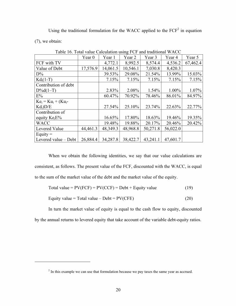
Using the traditional formulation for the WACC applied to the FCF2 in equation
(7), we obtain:
Table 16. Total value Calculation using FCF and traditional WACC Year 0 Year 1 Year 2 Year 3 Year 4 Year 5 FCF with TV 4,772.1 8,992.5 8,574.4 4,536.2 67,462.4Value of Debt 17,576.9 14,061.5 10,546.1 7,030.8 8,420.3 D% 39.53% 29.08% 21.54% 13.99% 15.03%Kdi(1-T) 7.15% 7.15% 7.15% 7.15% 7.15%Contribution of debt D%d(1–T) 2.83% 2.08% 1.54% 1.00% 1.07%E% 60.47% 70.92% 78.46% 86.01% 84.97%Kei = Kui + (Kui-Kdi)D/E 27.54% 25.10% 23.74% 22.63% 22.77%Contribution of equity KeiE% 16.65% 17.80% 18.63% 19.46% 19.35%WACC 19.48% 19.88% 20.17% 20.46% 20.42%Levered Value 44,461.3 48,349.3 48,968.8 50,271.8 56,022.0 Equity = Levered value – Debt 26,884.4 34,287.8 38,422.7 43,241.1 47,601.7
When we obtain the following identities, we say that our value calculations are
consistent, as follows. The present value of the FCF, discounted with the WACC, is equal
to the sum of the market value of the debt and the market value of the equity.
Total value = PV(FCF) = PV(CCF) = Debt + Equity value (19)
Equity value = Total value – Debt = PV(CFE) (20)
In turn the market value of equity is equal to the cash flow to equity, discounted
by the annual returns to levered equity that take account of the variable debt-equity ratios.
2 In this example we can use that formulation because we pay taxes the same year as accrued.
21
Section Three
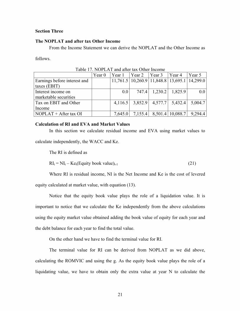
The NOPLAT and after tax Other Income From the Income Statement we can derive the NOPLAT and the Other Income as
follows.
Table 17. NOPLAT and after tax Other Income Year 0 Year 1 Year 2 Year 3 Year 4 Year 5 Earnings before interest and taxes (EBIT)
11,761.5 10,260.9 11,848.8 13,695.1 14,299.0
Interest income on marketable securities
0.0 747.4 1,230.2 1,825.9 0.0
Tax on EBIT and Other Income
4,116.5 3,852.9 4,577.7 5,432.4 5,004.7
NOPLAT + After tax OI 7,645.0 7,155.4 8,501.4 10,088.7 9,294.4
Calculation of RI and EVA and Market Values In this section we calculate residual income and EVA using market values to
calculate independently, the WACC and Ke.
The RI is defined as
RIt = NIt – Ket(Equity book value)t-1 (21)
Where RI is residual income, NI is the Net Income and Ke is the cost of levered
equity calculated at market value, with equation (13).
Notice that the equity book value plays the role of a liquidation value. It is
important to notice that we calculate the Ke independently from the above calculations
using the equity market value obtained adding the book value of equity for each year and
the debt balance for each year to find the total value.
On the other hand we have to find the terminal value for RI.
The terminal value for RI can be derived from NOPLAT as we did above,
calculating the ROMVIC and using the g. As the equity book value plays the role of a
liquidating value, we have to obtain only the extra value at year N to calculate the
22
terminal value for RI. As we did above, we have to recover some current assets and “pay”
the debt outstanding.
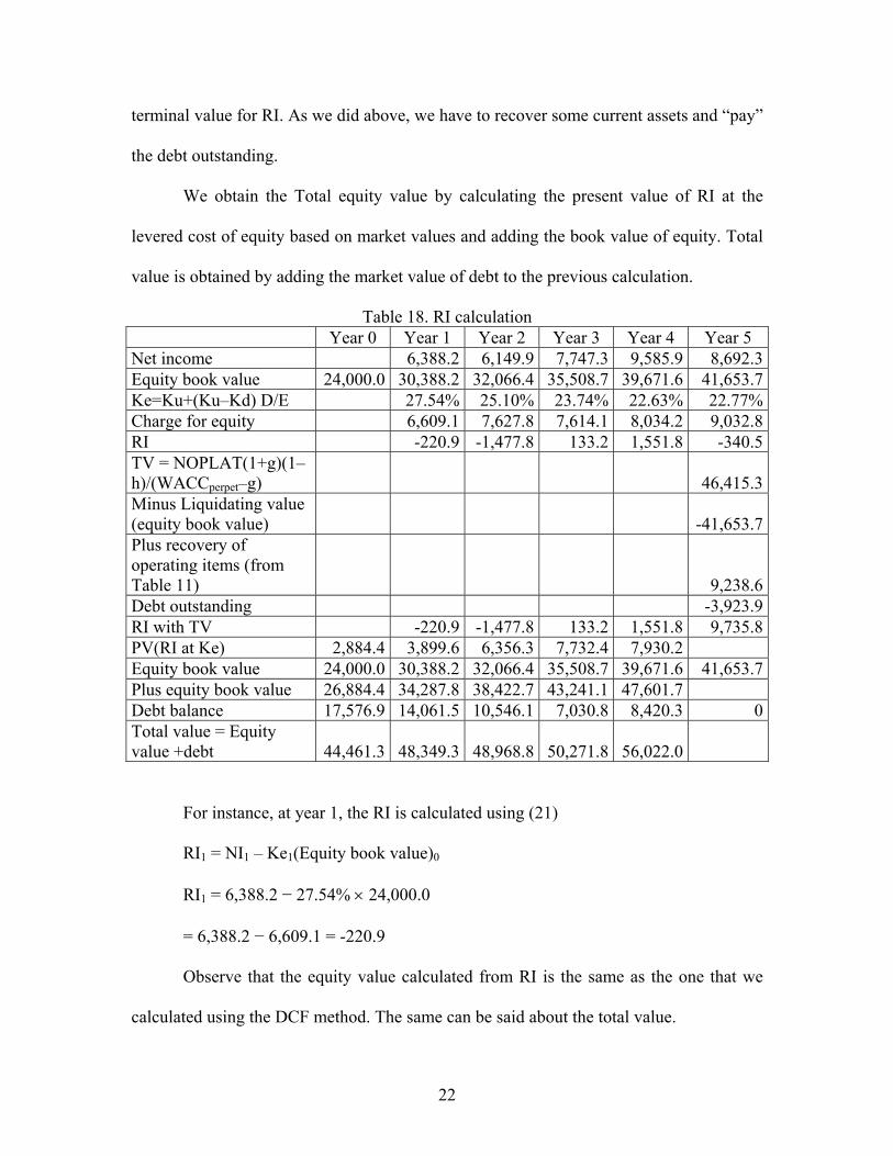
We obtain the Total equity value by calculating the present value of RI at the
levered cost of equity based on market values and adding the book value of equity. Total
value is obtained by adding the market value of debt to the previous calculation.
Table 18. RI calculation Year 0 Year 1 Year 2 Year 3 Year 4 Year 5 Net income 6,388.2 6,149.9 7,747.3 9,585.9 8,692.3Equity book value 24,000.0 30,388.2 32,066.4 35,508.7 39,671.6 41,653.7Ke=Ku+(Ku–Kd) D/E 27.54% 25.10% 23.74% 22.63% 22.77%Charge for equity 6,609.1 7,627.8 7,614.1 8,034.2 9,032.8RI -220.9 -1,477.8 133.2 1,551.8 -340.5TV = NOPLAT(1+g)(1–h)/(WACCperpet–g)
46,415.3
Minus Liquidating value (equity book value)
-41,653.7
Plus recovery of operating items (from Table 11)
9,238.6Debt outstanding -3,923.9RI with TV -220.9 -1,477.8 133.2 1,551.8 9,735.8PV(RI at Ke) 2,884.4 3,899.6 6,356.3 7,732.4 7,930.2 Equity book value 24,000.0 30,388.2 32,066.4 35,508.7 39,671.6 41,653.7Plus equity book value 26,884.4 34,287.8 38,422.7 43,241.1 47,601.7 Debt balance 17,576.9 14,061.5 10,546.1 7,030.8 8,420.3 0Total value = Equity value +debt 44,461.3 48,349.3 48,968.8 50,271.8 56,022.0
For instance, at year 1, the RI is calculated using (21)
RI1 = NI1 – Ke1(Equity book value)0
RI1 = 6,388.2 − 27.54% × 24,000.0
= 6,388.2 − 6,609.1 = -220.9
Observe that the equity value calculated from RI is the same as the one that we
calculated using the DCF method. The same can be said about the total value.
23
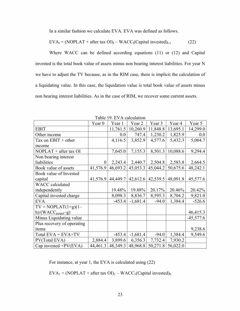
In a similar fashion we calculate EVA. EVA was defined as follows.
Where WACC can be defined according equations (11) or (12) and Capital
invested is the total book value of assets minus non bearing interest liabilities. For year N
we have to adjust the TV because, as in the RIM case, there is implicit the calculation of
a liquidating value. In this case, the liquidation value is total book value of assets minus
non bearing interest liabilities. As in the case of RIM, we recover some current assets.
Table 19. EVA calculation Year 0 Year 1 Year 2 Year 3 Year 4 Year 5 EBIT 11,761.5 10,260.9 11,848.8 13,695.1 14,299.0Other income 0.0 747.4 1,230.2 1,825.9 0.0Tax on EBIT + other income
4,116.5 3,852.9 4,577.6 5,432.3 5,004.7
NOPLAT + after tax OI 7,645.0 7,155.3 8,501.3 10,088.6 9,294.4Non bearing interest liabilities 0 2,243.4 2,440.7 2,504.8 2,583.8 2,664.5Book value of assets 41,576.9 46,693.2 45,053.3 45,044.2 50,675.6 48,242.1Book value of Invested capital 41,576.9 44,449.7 42,612.6 42,539.5 48,091.8 45,577.6WACC calculated independently 19.48% 19.88% 20.17% 20.46% 20.42%Capital invested charge 8,098.3 8,836.7 8,595.3 8,704.2 9,821.0EVA -453.4 -1,681.4 -94.0 1,384.4 -526.6TV = NOPLAT(1+g)(1–h)/(WACCperpet–g) 46,415.3Minus Liquidating value -45,577.6Plus recovery of operating items
9,238.6
Total EVA = EVA+TV -453.4 -1,681.4 -94.0 1,384.4 9,549.6PV(Total EVA) 2,884.4 3,899.6 6,356.3 7,732.4 7,930.2 Cap invested +PV(EVA) 44,461.3 48,349.3 48,968.8 50,271.8 56,022.0
For instance, at year 1, the EVA is calculated using (22)
EVA1 = (NOPLAT + after tax OI)1 – WACC1(Capital invested)0
24
EVA1 = 7,645.0 − 19.48% × 41,576.9
= 7,645.0 − 8,098.3 = -453.4
Observe again that the total value and equity market value are exactly the same as
the ones calculated with the DCF and RI methods.
As a final observation notice that the Net Present value of this firm is positive and
the fact that we have some RI or EVA with negative values do not mean anything
regarding the value of the project (firm). The important issue is to see the flows (EVA
and RI can be considered a flow, but not in the sense of cash flow) as a whole. This
means that an individual annual value of RI or EVA means nothing when assessing value.
Those individual values could be used to measure the managerial performance. However,
care has to be taken in the interpretation on the sign of those individual values. For
further analysis on this see Velez-Pareja 2000.
Section Four
Concluding Remarks We have shown not only that we get consistent results from the DCF methods
when calculating total and equity values, but we have shown that the RI and EVA
approaches gives exactly the same results when properly done and are consistent. In this
note we presented a complex example with finite cash flows and terminal value.
Bibliographic References Copeland, Thomas E., Koller, T. y Murrin, J., 2001, Valuation: Measuring and
Managing the Value of Companies, 3rd Edition, John Wiley & Sons. Ehrbar, Al, 1998, EVA., The Real Key to Creating Wealth, Wiley.
Fernandez, Pablo (2002) Valuation Methods and Shareholder Value Creation, Academic Press. Lundholm, Russell J. and Terry O'Keefe, 2001, Reconciling Value Estimates from
the Discounted Cash Flow Model and the Residual Income Model, Contemporary
25
Accounting Research. Summer. Can be downloaded with the same title as Working Paper from Social Science Research Network (www.ssrn.com). Posted 2001.
Ruback, Richard S. 2002, Capital Cash Flows: A Simple Approach to Valuing Risky Cash Flows, Financial Management, Vol. 31, No. 2, Summer. Can be downloaded with the same title as Working Paper from Social Science Research Network (www.ssrn.com). Posted 2000.
Stewart, III, G. Bennet, 1999, The Quest for Value, HerperBusiness. Tham, Joseph, 2000, Consistent Value Estimates from the Discounted Cash Flow
(DCF) and Residual Income (RI) Models in M & M Worlds Without and With Taxes. Can be downloaded with the same title as Working Paper from Social Science Research Network (www.ssrn.com). Posted 2000.
Tham, Joseph, 2001, Equivalence between Discounted Cash Flow (DCF) and Residual Income (RI), Working Paper, Social Science Research Network (www.ssrn.com).
Velez-Pareja, Ignacio, 2000, Economic Value Measurement: Investment Recovery and Value Added – IRVA, Working Paper, Social Science Research Network (www.ssrn.com).
Velez-Pareja, Ignacio, 1999, "Value Creation and its Measurement: A Critical Look to EVA", Working Paper, Social Science Research Network (www.ssrn.com). Spanish version in Cuadernos de Administración, N. 22, Junio 2000, pp.7-31.
Velez-Pareja, Ignacio and Joseph Tham, 2001, A Note on the Weighted Average Cost of Capital WACC, Working Paper, Social Science Research Network (www.ssrn.com). Spanish version in Monografías No 62, Serie de Finanzas, La medición del valor y del costo de capital en la empresa, de la Facultad de Administración de la Universidad de los Andes, julio 2002, pp. 61-98. and as Working Paper at Social Science Research Network (www.ssrn.com).
Young, S.David and Stephen F. O’Byrne, 2001, EVA and Value-Based Management, McGraw Hill.
26
Appendix
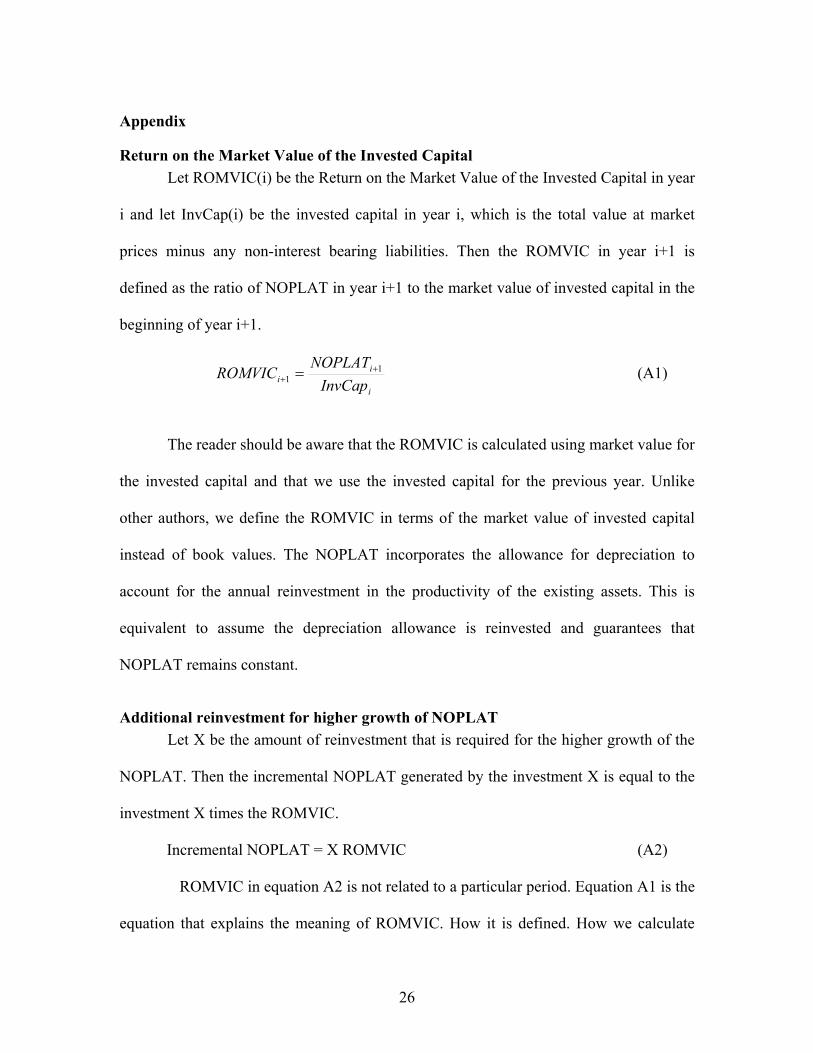
Return on the Market Value of the Invested Capital Let ROMVIC(i) be the Return on the Market Value of the Invested Capital in year
i and let InvCap(i) be the invested capital in year i, which is the total value at market
prices minus any non-interest bearing liabilities. Then the ROMVIC in year i+1 is
defined as the ratio of NOPLAT in year i+1 to the market value of invested capital in the
beginning of year i+1.
i
ii InvCap
NOPLATROMVIC 1
1+
+ = (A1)
The reader should be aware that the ROMVIC is calculated using market value for
the invested capital and that we use the invested capital for the previous year. Unlike
other authors, we define the ROMVIC in terms of the market value of invested capital
instead of book values. The NOPLAT incorporates the allowance for depreciation to
account for the annual reinvestment in the productivity of the existing assets. This is
equivalent to assume the depreciation allowance is reinvested and guarantees that
NOPLAT remains constant.
Additional reinvestment for higher growth of NOPLAT Let X be the amount of reinvestment that is required for the higher growth of the
NOPLAT. Then the incremental NOPLAT generated by the investment X is equal to the
investment X times the ROMVIC.
Incremental NOPLAT = X ROMVIC (A2)
ROMVIC in equation A2 is not related to a particular period. Equation A1 is the
equation that explains the meaning of ROMVIC. How it is defined. How we calculate
27
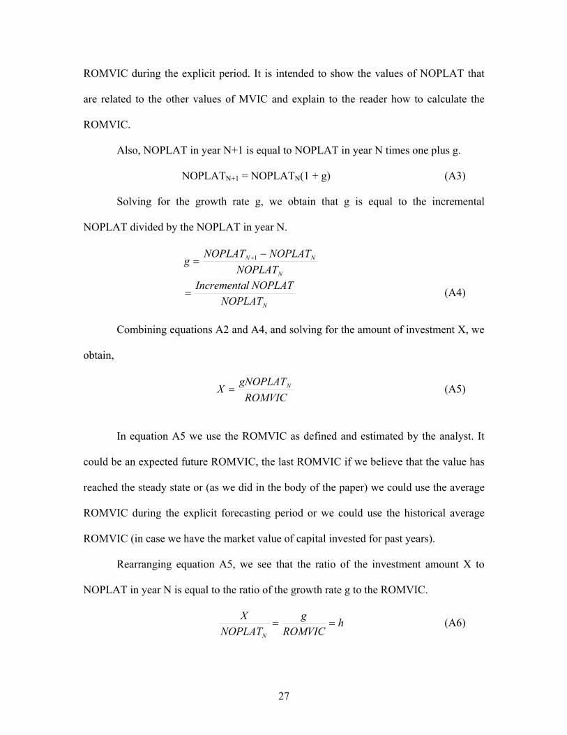
ROMVIC during the explicit period. It is intended to show the values of NOPLAT that
are related to the other values of MVIC and explain to the reader how to calculate the
ROMVIC.
Also, NOPLAT in year N+1 is equal to NOPLAT in year N times one plus g.
NOPLATN+1 = NOPLATN(1 + g) (A3)
Solving for the growth rate g, we obtain that g is equal to the incremental
NOPLAT divided by the NOPLAT in year N.
N
NN
NOPLATNOPLATNOPLAT
g−
= +1
NNOPLATNOPLATlIncrementa
= (A4)
Combining equations A2 and A4, and solving for the amount of investment X, we
obtain,
ROMVIC
gNOPLATX N= (A5)
In equation A5 we use the ROMVIC as defined and estimated by the analyst. It
could be an expected future ROMVIC, the last ROMVIC if we believe that the value has
reached the steady state or (as we did in the body of the paper) we could use the average
ROMVIC during the explicit forecasting period or we could use the historical average
ROMVIC (in case we have the market value of capital invested for past years).
Rearranging equation A5, we see that the ratio of the investment amount X to
NOPLAT in year N is equal to the ratio of the growth rate g to the ROMVIC.
hROMVIC
gNOPLAT
X
N
== (A6)
28
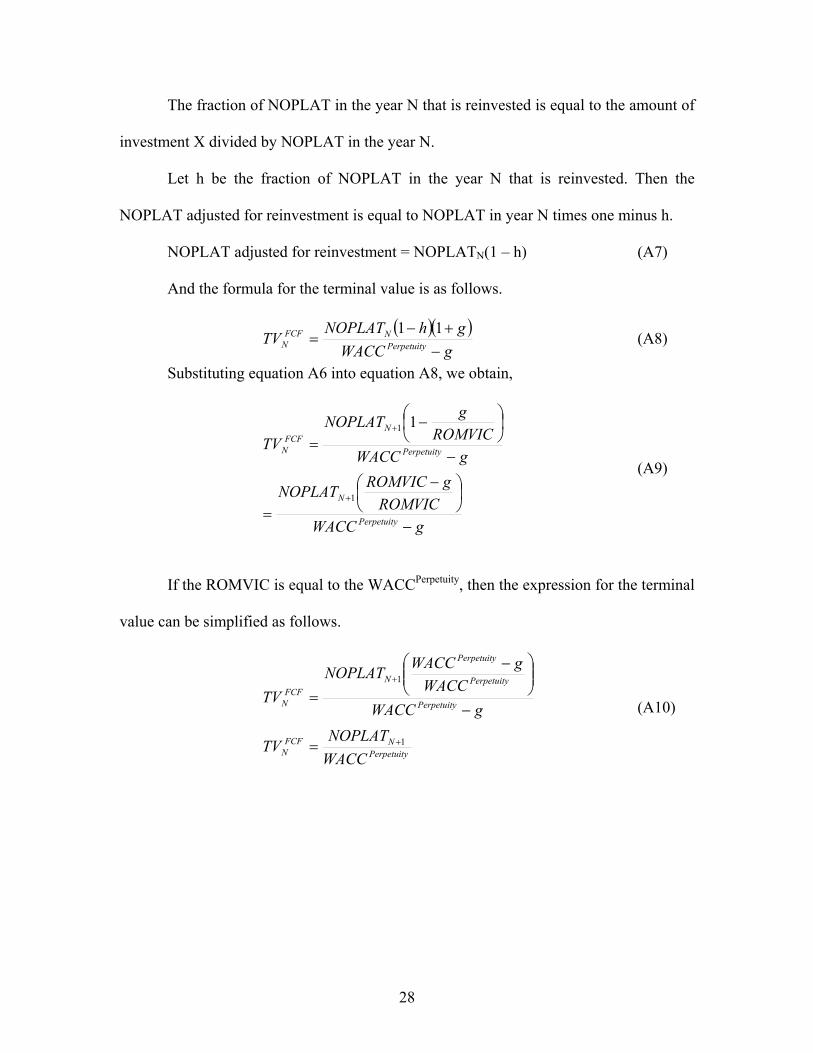
The fraction of NOPLAT in the year N that is reinvested is equal to the amount of
investment X divided by NOPLAT in the year N.
Let h be the fraction of NOPLAT in the year N that is reinvested. Then the
NOPLAT adjusted for reinvestment is equal to NOPLAT in year N times one minus h.
NOPLAT adjusted for reinvestment = NOPLATN(1 – h) (A7)
And the formula for the terminal value is as follows.
( )( )
gWACCghNOPLAT
TV PerpetuityNFCF
N −+−
=11
(A8)
Substituting equation A6 into equation A8, we obtain,
gWACCROMVIC
gROMVICNOPLAT
gWACCROMVIC
gNOPLATTV
Perpetuity
N
Perpetuity
NFCF
N
−
−
=
−
−
=
+
+
1
1 1
(A9)
If the ROMVIC is equal to the WACCPerpetuity, then the expression for the terminal