Page 1
Approved by and published under the authority of the Secretary General
INTERNATIONAL CIVIL AVIATION ORGANIZATION
Doc 9501
Environmental Technical Manual
Volume III — Procedures for the CO2 Emissions Certification of AeroplanesFirst Edition, 2018
vmuraca
Text Box
CAEP10 (February 2016) and CAEP Steering Group 2016 and 2017 approved revision (Based on the First Edition - 2017)
vmuraca
Text Box
CAEP STEERING GROUP 2016 AND 2017 APPROVED REVISION
Page 2
Published in separate English, Arabic, Chinese, French, Russian
and Spanish editions by the
INTERNATIONAL CIVIL AVIATION ORGANIZATION
999 Robert-Bourassa Boulevard, Montréal, Quebec, Canada H3C 5H7
For ordering information and for a complete listing of sales agents
and booksellers, please go to the ICAO website at www.icao.int
First edition, 2018
Doc 9501, Environmental Technical Manual
Volume III, Procedures for the CO2 Emissions Certification of Aeroplanes
Order Number: 9501-3
ISBN 978-92-9258-274-6
© ICAO 2018
All rights reserved. No part of this publication may be reproduced, stored in a
retrieval system or transmitted in any form or by any means, without prior
permission in writing from the International Civil Aviation Organization.
Page 3
(iii)
AMENDMENTS
Amendments are announced in the supplements to the Products and Services
Catalogue; the Catalogue and its supplements are available on the ICAO
website at www.icao.int. The space below is provided to keep a record of
such amendments.
RECORD OF AMENDMENTS AND CORRIGENDA
AMENDMENTS CORRIGENDA
No. Date Entered by No. Date Entered by
Page 5
(v)
FOREWORD
The Environmental Technical Manual (Doc 9501), Volume III — Procedures for the CO2 Emissions Certification of
Aeroplanes, First Edition, includes material that has been approved by the ICAO Committee on Aviation
Environmental Protection (CAEP) during their tenth meeting (CAEP/10) in February 2016. This manual is to be
periodically revised under the supervision of the CAEP Steering Group and is intended to make the most recent
information available to certificating authorities, aeroplane certification applicants and other interested parties in a
timely manner, aiming at achieving the highest degree of harmonization possible. The technical procedures and
equivalent procedures described in the manual are consistent with currently accepted techniques and modern
instrumentation. This edition and subsequent revisions that may be approved by the CAEP Steering Group will be
posted on the ICAO website (http://www.icao.int/) under “publications” until the latest approved revision is submitted
to CAEP for formal endorsement and subsequent publication by ICAO.
Comments on this manual, particularly with respect to its application and usefulness, would be appreciated from all
States. These comments will be taken into account in the preparation of subsequent editions. Comments concerning this
manual should be addressed to:
The Secretary General
International Civil Aviation Organization
999 Robert-Bourassa Boulevard
Montréal, Quebec H3C 5H7
Canada
______________________
Page 7
(vii)
TABLE OF CONTENTS
Page
Acronyms and abbreviations ......................................................................................................................... (ix)
Chapter 1. Introduction ............................................................................................................................... 1-1
1.1 Purpose .......................................................................................................................................... 1-1
1.2 Document structure ........................................................................................................................ 1-1
1.3 Equivalent procedures .................................................................................................................... 1-1
1.4 Explanatory information ................................................................................................................ 1-2
1.5 Conversion of units ........................................................................................................................ 1-2
1.6 References ...................................................................................................................................... 1-2
Chapter 2. General guidelines ..................................................................................................................... 2-1
2.1 Applicability of Annex 16, Volume III .......................................................................................... 2-1
2.2 Changes to CO2-approved aeroplane type designs......................................................................... 2-3
2.3 CO2 emissions evaluation metric compliance demonstration plans ............................................... 2-4
2.4 Engine intermix .............................................................................................................................. 2-5
2.5 Exemptions .................................................................................................................................... 2-6
Chapter 3. SAR determination procedures ............................................................................................... 3-1
3.1 SAR measurement procedures ....................................................................................................... 3-1
3.2 SAR data analysis .......................................................................................................................... 3-2
3.3 Validity of results - confidence interval ......................................................................................... 3-14
3.4 Equivalent procedures .................................................................................................................... 3-34
Appendix 1. References ............................................................................................................................... App 1-1
Appendix 2. Bibliography ............................................................................................................................ App 2-1
______________________
Page 9
(ix)
ACRONYMS AND ABBREVIATIONS
A Area (m2)
CAEP Committee on Aviation Environmental Protection
CD Drag coefficient
CFD Computational fluid dynamics
CG Centre of gravity
CI Confidence interval
CL Lift coefficient
CO2 Carbon dioxide
g Gravitational acceleration (m/s2)
h Altitude (m)
LHV Lower heating value (MJ/kg)
M Mach number
MAC Mean aerodynamic chord (cm)
MTOM Maximum take-off mass (kg)
Re Radius of the Earth (m)
RE Reynolds number
RGF Reference geometric factor
SAR Specific air range (km/kg)
SFC Specific fuel consumption
STC Supplemental type certificate
T Temperature (K)
TAS True airspeed (km/h)
TC Type certificate
TOM Take-off mass (kg)
V Speed (m/s)
Wf Total aeroplane fuel flow (kg/h)
W Weight (N)
WV Weight variant
δ Ratio of atmospheric pressure at a given altitude to the atmospheric pressure at sea level
Φ Latitude degrees
ρ Density (kg/m3)
σ Ground track angle degrees
______________________
Page 11
1-1
Chapter 1
INTRODUCTION
1.1 PURPOSE
The aim of this manual is to promote uniformity in the implementation of the technical procedures of Annex 16 —
Environmental Protection, Volume III — Aeroplane CO2 Emissions by providing: 1) guidance to certificating
authorities, applicants and other interested parties regarding the intended meaning and stringency of the Standards in
the current edition of the Annex; 2) guidance on specific methods that are deemed acceptable in demonstrating
compliance with those Standards; and 3) equivalent procedures resulting in effectively the same CO2 emissions
evaluation metric that may be used in lieu of the procedures specified in the appendices of Annex 16, Volume III.
1.2 DOCUMENT STRUCTURE
1.2.1 Chapter 1 provides general information regarding the use of this manual. Chapter 2 provides general
guidelines on the interpretation of Annex 16, Volume III. Chapter 3 brings technical guidelines for the certification of
aeroplanes against Annex 16, Volume III, including equivalent procedures.
1.2.2 Guidance is provided in the form of explanatory information, acceptable methods for showing compliance,
and equivalent procedures.
1.3 EQUIVALENT PROCEDURES
1.3.1 The procedures described in the Annex, as supplemented by the means of compliance information
provided in this manual, shall be used unless an equivalent procedure is approved by the certificating authority.
Equivalent procedures should not be considered as limited only to those described herein, as this manual will be
expanded as new equivalent procedures are developed. Also, their presentation does not imply limitation of their
application or commitment by certificating authorities to their further use.
1.3.2 The use of equivalent procedures may be requested by applicants for many reasons, including:
a) to make use of previously acquired or existing data for the aeroplane; and
b) to minimize the costs of demonstrating compliance with the requirements of Annex 16, Volume III,
by keeping aeroplane test time and equipment and personnel costs to a minimum.
Page 12
1-2 Environmental Technical Manual
1.4 EXPLANATORY INFORMATION
Explanatory information has the following purpose:
a) to explain the intent of the Annex 16 Volume III Standards;
b) to state current policies of certificating authorities regarding compliance with the Annex; and
c) to provide information on critical issues concerning approval of applicants’ compliance methodology
proposals.
1.5 CONVERSION OF UNITS
Conversions of some non-critical numerical values between U.S. Customary (English) and SI units are shown in the
context of acceptable approximations.
1.6 REFERENCES
1.6.1 Unless otherwise specified, references throughout this document to “the Annex” relate to Annex 16 —
Environmental Protection, Volume III — Aeroplane CO2 Emissions, First Edition.
1.6.2 References to sections of this manual are defined only by the section number to which they refer.
References to documents other than the Annex are numbered sequentially (e.g., Reference 1, Reference 2, etc.). A list
of these documents is provided in Appendix 1 of this manual, and a bibliography can be found in Appendix 2.
______________________
Page 13
2-1
Chapter 2
GENERAL GUIDELINES
2.1 APPLICABILITY OF ANNEX 16, VOLUME III
2.1.1 The Convention on International Civil Aviation, Article 3, specifically states that it is not applicable to
state aircraft and provides some examples (see below), but this can also include specific flights carrying official
government representatives:
“a) This Convention shall be applicable only to civil aircraft, and shall not be applicable to state aircraft.
b) Aircraft used in military, customs and police services shall be deemed to be state aircraft.”
2.1.2 In addition, Annex 16, Vol. III, Part II, Chapter 2, 2.1 excepts amphibious aeroplanes, aeroplanes initially
designed or modified for specialized operational requirements and used as such, aeroplanes designed with zero
reference geometric factor (RGF), and those aeroplanes specifically designed or modified and used for fire-fighting
purposes. These are typically special categories of aeroplanes which are limited in numbers and have specific technical
characteristics resulting in very different CO2 metric values compared to all other aeroplane types in the proposed
applicability scope.
2.1.3 Examples of specialized operational requirements include:
a) aeroplanes that are initially certified as civil aeroplanes during the production process but
immediately converted to military aeroplanes;
b) a required capacity to carry cargo that is not possible by using less specialized aeroplanes (e.g.
ramped, with back cargo door);
c) a required capacity for very short or vertical take-offs and landings;
d) a required capacity to conduct scientific, research or humanitarian missions exclusive of commercial
service; or
e) similar factors.
2.1.4 Type design configurations which shall be certified
2.1.4.1 Annex 16, Volume III, Part I, Chapter 1, defines maximum take-off mass (MTOM) as “the highest of all
take-off masses for the type design configuration”. Part II, Chapter 2, 2.3, defines the three reference masses at which
the 1/SAR value shall be established, and these masses are calculated based on the MTOM.
2.1.4.2 Applicants may develop multiple take-off mass (TOM) variants of a specific type design configuration
(i.e. combination of airframe/engine) for operational purposes. As stated above, only the highest MTOM of a specific
airframe/engine combination is required to be certified against Annex 16, Volume III. As stated in Annex 16,
Volume III, Part II, Chapter 2, 2.3.2, certification at MTOM also certifies all TOM variants. These TOM variants
Page 14
2-2 Environmental Technical Manual
would have the same CO2 emissions evaluation metric value as MTOM.
2.1.4.3 Annex 16, Volume III, Part II, Chapter 2, 2.3.2, also states that “applicants may voluntarily apply for the
approval of CO2 metric values for take-off masses less than MTOM.” The purpose of this statement is to allow the
applicant to apply for approval of a separate CO2 emissions evaluation metric value for a TOM lower than MTOM. In
that case, the reference aeroplane masses and the maximum permitted CO2 emissions evaluation metric value would be
based on the TOM instead of MTOM. The CO2 emissions evaluation metric value for this TOM could then also be
used for any TOM variant of even lower mass. Applicants can apply for approval for separate CO2 emissions
evaluation metric values for as many or as few TOM variants as they desire.
2.1.4.4 Example of type design configurations to be certified
2.1.4.4.1 Assuming an applicant applies for the approval of the following type design configurations:
a) two fuselage lengths: Model A and Model B;
b) two engine options: Engine X and Engine Y;
c) two weight variants (WV) for each fuselage length: WV01 and WV02 for Model A and WV11 and
WV12 for Model B.
The possible combinations are summarized in Table 2-1.
Table 2-1. Type design configuration combinations
Model A
Engine X WV01
WV02
Engine Y WV01
WV02
Model B
Engine X WV11
WV12
Engine Y WV11
WV12
2.1.4.4.2 The type design configurations that shall be certified against Annex 16, Volume III, are the ones that have
the highest MTOM. Each combination of fuselage length and engine option is a separate type design configuration.
Assuming WV01 and WV11 have higher MTOMs than WV02 and WV12, the following combinations shall be
certified:
a) Model A — Engine X – WV01;
b) Model A — Engine Y – WV01;
Page 15
Volume III. Procedures for the CO2 Emissions Certification of Aeroplanes
Chapter 2 2-3
c) Model B — Engine X – WV11;
d) Model B — Engine Y – WV11.
2.1.4.4.3 The combinations with WV02 and WV12 would be assigned the same CO2 emissions evaluation metric
value as the combinations with WV01 and WV11, respectively. At the applicant’s option, the combinations with WV02
and/or WV12 could also be certified to obtain a different CO2 emissions evaluation metric value for those combinations.
2.1.5 Appropriate margin to regulatory level
2.1.5.1 If an applicant chooses to voluntarily certify a lower TOM variant, as discussed in 2.1.4, it should be kept
in mind that an underlying principle in applying the CO2 standard is that the highest weight variant (MTOM) has the
lowest margin to the regulatory limit level. The 1/SAR value used in the CO2 metric system is calculated as an average
of three reference masses (high, medium and low).
2.1.5.2 In establishing the reference conditions for specific air range (SAR) determination, it is expected that the
highest SAR value will be sought at the maximum range cruise condition at the optimum altitude (Annex 16,
Volume III, Chapter 2, 2.5). It is noted that a greater non-linearity in the 1/SAR versus mass relationship could be
introduced by a constraint unrelated to the aerodynamic and propulsive efficiency of the aeroplane (e.g. an altitude
pressurization limitation). In this instance, particular care should be taken to ensure that that the principle of the highest
weight variant having the lowest margin to the regulatory limit level continues to hold.
2.2 CHANGES TO CO2-APPROVED AEROPLANE TYPE DESIGNS
2.2.1 Annex 16, Volume III, Part I, Chapter 1, includes the following definition:
“Derived version of a CO2-certified aeroplane. An aeroplane which incorporates changes in
type design that either increase its maximum take-off mass, or that increase its CO2 emissions
evaluation metric value by more than:
a) 1.35 per cent at a maximum take-off mass of 5 700 kg, decreasing linearly to;
b) 0.75 per cent at a maximum take-off mass of 60 000 kg, decreasing linearly to;
c) 0.70 per cent at a maximum take-off mass of 600 000 kg; and
d) a constant 0.70 per cent at maximum take-off masses greater than 600 000 kg.
Note.— In some States, where the certificating authority finds that the proposed change in
design, configuration, power or mass is so extensive that a substantially new investigation of
compliance with the applicable airworthiness regulations is required, the aeroplane will be
considered to be a new type design rather than a derived version.”
2.2.2 The note clarifies that it is the airworthiness regulations that determine whether or not an aeroplane model
is a New Type design (ref. ANAC RBAC 21.19, EASA Part 21.A.19, FAA: Title 14 of the Code of Federal
Regulations, Chapter I, Subchapter C, Part 21.19, IAC AP-21 Subpart B para. 21/19, TCCA CAR 521.153). If it is a
New Type for airworthiness, then it is also a New Type design from CO2 emissions certification perspective.
Conversely, if the airworthiness requirements do not determine an aeroplane model to be a New Type, then it is a
Page 16
2-4 Environmental Technical Manual
Derived Version for the CO2 requirements. In this case the CO2 certification basis is the same as the aeroplane model
from which it is derived, or any later amendment at the option of the applicant.
2.2.3 Consequently, any change to a CO2-certified aeroplane type design that increases its MTOM shall be
considered a derived version, and the applicant shall demonstrate compliance with Annex 16, Volume III. In addition,
any change to a CO2-certified aeroplane type design that increases its certified CO2 emissions evaluation metric value
by more than the above-mentioned thresholds shall be considered a derived version, and the applicant shall demonstrate
compliance with Annex 16, Volume III.
2.2.4 Changes to a CO2-certified aeroplane type design that do not increase its MTOM or its CO2 emissions
evaluation metric by more than the above-mentioned thresholds are considered no-CO2 changes, and the CO2 emissions
evaluation metric value of the changed type design configuration shall be considered the same as the parent type design.
This definition of the no-CO2 change thresholds is also referred to as the “no-CO2-change criterion”.
2.2.5 The evaluation of certain changes can be done by simpler equivalent procedures, as detailed in 3.4.2 and 3.4.3.
2.2.6 Visualization of the no-CO2-change criterion thresholds is provided in Figure 2-1. The trend line
equations may be used to evaluate what the no-CO2 change threshold is for any MTOM.
Figure 2-1. Visualization of the no-CO2-change criterion
1.5%
1.2%
0.9%
0.6%
0.3%
1.5%
0 100 000 200 000 300 000 400 000 500 000 600 000 700 000
No-
CO
-ch
an
ge
crite
rio
n p
erc
en
t va
lue
2
No-CO -change criterion2
No-CO -change criterion threshold21.35%, 5 700 kg
0.75%, 60 000 kg
y = 1.10497E-07x + 1.41298E-02
y = -9.25926E-10x + 7.55556E-03 y = 7.00E-03
0.70%, 600 000 kg
Maximum take-off mass (kg)
Page 17
Volume III. Procedures for the CO2 Emissions Certification of Aeroplanes
Chapter 2 2-5
2.3 CO2 EMISSIONS EVALUATION METRIC
COMPLIANCE DEMONSTRATION PLANS
Prior to undertaking a CO2 certification demonstration, the applicant should submit to the certificating authority a CO2
compliance demonstration plan. This plan contains a complete description of the methodology and procedures by
which an applicant proposes to demonstrate compliance with the CO2 certification Standards specified in Annex 16,
Volume III. Approval of the plan and the proposed use of any equivalent procedures or technical procedures not
included in the Annex remains with the certificating authority. CO2 compliance demonstration plans should include the
following information:
a) Introduction. A description of the aeroplane CO2 certification basis.
b) Aeroplane description. Type, model number and the specific configuration to be certificated.
Note.— The certificating authority should require that the applicant demonstrate and document the
conformity of the test aeroplane, particularly with regard to those parts which might affect its CO2
emissions evaluation metric.
c) Aeroplane CO2 certification methodology. Means of compliance, equivalent procedures from this
manual, and technical procedures from Annex 16, Volume III.
d) Plans for tests. The plans for test should include:
1) Test description. Test methods to comply with the test environment and flight path conditions of
the Annex, as appropriate.
Note.— Plans for tests shall either be integrated into the basic CO2 compliance demonstration plan
or submitted separately and referenced in the basic plan.
e) Deliverables. List the documents that should show compliance with Annex 16, Volume III (test and
analysis reports, including RGF determination).
2.4 ENGINE INTERMIX
2.4.1 Applicants will typically demonstrate compliance with the Standards in Annex 16, Volume III, Chapter 2,
for an aeroplane type configuration where all engines are of the same design. However, an applicant may wish to
demonstrate compliance of an aeroplane type configuration where not all the engines are of the same design. Such a
configuration is commonly referred to as an “engine intermix” configuration.
2.4.2 In such a case, the applicant may, subject to the approval of the certificating authority, demonstrate
compliance in one of three ways:
a) in accordance with the test procedures defined in Annex 16, Volume III, Chapter 2, 2.6, and for
which the test aeroplane shall be representative of the intermix configuration for which certification
is requested; or
b) in cases where the CO2 metric value has been established for aeroplanes on which each of the
intermix engine models has been exclusively installed, compliance can be demonstrated on the basis
of either:
Page 18
2-6 Environmental Technical Manual
1) the average of the CO2 emissions evaluation metrics for aeroplanes on which each of the
intermix engine models has been exclusively installed; or
2) the highest CO2 emissions evaluation metric for aeroplanes on which each of the intermix engine
models has been exclusively installed.
Note.— Annex 16, Volume III, Chapter 2, 2.1.2, states that in the case of time-limited engine changes,
Contracting States may not require a demonstration of compliance with the Standards of Annex 16, Volume III.
2.5 EXEMPTIONS
2.5.1 Introduction
2.5.1.1 Annex 16, Volume III, Part II, Chapter 2, 2.1.3 raises the possibility for certificating authorities to exempt
aeroplane units from the applicability requirements in the First Edition of Annex 16, Volume III, Part II, Chapter 2,
2.1.1 (a) to (g).
2.5.1.2 In addition Part II, Chapter 1, 1.11, indicates that Contracting States shall recognise valid exemptions
agreed by another Contracting State provided that the process for granting exemption is acceptable. It is recommended
to follow the acceptable process and criteria as described in this ETM. For example, certificating authorities may
decide to exempt low volume production aeroplanes in exceptional circumstances, taking into account the justifications
listed in 2.5.2.1 c).
2.5.1.3 In order to promote a harmonized global approach to the granting, implementing and monitoring of these
exemptions, this section provides guidelines on the process and criteria for issuing exemptions from the CO2 Standard
agreed at CAEP/10 (Part II, Chapter 2, 2.4).
2.5.2 Exemption process
2.5.2.1 Application
In order for the competent authority to review an application, the applicant should submit to the competent authority a
formal application letter for the manufacture of the exempted aeroplanes, with a copy to all other relevant organizations
and involved competent authorities. The letter should include the following information in order for the competent
authority to be in a position to review the application:
a) Administration
1) name, address and contact details of the applicant.
b) Scope of application for exemptions
1) aeroplane type (e.g. new or in-production type, model designation, type certificate (TC) number
and TC date);
2) number of aeroplane exemptions requested;
3) anticipated duration (end date) of continued production of exempted aeroplanes;
Page 19
Volume III. Procedures for the CO2 Emissions Certification of Aeroplanes
Chapter 2 2-7
4) designation of to whom the aeroplanes will be originally delivered.
c) Justification for the exemptions. In applying for an exemption, an applicant should, to the extent
possible, address the following factors (with quantification) in order to support the merits of the
exemption request:
1) technical issues from an environmental and airworthiness perspective which may have delayed
compliance;
2) economic impacts on the manufacturer, operator(s) and the aviation industry at large;
3) environmental effects. This should consider the amount of additional CO2 that will be emitted as
a result of the exemption, including items such as the amount by which the aeroplane model
exceeds the Standard, taking into account any other aeroplane models in the aeroplane family
covered by the same type certificate and their relation to the Standard;
4) interdependencies. The impact of changes to reduce CO2 on other environmental factors,
including community noise and NOx emissions;
5) the impact of unforeseen circumstances and hardship due to business circumstances beyond the
manufacturer’s control (e.g. employee strike, supplier disruption or calamitous event);
6) projected future production volumes and plans for producing a compliant version of the
aeroplane model for which exemptions are sought;
7) for NT aeroplanes only, provide a demonstration that the maximum use of fuel efficient
technology relative to CAEP/10 NT regulatory limit was reasonably applied to the design to the
aeroplane;
8) equity issues in granting exemptions among economically competing parties (e.g. provide the
rationale for granting an exemption when another manufacturer has a compliant aeroplane and
does not need an exemption, taking into account the implications for operator fleet composition,
commonality and related issues in the absence of the aeroplane for which exemptions are
sought); and
9) any other relevant factors.
2.5.2.2 Evaluation criteria
2.5.2.2.1 The evaluation of an exemption application should be based on the justification provided. The total
number of exempted aeroplanes should be agreed at the time the application is approved and based on the
considerations explained in 2.5.2.1 c).
2.5.2.2.2 The proposed maximum number of potential exemptions should be inversely proportional to the %
margin of the CO2 metric value from the regulatory level (Part II, Chapter 2, 2.4). Those aeroplane types with a
smaller % margin to the regulatory level should be permitted a larger number of exemptions compared to the aeroplane
types with a larger % margin.
2.5.2.2.3 Following the recommendation in Part II, Chapter 1, 1.11 to use an acceptable process, the number of
aeroplanes exempted per type certificate would normally not exceed the proposed maximum number in the tables and
Page 20
2-8 Environmental Technical Manual
figures below.
% Margin to CAEP10
In-Production Regulatory level Maximum Exemptions Total
0 to 2 75
>2 to 10 -7.5 x (per cent margin to CAEP10 regulatory level)+90
More than 10 15
Figure 2-2. The graphical representation of InP exemptions for the CAEP/10 Aeroplane CO2
Emissions Standard
Page 21
Volume III. Procedures for the CO2 Emissions Certification of Aeroplanes
Chapter 2 2-9
% Margin to CAEP10
New Type Regulatory level Maximum Exemptions Total
0 to 2 40
>2 to 4 -20 x (percent margin to CAEP10 regulatory level)+80
More than 4 0
Figure 2-3. The graphical representation of NT exemptions for the CAEP/10 Aeroplane CO2
Emissions Standard
2.5.2.2.4 The maximum number of exemptions should be reviewed during the CAEP/13 cycle (2022 – 2025).
Page 22
2-10 Environmental Technical Manual
2.5.2.3 Review
The competent authority should review, in a timely manner, the application using the information provided in 2.5.2.1
and the evaluation criteria in 2.5.2.2. The analysis and conclusions from the review should be communicated to the
applicant through a formal response. If the application is approved, the response should clearly state the scope of the
exemptions that have been granted. If the application is rejected, the response should include a detailed justification.
2.5.3 Registration and communication
Oversight of the granted exemptions should include the following elements:
a) The competent authority should publish details of the exempted aeroplanes in an official public
register, including aeroplane model and maximum number of permitted exemptions.
b) The applicant should have a quality control process for maintaining oversight of and managing the
production of aeroplanes which have been granted exemptions.
c) An exemption should be recorded in the aeroplane statement of conformity1 which states conformity
with the type certificate (proposed standard text: “Aeroplane exempted from the First Edition of
Annex 16, Volume III, Chapter 2, 2.1.1 [x]2”).
d) The applicant should provide to the competent authority, on a regular basis and appropriate to the
limitation of the approval, details on the actual exempted aeroplanes which have been produced
(e.g. model, aeroplane type and serial number).
e) Exemptions for new aeroplanes should be processed and approved by the competent authority for the
production of the exempted aeroplanes in coordination with the competent authorities responsible for
the design of the aeroplane and the issuance of the initial certificate of airworthiness.
______________________
1. For example: European Aviation Safety Agency (EASA) Form 52, United States Federal Aviation Administration (FAA) Form 8130-4 or
equivalent forms from other competent authorities. 2. Relevant applicability paragraph letter (a to g) would need to be filled for the exempted aeroplane.
Page 23
3-1
Chapter 3
SAR DETERMINATION PROCEDURES
3.1 SAR MEASUREMENT PROCEDURES
3.1.1 Flight test procedures
3.1.1.1 Fuel properties
3.1.1.1.1 One of the important factors when determining the CO2 emissions of an aeroplane according to Annex 16,
Volume III, is the fuel used in the flight tests.
3.1.1.1.2 Annex 16, Volume III, Part II, Chapter 2, 2.6.3, states: “Note.— The fuel used for each flight test should
meet the specification defined in either ASTM D1655-15, DEF STAN 91-91 Issue 7, Amendment 3, or equivalent.”
Equivalent fuel specifications accepted for the purposes of CO2 emissions certification are the following:
a) Brazil: CNP-08, QAV-1;
b) China: GB6537 Number 3 Jet Fuel;
c) France: DCSEA 134;
d) Russia: GOST 10227-86 or 52050-2006, RT;
e) USA: ASTM International D16551 entitled Standard Specification for Aviation Turbine Fuels;
f) UK: DEF STAN 91-912 entitled Turbine Fuel, Kerosene Type, Jet A-1;
g) Similar specifications from other member states, subject to the approval of the certificating authority.
3.1.1.1.3 The Annex, Part II, Chapter 2, 2.5.1, specifies the reference conditions to which the test conditions shall
be corrected. The reference fuel lower heating value is specified as 43.217 MJ/kg (18 580 BTU/lb). Appendix 1,
3.2.1 c), Recommendation 1), states that the fuel lower heating value should be determined in accordance with methods
that are at least as stringent as ASTM International D4809-09A3 entitled Standard Test Method for Heat of Combustion
of Liquid Hydrocarbon Fuels by Bomb Calorimeter (Precision Method). This method is estimated to have an accuracy
level of the order of 0.23 per cent.
3.1.1.1.4 The Annex, Appendix 1, 3.2.1 d), states that “a sample of fuel shall be taken for each flight test to
determine its specific gravity and viscosity when volumetric fuel flow meters are used”. The fuel’s specific gravity and
viscosity need not be determined if volumetric fuel flow meters are not used.
Page 24
3-2 Environmental Technical Manual
3.1.1.1.5 Examples of acceptable methods to determine the fuel’s specific gravity and viscosity are ASTM
International D40524 entitled Standard Test Method for Density and Relative Density of Liquids by Digital Density
Meter and ASTM International D4455, entitled Standard Test Method for Kinematic Viscosity of Transparent and
Opaque Liquids (and Calculation of Dynamic Viscosity). Other methods may be used subject to the approval of the
certificating authority.
3.2 SAR DATA ANALYSIS
3.2.1 Data selection
Selection of data used to show compliance to the Standard encompasses both the selection of flight test data gathered
during each test condition used to obtain an individual SAR point, as well as the distribution of the resulting corrected
SAR points in relation to the three reference masses and the reference conditions.
3.2.1.1 Selection of flight test data
3.2.1.1.1 There are multiple methods employed by aeroplane manufacturers in selecting flight test data for analysis,
reflecting a variety of tools and practices. Whichever method is chosen, the flight test data encompassed within the
selected range of time is expected to meet the stability criteria detailed in Annex 16, Volume III, Appendix 1, 3.2.3.1,
or alternative stability criteria approved by the certificating authority as per 3.2.3.2. Test data that do not meet these
stability criteria should normally be discarded. However, if such test data appear to be valid when compared with data
that meet the stability criteria, and the overall stability of the conditions is reasonably bounded, these data can be
retained, subject to the approval of the certificating authority.
3.2.1.1.2 One acceptable method is to employ an algorithm that automatically selects the data that meet all the
stability criteria, and discards data that do not. This method could be used to select the longest possible duration SAR
point that meets the required stability criteria, or to select multiple SAR points of the minimum requirement duration
(one minute), providing these points are separated by a minimum of two minutes or by an exceedance of the stability
criteria as specified in Annex 16, Volume III, Appendix 1, 3.2.2.2. Using a defined algorithm to select data in an
automated process allows repeatable and consistent application to other SAR points. This method may also yield a
greater number of SAR points to be used in defining the CO2 metric value and should represent a good statistical
distribution. However, because the amount of test data included in each SAR point is maximized, the resulting SAR
points could exhibit more scatter than if additional selection criteria are used.
3.2.1.1.3 Another method is to more closely examine the collected flight test data and select the timeframe to be
used to define the SAR point, by choosing the best or most stable data available and ignoring less stable data that
technically still meet the stability criteria. Examples of this are presented in Figures 3-1 and 3-2.
3.2.1.1.4 Figure 3-1 shows that the plotted parameters stay within the tolerances allowed by the stability criteria for
the duration of the test condition (the changing altitude after the end of the condition reflects pilot input to leave steady
flight and transition to the next test condition.). While all parameters are within the required tolerances, fluctuations in
ambient temperature and Mach are evident. Figure 3-2 shows the same data, but with a manually selected range of
shorter duration where the parameters are more stable.
3.2.1.1.5 Selecting data that meet more demanding stability criteria, instead of using all data that meet the stability
criteria indicated in Annex 16, Volume III, may allow the applicant to filter out observed instabilities caused by air
quality, changing environmental conditions, flight control inputs and aeroplane system dynamics. This could result in a
SAR point that is actually more representative of actual aeroplane performance.
Page 25
Volume III. Procedures for the CO2 Emissions Certification of Aeroplanes
Chapter 3 3-3
3.2.1.1.6 Whichever approach is taken to select data to define SAR points, it is important that the methodology be
applied as consistently as possible to minimize potential unseen bias in the resulting distribution of SAR points.
3.2.1.1.7 Another important aspect to consider when selecting data is to ensure that the time interval chosen is
representative of the aeroplane’s performance, and not indicative of a larger trend. For example, the first plot in
Figure 3-3 shows a trend line drawn through ground speed data over a 60-second time interval. This ground speed data
meets the stability criteria, and taken alone would indicate the need for an energy correction. However, if the ground
speed data trace was continued over a longer time interval, it becomes apparent that it exhibits cyclic behaviour. Cyclic
data need not be discarded necessarily, but the applicant should ensure that an appropriate time interval is selected such
that the arithmetic average is representative. In the example shown in Figure 3-3, an energy correction would be
inappropriate.
Figure 3-1. Flight test data time interval selection – Example 1
Mach Ground speed (km/hr) OAT ( C)° ALT (m)
+.005
-.005+3.7
-3.7+1
-1+23
-23
0 60 120 180
Time (s)
Test point duration = 2:40
Page 26
3-4 Environmental Technical Manual
Figure 3-2. Flight test data time interval selection – Example 2
-.005+3.7
-3.7+1
-1+23
-23
Mach Ground speed (km/hr) OAT ( C)° ALT (m)
+.005
-.005
0 60 120 180
Time (s)
Test point duration = 1:00
Page 27
Volume III. Procedures for the CO2 Emissions Certification of Aeroplanes
Chapter 3 3-5
Figure 3-3. Cyclic behaviour example
3.2.1.2 Distribution of resulting SAR points
3.2.1.2.1 Once the individual SAR points have been selected and corrected to reference conditions, they should be
examined to ensure they present an accurate representation of aeroplane performance.
3.2.1.2.2 For example, if direct flight test is being used to collect 6 SAR points targeting one reference mass, those
6 points when corrected to reference conditions should result in a reasonable grouping. If 5 of the points form a
reasonable grouping and one point is a clear outlier, the offending point may require closer scrutiny to ensure it is
actually representative. In such a situation, collection of additional data may be warranted, or, if appropriate, and
subject to the approval of the certificating authority, the offending data point could be discarded.
3.2.1.2.3 If the applicant conducts tests across a range of weights to build a regression line of SAR versus weight,
the collected SAR points should be reasonably distributed across the weight range. If a large portion of the regression
line is unsupported by data, or is anchored by a single SAR point, then the SAR determined for one of the reference
masses may be suspect. This is an important aspect to consider during the development of the certification plan and
flight test programme. As with the direct test method, if a single SAR point appears to be an outlier compared to the
rest of the data points, it should be examined more closely and could potentially be discarded.
Time (s)
Ground speed (km/hr) Linear best fit
2
0
-2
0 60 120 180 240
Ground speed (km/hr)
Linear best fit
2
0
-2
0 60
Time (s)
Page 28
3-6 Environmental Technical Manual
3.2.1.2.4 The applicant should investigate the collection of SAR points for potential sources of unintended bias, for
example, if all of the data points collected were during periods where groundspeed was increasing. If all of the test
points require a large energy correction in one direction, resulting in all SAR points being significantly increased
(or decreased), further scrutiny may be required to ensure a bias is not introduced, depending on the test data and
correction techniques being used.
3.2.2 Corrections to reference conditions
3.2.2.1 General. The guidance provided here represents one set of methods, but not the only acceptable methods,
for correcting the SAR test data to the reference conditions specified in Annex 16, Volume III, Part II, Chapter 2, 2.5.
3.2.2.1.1 Care needs to be taken not to inadvertently account for a correction twice when making any of the
corrections below. For example, when adjusting to the reference Mass/δ from the test Mass/δ, a drag correction is
introduced to account for the change in lift coefficient (CL). This change in CL, at a constant Mach number, also
changes the reference Reynolds number (RE) and the reference mass. However, these additional changes may already
be accounted for in the drag adjustments for off-nominal RE and aeroelastics depending on the correction methods used.
3.2.2.1.2 The corrections identified in paragraphs 3.2.2.2 through 3.2.2.12 cover corrections that should be made to
the tested values of aeroplane mass, drag and fuel flow. These corrected values of aeroplane mass, drag and fuel flow
should then be used to determine SAR for the reference conditions in the following manner, as per 3.2.2.1.2.1 to
3.2.2.1.2.4:
3.2.2.1.2.1 Determine the aeroplane mass corrected to reference conditions as per 3.2.2.2. Use this mass as the
reference mass outlined in 3.2.2.3.2 and 3.2.2.4.1, and as the mass for determining the aeroplane drag indicated in
3.2.2.1.2.2.
3.2.2.1.2.2 Determine the aeroplane drag for the test condition using the mass corrected for gravitational acceleration.
Determine all of the drag corrections as indicated in 3.2.2.3, 3.2.2.4, 3.2.2.5, 3.2.2.6 and 3.2.2.7. Sum these drag
corrections and add to the aeroplane drag for the test condition to obtain the aeroplane drag corrected to the reference
conditions.
3.2.2.1.2.3 Use the drag level corrected to reference conditions as per 3.2.2.1.2.2 as a thrust level (thrust = drag) to
determine the total engine fuel flow for these conditions from an engine performance model. Correct this engine fuel
flow to reference conditions indicated in 3.2.2.8, 3.2.2.9, 3.2.2.10, 3.2.2.11 and 3.2.2.12.
3.2.2.1.2.4 The SAR value corrected to reference conditions is given by the following relationship:
𝑆𝐴𝑅𝑟𝑒𝑓 = (𝑇𝐴𝑆
𝐹𝑢𝑒𝑙 𝐹𝑙𝑜𝑤𝑟𝑒𝑓)
where SARref is the SAR for the reference conditions in km/kg,
TAS is the aeroplane true airspeed for the test condition in km/h, and
Fuel Flowref is the engine fuel flow for the reference conditions (see 3.2.2.1.2.3) in kg/h.
Page 29
Volume III. Procedures for the CO2 Emissions Certification of Aeroplanes
Chapter 3 3-7
3.2.2.2 Apparent gravity. Acceleration, caused by the local effect of gravity, and inertia, affect the test weight of
the aeroplane. The apparent gravity at the test conditions varies with latitude, altitude, ground speed, and direction of
motion relative to the Earth’s axis. The reference gravitational acceleration is the gravitational acceleration for the
aeroplane travelling in the direction of true North in still air at the reference altitude, a geodetic latitude of 45.5 degrees,
and based on g0.
3.2.2.2.1 Since the mass of the aeroplane during each test condition cannot be directly measured, it is determined
from the test weight that has been corrected for gravitational acceleration. The test mass corrected for gravitational
acceleration, which is to be used as per 3.2.2.3.2, 3.2.2.4.1 and 3.2.2.7.1, should be determined from the following
equation:
𝑀𝑎𝑠𝑠𝑔𝑟𝑎𝑣 = (𝑊𝑡 + ∆𝑊𝑔𝑟𝑎𝑣
𝑔0)
where Massgrav is the average mass of the aeroplane during the test condition corrected for gravitational acceleration in
kilograms,
Wt is the average weight of the aeroplane during the test condition in newtons, and
g0 is the standard gravitational acceleration = 9.80665 m/s2.
3.2.2.2.2 The following corrections are based on the World Geodetic System 84 Ellipsoidal Gravity definition.
Other formulations and simplifications may provide essentially equivalent results.
3.2.2.2.3 The correction to the test weight for the effect of the variation in gravitational acceleration from the
reference gravitational acceleration can be determined from the following equation:
∆𝑊𝑔𝑟𝑎𝑣 = 𝑊𝑡 (𝑔∅,𝑎𝑙𝑡 + ∆𝑔𝑐𝑒𝑛𝑡 + ∆𝑔𝐶𝑜𝑟𝑖𝑜𝑙𝑖𝑠 − 𝑔𝑅𝑒𝑓
𝑔𝑟𝑒𝑓)
where ΔWgrav is the weight correction in newtons for being off the reference gravitational acceleration,
Wt is the average weight of the aeroplane during the test condition in newtons,
gϕ,alt is the gravitational acceleration at the test altitude and latitude in m/s2,
∆gcent is the change in the gravitational acceleration due to centrifugal effect in m/s2,
∆gCoriolis is the change in the gravitational acceleration due to Coriolis effect in m/s2, and
gref is the reference gravitational acceleration in m/s2.
3.2.2.2.4 The gravitational acceleration for the test altitude and latitude, gϕ,alt, is determined as follows:
a) First determine the gravitational effect of latitude at sea level from the following equation:
𝑔∅ = (9.7803267714 1 + 0.00193185138639 𝑠𝑖𝑛2∅
√1 − 0.00669437999013 𝑠𝑖𝑛2∅)
where Φ is the test latitude in degrees.
Page 30
3-8 Environmental Technical Manual
b) The gravitational acceleration for the test altitude and latitude is then determined from the following
equation:
𝑔∅,𝑎𝑙𝑡 = 𝑔∅ (𝑟𝑒
𝑟𝑒 + ℎ)2
where gϕ is the gravitational acceleration at the test latitude at sea level (see 3.2.2.2.4 a)),
h is the test altitude in metres, and
re is the radius of the Earth at the test latitude, which is determined from the following equation:
𝑟𝑒 = √(𝑎2𝑐𝑜𝑠 ∅)2 + (𝑏2𝑠𝑖𝑛 ∅)2
(𝑎 𝑐𝑜𝑠 ∅)2 + (𝑏 𝑠𝑖𝑛 ∅)2
where a is the Earth’s radius at the equator = 6 378 137 metres,
b is the Earth’s radius at the pole = 6 356 752 metres, and
3.2.2.2.5 The change in the gravitational acceleration due to centrifugal effect, ∆gcent, is determined from the
following equation:
∆𝑔𝑐𝑒𝑛𝑡 = −𝑉𝑔2
𝑟𝑒 + ℎ
where Vg is the ground speed in m/s,
re is the radius of the Earth in metres at the test latitude, which is determined from the following equation:
𝑟𝑒 = √(𝑎2𝑐𝑜𝑠 ∅)2+ (𝑏2𝑠𝑖𝑛 ∅)2
(𝑎 𝑐𝑜𝑠 ∅)2+ (𝑏 𝑠𝑖𝑛 ∅)2 , and
h is the test altitude in metres.
3.2.2.2.6 The change in the gravitational acceleration due to Coriolis effect, gCoriolis, can be found from the
following equation:
𝑔𝐶𝑜𝑟𝑖𝑜𝑙𝑖𝑠 = −2 𝜔𝐸 𝑉𝑔 𝑐𝑜𝑠 ∅ sin 𝜎
where ωE is the Earth’s rotation rate = 7.29212 x 10⁻⁵
radians/second,
VG is the aeroplane’s ground speed in m/s,
Φ is the test latitude in degrees, and
σ is the ground track angle of the aeroplane in degrees.
Page 31
Volume III. Procedures for the CO2 Emissions Certification of Aeroplanes
Chapter 3 3-9
3.2.2.2.7 The reference gravitational acceleration, gref, is the gravitational acceleration for the aeroplane travelling
in the direction of true North in still air at the reference altitude and a geodetic latitude of 45.5 degrees. Because the
reference gravitational acceleration condition is for the aeroplane travelling in the direction of true North, the reference
gravitational acceleration does not include any Coriolis effect. Because the reference condition is for the aeroplane
travelling in still air, the effect of the centrifugal effect on the reference gravitational acceleration is determined using
the aeroplane’s true airspeed (i.e. zero wind ground speed). The reference gravitational acceleration can be determined
as mentioned in 3.2.2.2.7.1 to 3.2.2.2.7.3.
3.2.2.2.7.1 Determine the reference gravitational acceleration for the reference altitude and latitude using the process
defined in 3.2.2.2.4, using the reference altitude and 45.5 degrees latitude as the test altitude and latitude, respectively.
3.2.2.2.7.2 Determine the change in the reference gravitational acceleration due to centrifugal effect using the process
defined in 3.2.2.2.5, using the aeroplane’s true airspeed as the ground speed.
3.2.2.2.7.3 The reference gravitational acceleration, gref, is the sum of the reference gravitational acceleration for the
reference altitude determined in 3.2.2.2.7.1 and the change in the reference gravitational acceleration due to centrifugal
effect determined in 3.2.2.2.7.2.
3.2.2.3 Mass/. The lift coefficient of the aeroplane is a function of mass/δ and Mach number, where δ is the ratio
of the atmospheric pressure at a given altitude to the atmospheric pressure at sea level. The lift coefficient for the test
condition affects the drag of the aeroplane. The reference mass/δ is derived from the combination of the reference mass,
reference altitude and atmospheric pressures determined from the ICAO standard atmosphere.
3.2.2.3.1 The effect on drag of the test condition mass/δ being different than the reference mass/δ can be
determined from the drag equation:
∆𝐷𝑀𝑎𝑠𝑠𝛿⁄=
1
2 𝜌 𝑉2 (𝐶𝐷 𝑅𝑒𝑓 𝑀𝑎𝑠𝑠 𝛿⁄
− 𝐶𝐷 𝑇𝑒𝑠𝑡 𝑀𝑎𝑠𝑠 𝛿⁄) 𝐴
where ΔDMass/δ is the drag correction in newtons due to the test mass/δ being different than the reference mass/δ,
ρ is the density of air at the test altitude and test temperature in kg/m3,
V is the aeroplane’s average true airspeed during the test condition in m/s,
A is the aeroplane’s reference wing area in metres2,
CD Ref Mass/δ is the drag coefficient from the aeroplane’s drag model at the reference mass/δ, and
CD Test Mass/δ is the drag coefficient from the aeroplane’s drag model at the test mass/δ.
3.2.2.3.2 The aeroplane’s drag coefficient in the aeroplane’s drag model is a function of the lift coefficient. Given
the lift coefficient, the drag coefficient can be determined. The lift coefficients at the reference mass/δ and test mass/δ
can be determined from the lift equation:
𝐶𝐿 = (𝑀𝑎𝑠𝑠 𝛿⁄
7232.4 𝑀2𝐴)
where CL is the lift coefficient,
Mass/δ is the mass/δ of the aeroplane in kilograms (either the test mass/δ after correcting the test mass for gravitational
acceleration, or the reference mass/δ, depending on which CL value is being determined. (Note: δ is the ratio of the
ambient air pressure at a specified altitude (reference or test) to the ambient air pressure at sea level),
Page 32
3-10 Environmental Technical Manual
M is the aeroplane’s average Mach number during the test condition, and
A is the aeroplane’s reference wing area in metres2.
3.2.2.4 Acceleration/deceleration (energy). Drag determination is based on an assumption of steady,
unaccelerated flight. Acceleration or deceleration occurring during a test condition affects the assessed drag level. The
reference condition is steady, unaccelerated flight.
3.2.2.4.1 The correction for the change in drag force resulting from acceleration during the test condition can be
determined from the following equation:
∆𝐷𝑎𝑐𝑐𝑒𝑙 = −𝑀𝑔𝑟𝑎𝑣 (𝑑𝑉𝐺𝑑𝑇)
where ΔDaccel is the drag correction in newtons due to acceleration occurring during the test condition,
Mgrav is the average mass of the aeroplane during the test condition corrected for gravitational acceleration in kilograms,
and
(dVG/dT) is the change in ground speed over time during the test condition in m/s2.
3.2.2.5 Reynolds number. The Reynolds number affects aeroplane drag. For a given test condition the Reynolds
number is a function of the density and viscosity of air at the test altitude and temperature. The reference Reynolds
number is derived from the density and viscosity of air from the ICAO standard atmosphere at the reference altitude
and temperature.
3.2.2.5.1 The value of the drag coefficient correction for being off the reference RE condition during the test can be
expressed as:
∆𝐶𝐷 𝑅𝐸 = −𝐵 𝑙𝑜𝑔 ⌊
1𝑀(𝑅𝐸
𝑚𝑒𝑡𝑟𝑒𝑠)𝑡𝑒𝑠𝑡
1𝑀(𝑅𝐸
𝑚𝑒𝑡𝑟𝑒𝑠)𝑅𝑒𝑓
⌋
where ∆CD RE is the change in drag coefficient due to being off the reference RE,
B is a value representing the variation of drag with RE for the specific aeroplane (see 3.2.2.5.2),
M is Mach number, and
RE is Reynolds number.
3.2.2.5.2 One method to obtain B is to use a drag model to obtain the incremental drag variation in response to
changing Mach and altitude from a reference cruise condition. The value for B is the value of a single representative
slope of a plot of the drag variation, ∆Drag versus Log10[1
𝑀(
𝑅𝐸
𝑚𝑒𝑡𝑟𝑒) 𝑥10−6].
3.2.2.5.3 The term [
1
𝑀(𝑅𝐸
𝑚𝑒𝑡𝑟𝑒)𝑡𝑒𝑠𝑡
1
𝑀(𝑅𝐸
𝑚𝑒𝑡𝑟𝑒)𝑅𝑒𝑓
] is the term 1
𝑀(
𝑅𝐸
𝑚𝑒𝑡𝑟𝑒) determined at the temperature and altitude for the test
condition divided by the same term determined at the standard day temperature and the reference altitude for the test
mass/δ using the following equation:
Page 33
Volume III. Procedures for the CO2 Emissions Certification of Aeroplanes
Chapter 3 3-11
1
𝑀
𝑅𝐸
𝑚𝑒𝑡𝑟𝑒= 4.7899 𝑥 105 𝑃𝑆 (
𝑇𝑆 + 110.4
𝑇𝑆2 )
where RE/metre is Reynolds number per metre,
PS is static pressure in pascals, and
TS is static temperature in Kelvin.
3.2.2.5.4 The effect on aeroplane drag can then be determined from ∆CD RE and the aeroplane drag equation as
follows:
∆𝐷𝑅𝐸 = 1
2 𝜌 𝑉2∆𝐶𝐷 𝑅𝐸 𝐴
where ∆DRE is the aeroplane drag correction in newtons due to the test RE being different than the reference RE,
ρ is the density of air at the test altitude and test temperature in kg/m3,
V is the aeroplane’s average true airspeed during the test condition in m/s,
A is the aeroplane’s reference wing area in m2, and
∆CD RE is the change in drag coefficient due to being off the reference RE as per 3.2.2.5.1.
3.2.2.6 CG position. The position of the aeroplane centre of gravity (CG) affects the drag due to longitudinal trim.
3.2.2.6.1 The drag correction for being off the reference CG position during the test is the difference between the
drag at the reference CG position and the drag at the test CG position. This drag correction can be determined by: 1)
determining the lift coefficient at the reference and test CG positions; 2) using the aeroplane’s drag model with the lift
coefficients for the test and reference CG positions to determine the respective drag coefficients; and 3) using the drag
equation with the test and reference CG drag coefficients to determine the difference in aeroplane drag between the
reference and test CG positions.
3.2.2.6.2 The lift coefficient at the test CG position can be determined by using the lift equation indicated in 3.2.2.3.2.
The lift coefficient at the reference CG position can be determined from the following equation:
CL Ref CG = CL Test [1 + (MAC/Lt) (CGRef – CGTest)]
where MAC is the length of the wing mean aerodynamic chord in centimetres,
Lt is the length of the horizontal stabilizer arm (normally measured between the wing 25 per cent MAC and the
stabilizer 25 per cent MAC) in centimetres,
CGRef is the reference CG position in per cent MAC/100, and
CGTest is the CG position in percent MAC/100 during the test condition.
3.2.2.6.3 Once the drag coefficients are determined from the aeroplane drag model using the lift coefficients above,
the aeroplane drag for the reference and test CG positions can be determined from the drag equation:
∆𝐷𝐶𝐺 = 1
2 𝜌 𝑉2(𝐶𝐷 𝑇𝑒𝑠𝑡 𝐶𝐺 − 𝐶𝐷 𝑅𝑒𝑓 𝐶𝐺) 𝐴
Page 34
3-12 Environmental Technical Manual
where ∆DCG is the aeroplane drag correction in newtons due to the test CG being different than the reference CG,
ρ is the density of air at the test altitude and test temperature kg/m3,
V is the aeroplane’s average true airspeed during the test condition in m/s,
A is the aeroplane’s reference wing area in m2, and
CD Test CG and CD Ref CG are the drag coefficient from the aeroplane’s drag model at the test condition CG and reference
CG positions, respectively.
3.2.2.7 Aeroelastics. Wing aeroelastics may cause a variation in drag as a function of aeroplane wing mass
distribution. Aeroplane wing mass distribution will be affected by the fuel load distribution in the wings and the
presence of any external stores.
3.2.2.7.1 There are no simple analytical means to correct for different wing structural loading conditions. If
necessary, corrections to the reference condition should be developed by flight test or a suitable analysis process.
3.2.2.7.2 The reference condition for the wing structural loading is to be selected by the applicant based on the
amount of fuel and/or removable external stores to be carried by the wing based on the aeroplane’s payload capability
and the manufacturer’s standard fuel management practices. The reference to the aeroplane’s payload capability is to
establish the zero fuel mass of the aeroplane, while the reference to the manufacturer’s standard fuel management
practices is to establish the distribution of that fuel and how that distribution changes as fuel is burned.
3.2.2.7.3 The reference condition for the wing structural loading reference condition should be based on an
operationally representative empty weight and payload which defines the zero fuel mass of the aeroplane. The total
amount of fuel loaded for each of the three reference masses would be the reference mass minus the zero fuel mass.
Standard fuel management practices will determine the amount of fuel present in each fuel tank. An example of
standard fuel management practice is to load the main (wing) fuel tanks before loading the centre (body) fuel tanks and
to first empty fuel from the centre tanks before using the fuel in the main tanks. This helps keep the CG aft, and reduces
trim drag.
3.2.2.7.4 Commercial freighters may be designed from scratch, but more often are derivatives of, or are converted
from passenger models. For determining aeroelastic effects, it is reasonable to assume that the reference loading for a
freighter is the same as the passenger model it was derived from. If there is no similar passenger model, the reference
zero-fuel-mass of a freighter can be based on its payload design density. The payload design density is defined by the
full use of the volumetric capacity of the freighter and the highest mass it is designed to carry in this configuration,
expressed in kg/m3. For example, a typical payload design density for large commercial freighters is 160 kg/m
3.
3.2.2.7.5 Using a reference payload significantly lower than the passenger interior limits or structural limited
payload could potentially provide a more beneficial aeroelastic effect. An applicant would need to justify the reference
payload assumptions in the context of the capability of the aeroplane and what could be considered typical for the
configuration.
3.2.2.8 Fuel lower heating value. The fuel lower heating value defines the energy content of the fuel. The lower
heating value directly affects the fuel flow at a given test condition.
Page 35
Volume III. Procedures for the CO2 Emissions Certification of Aeroplanes
Chapter 3 3-13
The fuel flow measured during the flight test is corrected to the fuel flow for the reference lower heating value as
follows:
𝐹𝑢𝑒𝑙 𝐹𝑙𝑜𝑤𝐶𝑜𝑟𝑟 𝐿𝐻𝑉 = 𝐹𝑢𝑒𝑙 𝐹𝑙𝑜𝑤𝑡𝑒𝑠𝑡 𝐿𝐻𝑉 (𝐿𝐻𝑉𝑡𝑒𝑠𝑡𝐿𝐻𝑉𝑅𝑒𝑓
)
where Fuel FlowCor r LHV is the fuel flow in kilograms/hour corrected for the reference fuel lower heating value,
Fuel Flowtest LHV is the measured fuel flow in kilograms/hour during the test (at the test fuel lower heating value),
LHVtest is the fuel lower heating value of the fuel used for the test in MJ/kg, and
LHVRef is the reference fuel lower heating value = 43.217 MJ/kg.
3.2.2.9 Altitude. The altitude at which the aeroplane is flown affects the fuel flow.
3.2.2.9.1 The engine model should be used to determine the difference between the fuel flow at the test altitude and
the fuel flow at the reference altitude. The fuel flow at the test altitude should be corrected by this value so that it
represents the fuel flow that would have been obtained at the reference altitude.
3.2.2.10 Temperature. The ambient temperature affects the fuel flow. The reference temperature is the standard
day temperature from the ICAO standard atmosphere at the reference altitude.
3.2.2.10.1 The engine model should be used to determine the difference between the fuel flow at the test temperature
and the fuel flow at the reference temperature. The fuel flow at the test temperature should be corrected by this value so
that it represents the fuel flow that would have been obtained at the reference temperature.
3.2.2.11 Engine deterioration level. When first used, engines undergo a rapid, initial deterioration in fuel
efficiency. Thereafter, the rate of deterioration significantly decreases. Engines with less than the reference
deterioration level may be used, subject to the approval of the certification authority. In such a case, the fuel flow shall
be corrected to the reference engine deterioration level using an approved method. Engines with more deterioration
than the reference engine deterioration level may be used. In this case, a correction to the reference condition shall not
be permitted.
3.2.2.11.1 As stated above, a correction should not generally be made for engine deterioration level. If an applicant
proposes to use an engine or engines with less than the reference deterioration level for testing, it may be possible to
establish a conservative correction level to apply to the test fuel flow to represent engines at the reference deterioration
level. Such a correction should be substantiated by engine fuel flow deterioration data from the same engine type or
family.
3.2.2.12 Electrical and mechanical power extraction and bleed flow. Electrical and mechanical power extraction,
and bleed flow affect the fuel flow.
3.2.2.12.1 The engine model should be used to determine the difference between the fuel flow at the test power
extraction and bleed flow and the fuel flow at the reference power extraction and bleed flow. The fuel flow at the test
power extraction and bleed flow should be corrected by this value so that it represents the fuel flow that would have
been obtained at the reference power extraction and bleed flow.
Page 36
3-14 Environmental Technical Manual
3.3 VALIDITY OF RESULTS — CONFIDENCE INTERVAL
3.3.1 Introduction
Sections 3.3.2 to 3.3.4 provide an insight into the theory of confidence interval evaluation. Application of this theory
and some worked examples are provided in 3.3.4. A suggested bibliography is provided in Appendix 2 to this manual
for those wishing to gain a greater understanding.
3.3.2 Direct flight testing
If n measurements of SAR (1 2, , ...., ny y y ) are obtained under approximately the same conditions and it can be assumed
that they constitute a random sample from a normal population with true population mean, , and true standard
deviation, σ, then the following statistics can be derived:
𝑦 = 𝑒𝑠𝑡𝑖𝑚𝑎𝑡𝑒 𝑜𝑓 𝑡ℎ𝑒 𝑚𝑒𝑎𝑛 = 1
𝑛 {∑𝑦(𝑖)
𝑖=𝑛
𝑖=1
}
𝑠 = 𝑒𝑠𝑡𝑖𝑚𝑎𝑡𝑒 𝑜𝑓 𝑡ℎ𝑒 𝑠𝑡𝑎𝑛𝑑𝑎𝑟𝑑 𝑑𝑒𝑣𝑖𝑎𝑡𝑖𝑜𝑛 𝑜𝑓 𝑡ℎ𝑒 𝑚𝑒𝑎𝑛 = √∑ (𝑦𝑖 − �̅�)
2𝑖=𝑛𝑖=1
𝑛 − 1
From these and the Student’s t-distribution, the confidence interval, CI, for the estimate of the mean, 𝑦 can be
determined as:
1 ,2
CIs
y tn
where 𝑡(1−
𝛼
2,𝜁)
denotes the (1 −𝛼
2) percentile of the single-sided Student’s t-test with 𝜁 degrees freedom (for a
clustered data set 𝜁 = 𝑛 − 1) and where α is defined such that 100(1 − 𝛼) per cent is the desired confidence level for
the confidence interval. In other words, it denotes the probability with which the interval will contain the unknown
mean, µ. For CO2 certification purposes, 90 per cent confidence intervals are generally desired and thus 𝑡.95,𝜁 is used.
See Table 3-1 for a listing of values of 𝑡.95,𝜁 for different values of 𝜁.
3.3.3 Regression model
If n measurements of SAR (1 2, , ...., ny y y ) are obtained under significantly varying values of mass (
1 2, , ....., nx x x )
respectively, then a polynomial can be fitted to the data by the method of least squares. For determining the mean SAR,
, the following polynomial regression model is assumed to apply:
2
0 1 2 ..... k
kB B x B x B x
The estimate of the mean line through the data of the SAR is given by:
k
k xbxbxbby .....2
210
Page 37
Volume III. Procedures for the CO2 Emissions Certification of Aeroplanes
Chapter 3 3-15
Each regression coefficient iB is estimated by ib from the sample data using the method of least squares in a
process summarized as follows:
Each observation ,i ix y satisfies the equations:
i
k
ikiii xBxBxBBy .....2
210
2
0 1 2 ..... k
i i k i ib b x b x b x e
where i and ie are, respectively, the random error and residual associated with the SAR. The random error i is
assumed to be a random sample from a normal population with mean zero and standard deviation . The residual ( ie )
is the difference between the measured value and the estimate of the value using the estimates of the regression
coefficients and ix . Its root mean square value (s) is the sample estimate for . These equations are often referred to as
the normal equations.
Table 3-1. Student's t-distribution (for 90 per cent confidence) for various degrees of freedom
Degrees of freedom
() .95,t
1 6.314
2 2.920
3 2.353
4 2.132
5 2.015
6 1.943
7 1.895
8 1.860
9 1.833
10 1.812
12 1.782
14 1.761
16 1.746
18 1.734
20 1.725
Page 38
3-16 Environmental Technical Manual
Degrees of freedom
() .95,t
24 1.711
30 1.697
60 1.671
>60 1.645
The n data points of measurements ,i ix y are processed as follows:
Each elemental vector ix and its transpose i
x are formed such that:
21 . . k
i i i ix x x x , a row vector; and
ki
i
i
i
x
x
x
x
.
.
1
2
, a column vector.
A matrix X is formed from all the elemental vectors xi for i = 1, ….., n. X is the transpose of X . A matrix A is
defined such that XXA and a matrix 1
A is the inverse of .A In addition, 1 2( ... ),ny y y y and 0 1 2( ... ),b b b b
with b determined as the solution of the normal equations:
bXy and X y = X Xb = Ab
to give
yXAb
1
The 90 per cent confidence interval 90CI for the mean value of the SAR estimated with the associated value of the
mass x0 is then defined as:
90 0 .95, 0CI y x t s v x
where 0
1
00 xAxxv
Thus 1
0 090 0 .95,CI y x t s x A x
,
Page 39
Volume III. Procedures for the CO2 Emissions Certification of Aeroplanes
Chapter 3 3-17
where:
— 2
0 0 0 01 ... ;kx x x x
— 0x is the transpose of 0x ;
— 0y x is the estimate of the mean value of the SAR at the associated value of the mass xo;
— .95,t is obtained for ζ degrees of freedom. For the general case of a multiple regression analysis
involving K independent variables (i.e. K + 1 coefficients), ζ is defined as 1 Kn (for the specific
case of a polynomial regression analysis, for which k is the order of curve fit, there are k variables
independent of the dependent variable, and so 1 kn ); and
—
1
1
2
Kn
xyy
s
ni
i
ii
, the estimate of , the true standard deviation.
3.3.4 Worked examples of the determination of 90 per cent confidence intervals
3.3.4.1 Direct flight testing
3.3.4.1.1 Example 1: the confidence interval is less than the confidence interval limit.
Consider the following set of 6 independent measurements of SAR obtained by flight test around one of the three
reference masses of the CO2 emissions evaluation metric. After correction to reference conditions, the following
clustered data set of SAR values is obtained:
Table 3-2. Measurements of SAR — Example 1
Measurement
number
Corrected SAR
(km/kg)
1 0.38152
2 0.38656
3 0.37988
4 0.38011
5 0.38567
6 0.37820
Page 40
3-18 Environmental Technical Manual
The number of data points (n) = 6
The degrees of freedom (n-1) = 5
The Student’s t-distribution for 90 per cent confidence and 5 degrees of freedom (𝑡(.95 ,5) ) = 2.015 (see Table 3-1)
Note.— 6 is the minimum number of test points requested as stated in Annex 16, Volume III, Appendix 1, 6.2.
Estimate of the mean SAR ( 𝑆𝐴𝑅 ) for the clustered data set
𝑆𝐴𝑅 = 1
𝑛 {∑𝑆𝐴𝑅(𝑖)
𝑖=𝑛
𝑖=1
} = 0.38282 km/kg
Estimate of the standard deviation (s)
𝑠 = √∑ (𝑆𝐴𝑅(𝑖) − 𝑆𝐴𝑅̅̅ ̅̅ ̅̅ )
2𝑖=𝑛𝑖=1
𝑛 − 1= 0.00344 km/kg
Confidence interval determination
The 90 per cent confidence interval (CI90) is calculated as follows (see 3.3.2):
𝐶𝐼90 = 𝑆𝐴𝑅 ± 𝑡(.95,𝑛−1) s
√𝑛= 0.38282 ± 2.015 x
0.00344
√6= 0.38282 ± 0.00283 km/kg
Check of confidence interval limits
The confidence interval extends to ±0.00283 km/kg around the mean SAR value of the clustered data set
(0.38282 km/kg). This represents ±0.74 per cent of the mean SAR value, which is below the confidence interval limit
of 1.5 per cent as defined in Annex 16, Volume III, Appendix 1, 6.4.
As a result, the SAR value of 0.38282 km/kg associated to one of the reference masses of the CO2 emissions evaluation
metric can be used for the metric determination.
3.3.4.1.2 Example 2: the confidence Interval exceeds the confidence interval limit.
Consider the following set of 6 independent measurements of SAR obtained by flight test around one of the three
reference masses of the CO2 emissions evaluation metric. After correction to reference conditions, the following
clustered data set of SAR values is obtained:
Page 41
Volume III. Procedures for the CO2 Emissions Certification of Aeroplanes
Chapter 3 3-19
Table 3-3. Measurements of SAR — Example 2
Measurement
number
Corrected SAR
(km/kg)
1 0.15208
2 0.15795
3 0.15114
4 0.15225
5 0.15697
6 0.15834
The number of data points (n) = 6
The degrees of freedom (n-1) = 5
The Student’s t-distribution for 90 per cent confidence and 5 degrees of freedom (𝑡(.95 ,5) ) = 2.015 (see Table 3-1)
Estimate of the mean SAR ( 𝑆𝐴𝑅 ) for the clustered data set
𝑆𝐴𝑅 = 1
𝑛 {∑𝑆𝐴𝑅(𝑖)
𝑖=𝑛
𝑖=1
} = 0.15479 km/kg
Estimate of the standard deviation (s)
𝑠 = √∑ (𝑆𝐴𝑅(𝑖) − 𝑆𝐴𝑅̅̅ ̅̅ ̅̅ )
2𝑖=𝑛𝑖=1
𝑛 − 1= 0.0033 km/kg
Confidence interval determination
The 90 per cent confidence interval (CI90) is calculated as follows (see 3.3.2):
𝐶𝐼90 = 𝑆𝐴𝑅 ± 𝑡(.95,𝑛−1) s
√𝑛= 0.15479 ± 2.015 x
0.0033
√6= 0.15479 ± 0.00271 km/kg
Page 42
3-20 Environmental Technical Manual
Check of confidence interval limits
The confidence interval extends to ±0.00271 km/kg around the mean SAR value of the clustered data set
(0.15479 km/kg). This represents ±1.75 per cent of the mean SAR value, which is above the confidence interval limit
of 1.5 per cent as defined in Annex 16, Volume III, Appendix 1, 6.4.
In such case, a penalty equal to the amount that the 90 per cent confidence interval exceeds ±1.5 per cent shall be
applied to the mean SAR value, i.e. (1.75-1.50)=0.25 per cent. The mean SAR value shall therefore be penalized by an
amount of 0.25 per cent as follows:
𝑆𝐴𝑅 = (1 −0.25
100) 𝑥 0.15479 = 0.15440 km/kg
As a result, the SAR value of 0.15440 km/kg associated to one of the reference masses of the CO2 emissions evaluation
metric can be used for the metric determination.
3.3.4.2 Regression model
3.3.4.2.1 Example 3: the confidence interval at each of the three reference masses of the CO2 emissions evaluation
metric is less than the confidence interval limit.
Consider the following set of 12 measurements of SAR obtained by flight test at optimum speed and optimum altitude
as a function of the aeroplane gross mass. After SAR correction to reference conditions, the following data set is
obtained:
Table 3-4. Measurements of SAR — Example 3
Measurement
number and
reference mass
Gross mass (mi)
(kg)
Corrected SAR (SARi)
(km/kg)
1 17 800 0.928
Low mass (*)
17 825
2 17 970 0.905
3 18 400 0.908
4 18 850 0.884
5 19 500 0.850
6 19 950 0.845
Mid mass (*)
19 953
7 20 180 0.833
8 20 350 0.818
Page 43
Volume III. Procedures for the CO2 Emissions Certification of Aeroplanes
Chapter 3 3-21
Measurement
number and
reference mass
Gross mass (mi)
(kg)
Corrected SAR (SARi)
(km/kg)
9 21 000 0.792
10 21 500 0.781
11 21 870 0.779
High mass (*)
22 080
12 22 150 0.771
(*)Low, mid and high mass represent the reference masses of the CO2 emissions evaluation metric as defined in
Annex 16, Volume III, Part II, Chapter 2, 2.3.
The number of data points (n) = 12
Note.— 12 is the minimum number of test points requested as stated in Annex 16, Volume III, Appendix 1, 6.3.
A representation of the above measurement points is proposed in Figure 3-4.
Figure 3-4. Measured SAR versus gross mass – Example 3
0.95
0.90
0.85
0.80
0.75
17 000 18 000 19 000 20 000 21 000 22 000 23 000
Gross mass - m (kg)
Example 3 — Measured SAR versus gross mass
SA
R (
km/k
g)
Measured data points
High mass
Mid mass
Low mass
Page 44
3-22 Environmental Technical Manual
Estimate of the mean SAR model by polynomial regression
In order to estimate the SAR model (SARav) as a function the aeroplane gross mass (m), a polynomial regression of
second order is proposed so that:
SARav = B0 + B1 m + B2 m²
Each observation (mi, SARi), for i = 1, …, 12 satisfies the equation:
SAR(i) = b0 + b1 mi + b2 mi² + ei
where ei = residual error (difference between the measured SAR value and its estimate).
This gives under a matrix form:
(
𝑆𝐴𝑅1
𝑆𝐴𝑅2
𝑆𝐴𝑅3
⋮𝑆𝐴𝑅12)
=
(
1 𝑚1 𝑚1²
1 𝑚2 𝑚2²
1 𝑚3 𝑚3²
⋮ ⋮ ⋮1 𝑚12⋯ 𝑚12²)
(𝑏0
𝑏1
𝑏2
) +
(
𝑒1
𝑒2
𝑒3
⋮𝑒12)
SAR = M b + e
Where:
SAR =
(
0.9280.9050.9080.8840.8500.8450.8330.8180.7920.7810.7790.771)
M =
(
1 17800 17800²
1 17970 17970²
1 18400 18400²
1 18850 18850²1 19500 19500²1 19950 19950²1 20180 20180²1 20350 20350²1 21000 21000²1 21500 21500²1 21870 21870²1 22150 22150²)
b = (𝑏0
𝑏1
𝑏2
) e =
(
𝑒1
𝑒2
𝑒3
⋮𝑒n)
The least square principle consists in looking for the parameter values of vector B, minimizing the sum of the squares
of residuals, i.e.:
Min ∑ 𝑒i²𝑖=12𝑖=1 = min∑ (𝑆𝐴𝑅(i)− 𝑏0 − 𝑏1 𝑚i− 𝑏2 𝑚i
2)𝑖=12𝑖=1 ²
It is equivalent to look for the solutions of 𝜕(∑𝑒i²)
𝜕𝑏j
= 0 for j = (0, 1, 2)
The solution B = (𝐵0
𝐵1
𝐵2
) is given by A-1
M’ SAR (see 3.3.3), where:
M’ = transpose of M
Page 45
Volume III. Procedures for the CO2 Emissions Certification of Aeroplanes
Chapter 3 3-23
A-1
= (M’ M)-1
= inverse of (M’ M)
Finally, B = (
2.402921963−0.000120515
2.10695 𝑥10-09) and
SARav = 2.402921963 – 0.000120515 m + 2.10695.10-9
m²
Figure 3-5 provides a representation of the mean SAR model as a function of the aeroplane gross mass.
Figure 3-5. SAR model (trend line) versus gross mass – Example 3
0.95
0.90
0.85
0.80
0.75
17 000 18 000 19 000 20 000 21 000 22 000 23 000
Gross mass - m (kg)
Example 3 — SAR model (trend line) versus gross mass
SA
R (
km/k
g)
Measured data points
High mass
Low mass
Mid mass
Trend line
Page 46
3-24 Environmental Technical Manual
The mean SAR values at each of the three reference gross masses of the CO2 emissions evaluation metric are as follows:
Table 3-5. Mean SAR values — Example 3
Reference mass
Mass value
(kg)
Mean SAR value
(km/kg)
Low mass 17 825 0.92418
Mid mass 19 953 0.83710
High mass 22 080 0.76914
Estimate of the standard deviation (s)
𝑠 = √∑ (SARi−SARav(i))2𝑖=𝑛𝑖=1
𝑛−𝐾−1 = 0.00765 km/kg
where:
The number of data points (n) = 12
K = 2 for a second order polynomial regression (see 3.3.3)
The degrees of freedom (n-K-1) = 9
Confidence interval determination
The 90 per cent confidence interval (CI90) at an aeroplane gross mass m0 is calculated as follows (see 3.3.3):
𝐶𝐼90 = SARav(m0)± 𝑡(.95 ,𝑛−𝐾−1) 𝑠 √m0 A-1
m0'
where:
The Student’s t-distribution for 90 per cent confidence and 9 degrees of freedom t(.95, 9) = 1.833 (see Table 3-1).
m0 = (1 m0 m0²) and m0’ = (1𝑚0
𝑚0²
)
A-1
= (M’ M)-1
= inverse of (M’ M)
Page 47
Volume III. Procedures for the CO2 Emissions Certification of Aeroplanes
Chapter 3 3-25
Figure 3-6 provides a representation of the 90 per cent confidence interval as a function of aeroplane gross mass.
Figure 3-6. 90 per cent confidence interval versus gross mass – Example 3
The 90 per cent confidence intervals at each of the three reference gross masses of the CO2 emissions evaluation metric
are as follows:
Table 3-6. Confidence intervals — Example 3
Reference mass
Mass value
(kg)
90% confidence interval
(kg/km)
Low mass 17 825 CI90 = 0.92418 ± 0.00915
Mid mass 19 953 CI90 = 0.83710 ± 0.00619
High mass 22 080 CI90 = 0.76914 ± 0.00925
0.95
0.90
0.85
0.80
0.75
17 000 18 000 19 000 20 000 21 000 22 000 23 000
Gross mass - m (kg)
Example 3 — 90% confidence interval versus gross mass
SA
R (
km/k
g)
Measured data points
High mass
90% CI line - upper
90% CI line - lower
Low mass
Mid mass
Trend line
Page 48
3-26 Environmental Technical Manual
Check of confidence interval limits
For each of the three reference gross masses of the CO2 emissions evaluation metric, the confidence interval extends
around the mean SAR value to an amount in percent provided in Table 3-7.
Table 3-7. Check of confidence intervals — Example 3
Reference mass
Mass value
(kg)
90% confidence interval
(percentage of mean SAR)
Low mass 17 825 (0.00915/0.92418) x 100 = 0.99%
Mid mass 19 953 (0.00619/0.83710) x 100 = 0.74%
High mass 22 080 (0.00925/0.76914) x 100 = 1.2%
The 90 per cent confidence intervals at each of the three reference gross masses of the CO2 emissions evaluation metric
are all below the confidence interval limit of 1.5 per cent as defined in Annex 16, Volume III, Appendix 1, 6.4.
As a result, the following mean SAR values associated to each of the three reference masses of the CO2 emissions
evaluation metric can be used for the metric determination.
Table 3-8. Mean SAR values — Example 3
Reference mass
Mass value
(kg)
Mean SAR value
(km/kg)
Low mass 17 825 0.92418
Mid mass 19 953 0.83710
High mass 22 080 0.76914
3.3.4.2.2 Example 4: the confidence interval of at least one of the three reference masses of the CO2 emissions
evaluation metric exceeds the confidence interval limit.
Page 49
Volume III. Procedures for the CO2 Emissions Certification of Aeroplanes
Chapter 3 3-27
Consider the following set of 12 measurements of SAR obtained by flight test at optimum speed and optimum altitude
as a function of the aeroplane gross mass. After SAR correction to reference conditions, the following data set is
obtained:
Table 3-9. Measurements of SAR – Example 4
Measurement
number and
reference mass
Gross mass (mi)
(kg)
Corrected SAR (SARi)
(km/kg)
1 17 800 0.932
Low mass (*)
17 825
2 18 200 0.925
3 18 620 0.913
4 18 890 0.889
5 19 350 0.868
6 19 610 0.848
Mid mass (*)
19 953
7 19 920 0.838
8 20 510 0.830
9 20 790 0.806
10 21 220 0.815
11 21 480 0.779
High mass (*)
22 080
12 22 100 0.788
(*)
Low, mid and high mass represent the reference masses of the CO2 emissions evaluation metric as defined in
Annex 16, Volume III, Part II, Chapter 2, 2.3.
The number of data points (n) = 12 (minimum requested as stated in Annex 16, Volume III, Appendix 1, 6.3).
Page 50
3-28 Environmental Technical Manual
A representation of the above measurement points is proposed in Figure 3-7.
Figure 3-7. Measured SAR versus gross mass – Example 4
Estimate of the mean SAR model by polynomial regression
In order to estimate the SAR model (SARav) as a function the aeroplane gross mass (m), a polynomial regression of
second order is proposed, so that:
SARav = B0 + B1 m + B2 m²
Each observation (mi, SARi), for i = 1, …, 12 satisfies the equation:
SAR(i) = b0 + b1 mi + b2 mi² + ei
With ei = residual error (difference between the measured SAR value and its estimate).
0.95
0.90
0.85
0.80
0.75
17 000 18 000 19 000 20 000 21 000 22 000 23 000
Gross mass - m (kg)
Example 4 — Measured SAR versus gross mass
SA
R (
km/k
g)
Measured data points
High mass
Mid mass
Low mass
Page 51
Volume III. Procedures for the CO2 Emissions Certification of Aeroplanes
Chapter 3 3-29
This gives under a matrix form:
(
𝑆𝐴𝑅1
𝑆𝐴𝑅2
𝑆𝐴𝑅3
⋮𝑆𝐴𝑅12)
=
(
1 𝑚1 𝑚1²
1 𝑚2 𝑚2²
1 𝑚3 𝑚3²
⋮ ⋮ ⋮1 𝑚12⋯ 𝑚12²)
(𝑏0
𝑏1
𝑏2
) +
(
𝑒1
𝑒2
𝑒3
⋮𝑒12)
SAR = M b + e
where:
SAR =
(
0.9320.9250.9130.8890.8680.8480.8380.8300.8060.8150.7790.788)
M =
(
1 17800 17800²
1 18200 18200²
1 18620 18620²
1 18890 18890²1 19350 19350²1 19610 19610²1 19920 19920²1 20510 20510²1 20790 20790²1 21220 21220²1 21480 21480²1 22100 22100²)
b = (𝑏0
𝑏1
𝑏2
) e =
(
𝑒1
𝑒2
𝑒3
⋮𝑒n)
The least square principle consists in looking for the parameter values of vector B, minimizing the sum of the squares
of residuals, i.e.:
Min ∑ 𝑒i²𝑖=12𝑖=1 = min∑ (𝑆𝐴𝑅(i)− 𝑏0 − 𝑏1 𝑚i− 𝑏2 𝑚i
2)𝑖=12𝑖=1 ²
It is equivalent to look for the solutions of 𝜕(∑𝑒i²)
𝜕𝑏j
= 0 for j = (0, 1, 2)
The solution B = (𝐵0
𝐵1
𝐵2
) is given by A-1
M’ SAR (see 3.3.3), where:
M’ = transpose of M
A-1
= (M’ M)-1
= inverse of (M’ M)
Finally, B = (
3.26727172−0.000205692
4.21798 𝑥10-09) and
SARav = 3.26727172 – 0.000205692 m + 4.21798.10-9
m²
Page 52
3-30 Environmental Technical Manual
Figure 3-8 provides a representation of the mean SAR model as a function of the aeroplane gross mass.
Figure 3-8. SAR model (trend line) versus gross mass – Example 4
The mean SAR values at each of the three reference gross masses of the CO2 emission evaluation metric are as follows:
Table 3-10 Mean SAR value — Example 4
Reference mass
Mass value
(kg)
Mean SAR value
(km/kg)
Low mass 17 825 0.94100
Mid mass 19 953 0.84238
High mass 22 080 0.78198
0.95
0.90
0.85
0.80
0.75
17 000 18 000 19 000 20 000 21 000 22 000 23 000
Gross mass - m (kg)
Example 4 — SAR model (trend line) versus gross mass
SA
R (
km/k
g)
Measured data points
High mass
Low mass
Mid mass
Trend line
Page 53
Volume III. Procedures for the CO2 Emissions Certification of Aeroplanes
Chapter 3 3-31
Estimate of the standard deviation (s)
𝑠 = √∑ (SARi−SARav(i))2𝑖=𝑛𝑖=1
𝑛−𝐾−1 = 0.01050 km/kg
where:
The number of data points (n) = 12
K = 2 for a second order polynomial regression (see 3.3.3)
The degrees of freedom (n-K-1) = 9
Confidence interval determination
The 90 per cent confidence interval (CI90) at an aeroplane gross mass m0 is calculated as follows (see 3.3.3):
𝐶𝐼90 = SARav(m0)± 𝑡(.95 ,𝑛−𝐾−1) 𝑠 √m0 A-1
m0'
where:
The Student’s t-distribution for 90 per cent confidence and 9 degrees of freedom t(.95, 9) = 1.833 (see Table 3-1).
m0 = (1 m0 m0²) and m0’ = (1𝑚0
𝑚0²
)
A-1
= (M’ M)-1
= inverse of (M’ M)
Page 54
3-32 Environmental Technical Manual
Figure 3-9 provides a representation of the 90 per cent confidence interval as a function of aeroplane gross mass.
Figure 3-9. 90 per cent confidence interval versus gross mass – Example 4
The 90 per cent confidence intervals at each of the three reference gross masses of the CO2 emissions evaluation metric
are as follows:
Table 3-11. Confidence intervals — Example 4
Reference mass
Mass value
(kg)
90% confidence interval
(kg/km)
Low mass 17 825 CI90 = 0.94100 ± 0.01399
Mid mass 19 953 CI90 = 0.84238 ± 0.00823
High mass 22 080 CI90 = 0.78198 ± 0.01505
0.95
0.90
0.85
0.80
0.75
17 000 18 000 19 000 20 000 21 000 22 000 23 000
Gross mass - m (kg)
Example 4 — 90% confidence interval versus gross mass
SA
R (
km/k
g)
Measured data points
High mass
90% CI line - upper
90% CI line - lower
Low mass
Mid mass
Trend line
Page 55
Volume III. Procedures for the CO2 Emissions Certification of Aeroplanes
Chapter 3 3-33
Check of confidence interval limits
For each of the three reference gross masses of the CO2 emissions evaluation metric, the confidence interval extends
around the mean SAR value to an amount provided in Table 3-12.
Table 3-12. Check of confidence intervals — Example 4
Reference mass
Mass value
(kg)
90% confidence interval
(percentage of mean SAR)
Low mass 17 825 (0.01399/0.94100) x 100 = 1.52%
Mid mass 19 953 (0.00823/0.84238) x 100 = 0.98%
High mass 22 080 (0.01505/0.78198) x 100 = 1.93%
The 90 per cent confidence intervals at the low and high reference gross masses of the CO2 emissions evaluation metric
are above the confidence interval limit of 1.5 per cent as defined in Annex 16, Volume III, Appendix 1, 6.4.
In such case, a penalty equal to the amount that the 90 per cent confidence interval exceeds ±1.5 per cent shall be
applied to the mean SAR values as follows:
Table 3-13. Corrected SAR values — Example 4
Reference mass
Mass value
(kg)
Corrected SAR value
(km/kg)
Low mass 17 825 0.94100 x [1 - (1.52-1.5)/100] = 0.94081
High mass 22 080 0.78198 x [1 - (1.93-1.5)/100] = 0.77862
As a result, the following mean SAR values associated to each of the three reference masses of the CO2 emissions
evaluation metric can be used for the metric determination.
Table 3-14. Mean SAR values — Example 4
Reference mass
Mass value
(kg)
Mean SAR value
(km/kg)
Low mass 17 825 0.94081
Mid mass 19 953 0.84238
High mass 22 080 0.77862
Page 56
3-34 Environmental Technical Manual
3.4 EQUIVALENT PROCEDURES
3.4.1 Approval based on existing data
3.4.1.1 The use of existing data as an equivalent procedure may be requested by applicants, and it can be utilized
in the approach below of equivalent procedures, or other approaches approved by the certificating authority according
to their technical judgement.
a) Develop a regression curve approach for SAR values across the gross weight (MTOM) range using
existing data.
3.4.1.2 The information typically needed to use existing data for demonstrating compliance as an equivalent
procedure is as follows:
a) The existing model used company test data that was not witnessed by an authority and/or the
aeroplane configuration was not conformed by an authority, but the data obtained is deemed
acceptable by the certificating authority.
b) The accuracy of the instrumentation and the data reduction processes may not have been documented
to the quality standard desired for certification, or the original documentation may not have been
retained, but the data available is deemed acceptable by the certificating authority.
3.4.2 Approval based on back-to-back testing
The use of back-to-back test data may be requested by applicants as an equivalent procedure for determining the
CO2evaluation metric value for relatively small configuration changes that can be made based on test data obtained on
the same aeroplane with the same engines (e.g. antenna installations or other simple drag changes). This approach will
typically not be appropriate for engine changes where the specific fuel consumption (SFC) of the engine may change
due to internal changes. This compliance approach will likely be especially useful for supplemental type certificate
(STC) modifiers who do not have access to the original flight test data from the aeroplane manufacturer.
a) Back-to-back testing should be accomplished on the same aeroplane and engines with the
modification installed and not installed.
b) Instrumentation adequate to provide data meeting the accuracy requirements of the standard is
installed in the test aeroplane.
c) The data reduction and comparison processes are acceptable to the certificating authority.
Page 57
Volume III. Procedures for the CO2 Emissions Certification of Aeroplanes
Chapter 3 3-35
3.4.3 Approval of changes based on analysis
The use of analytical processes to establish compliance with the CO2 evaluation metric value criteria for changes to the
CO2 evaluation metric value of a previously approved aeroplane configuration may be requested by applicants,
provided those processes are approved by the certificating authority according to their technical judgement.
a) The data on which the analysis is based was derived from flight test data.
b) Use of computational fluid dynamics (CFD) and wind tunnel analyses may be acceptable if agreed to
by the certificating authority.
______________________
Page 59
App 1-1
Appendix 1
REFERENCES
1 ASTM International D1655-15 entitled “Standard Specification for Aviation Turbine Fuels”. This ASTM
International publication may be obtained from the ASTM International, 100 Barr Harbor Drive, PO Box C700, West
Conshohocken, PA, 19428-2959 USA, www.astm.org.
2 Defence Standard 91-91, Issue 7, Amendment 3, entitled “Turbine Fuel, Kerosene Type, Jet A-1”. This Ministry of
Defence Standard may be obtained from Defence Equipment and Support, UK Defence Standardization, Kentigern
House, 65 Brown Street, Glasgow G2 8EX, UK.
3 ASTM International D4809-13 entitled “Standard Test Method for Heat of Combustion of Liquid Hydrocarbon Fuels
by Bomb Calorimeter (Precision Method)”. This ASTM International publication may be obtained from the ASTM
International, 100 Barr Harbor Drive, PO Box C700, West Conshohocken, PA, 19428-2959 USA, www.astm.org.
4 ASTM International D4052-11 entitled “Standard Test Method for Density and Relative Density of Liquids by Digital
Density Meter”. This ASTM International publication may be obtained from the ASTM International, 100 Barr Harbor
Drive, PO Box C700, West Conshohocken, PA, 19428-2959 USA, www.astm.org.
5 ASTM International D445-15 entitled “Standard Test Method for Kinematic Viscosity of Transparent and Opaque
Liquids (and Calculation of Dynamic Viscosity)”. This ASTM International publication may be obtained from the
ASTM International, 100 Barr Harbor Drive, PO Box C700, West Conshohocken, PA, 19428-2959 USA,
www.astm.org.
______________________
Page 61
App 2-1
Appendix 2
BIBLIOGRAPHY
1. Kendall, M.G. and A. Stuart. The Advanced Theory of Statistics. Volumes 1, 2 and 3. New York: Hafner, 1971.
2. Kendall, M.G. and G.U. Yule. An Introduction to the Theory of Statistics. 14th ed. New York: Griffin, 1950.
3. Snedecor, G.W. and W.G. Cochran. Statistical Methods. 6th ed. Arnes, Iowa: The Iowa State University Press,
1968.
4. Walpole, R.E. and R.H. Myers. Probability and Statistics for Engineers and Scientists. New York: MacMillan,
1972.
5. Wonnacott, T.H. and R.J. Wonnacott. Introductory Statistics, 5th ed. N.p.: John Wiley & Sons, 1990.
— END —


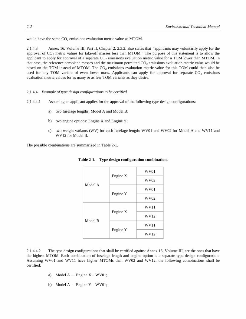


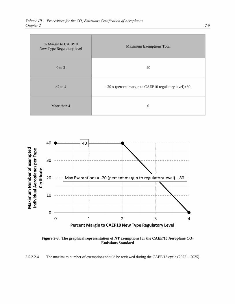


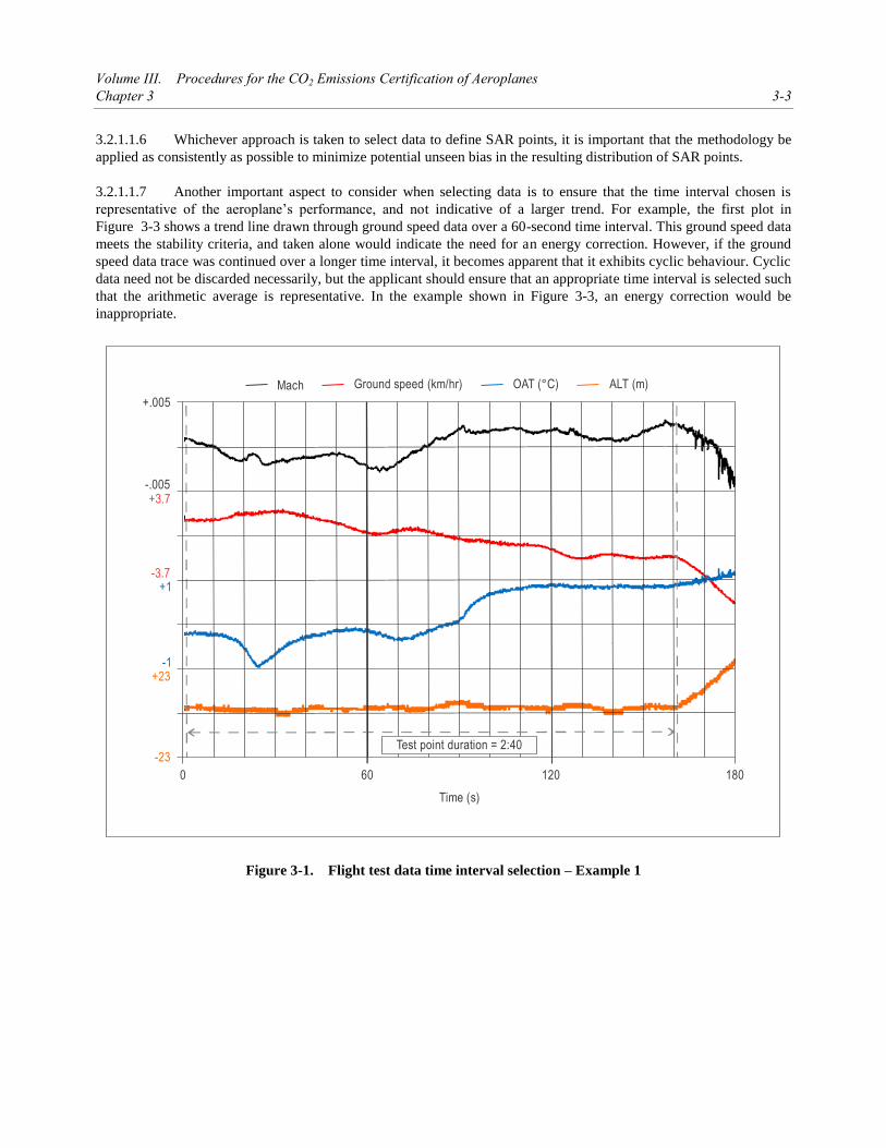

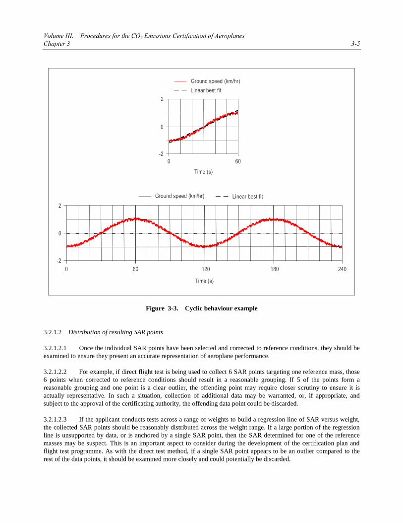

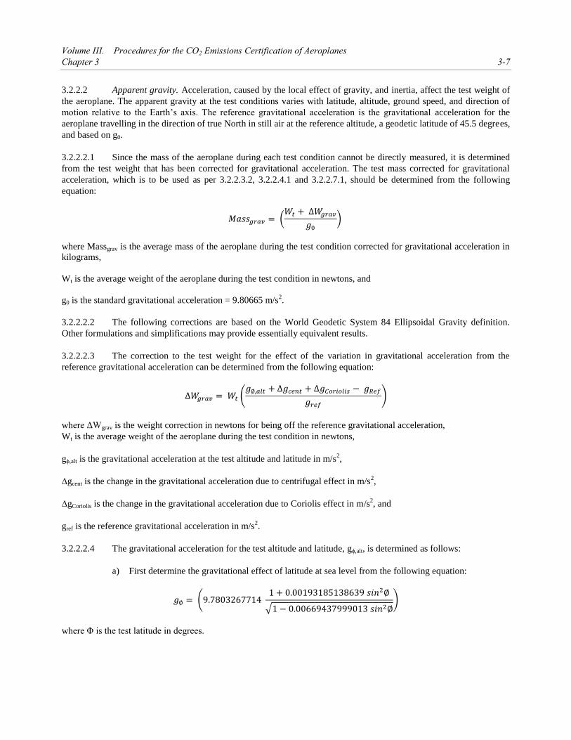


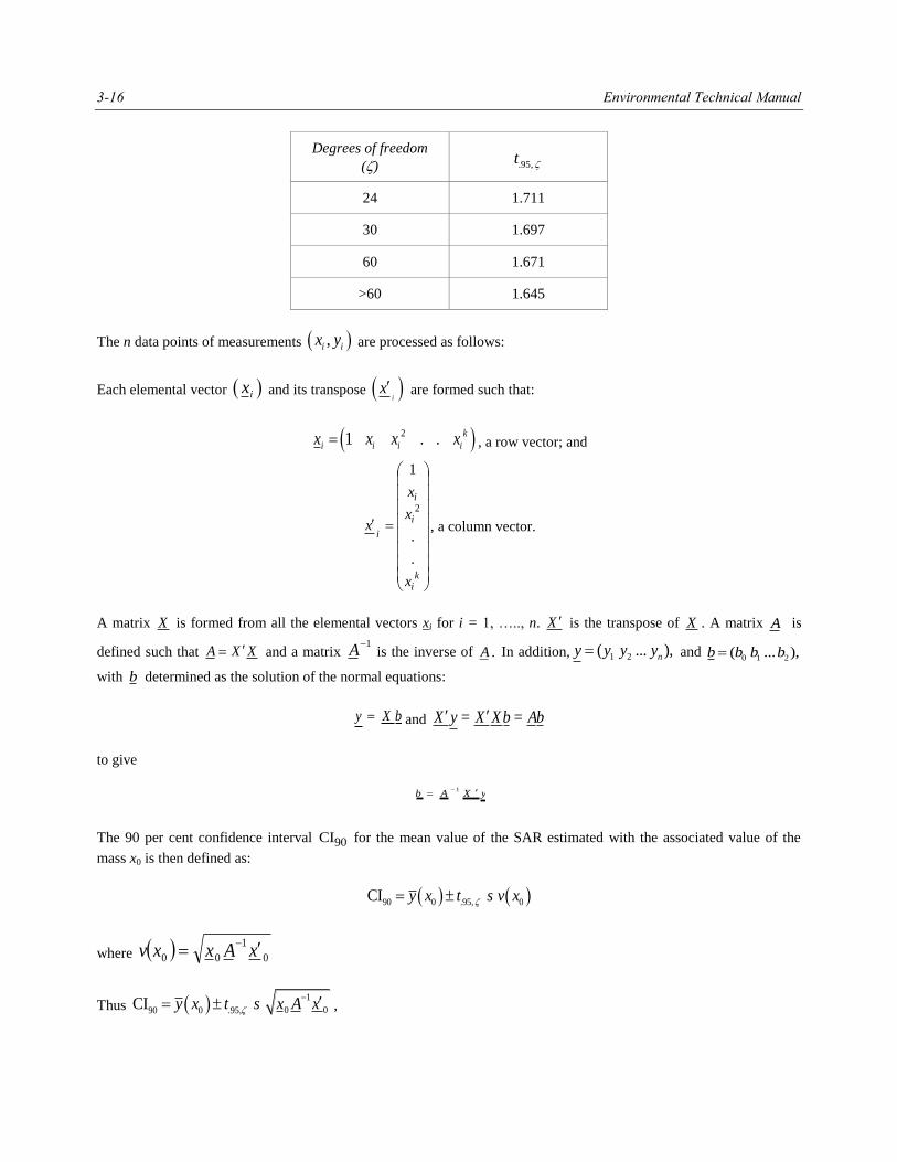


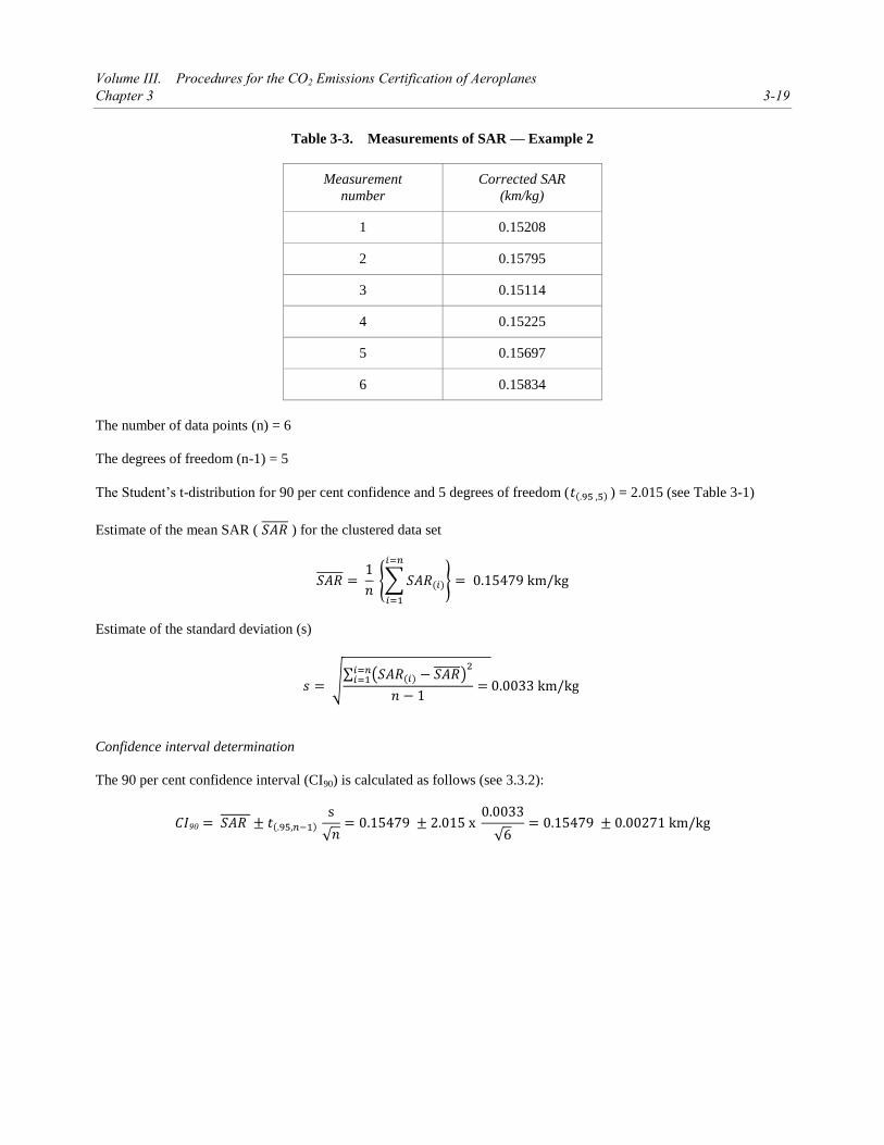


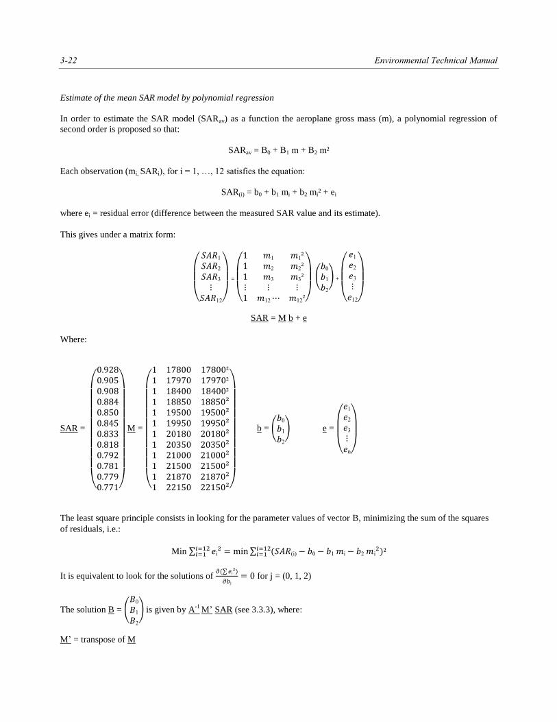


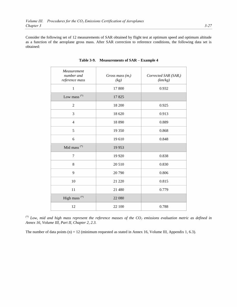


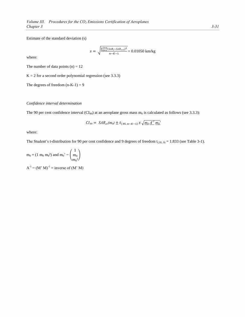


![Doc 10004 - International Civil Aviation Organization · %m a * ' $ % 9 ? $a 9)] 0/ ... ˙a (doc 9859 ) ' /)a +) * j˝ –](https://static.documents.pub/doc/80x56/5b662bfc7f8b9a2f5c8c9650/doc-10004-international-civil-aviation-organization-m-a-9-a-9.jpg)

