Electronic Supplementary Material for Shifts and disruptions in resource-use trait syndromes during the evolution of herbaceous crops by Milla R*, Morente-López J, Alonso-Rodrigo JM, Martín-Robles N, Chapin III FS *To whom correspondence should be addressed. E-mail: [email protected]This file includes: 1) Full Materials and Methods 2) Supplementary Tables S1 to S8: Table S1: Botanical name, domestication status, and seed origin information of each accession of the extensive set of 30 crop-wild ancestor pairs used in this study. Table S2: Botanical name, domestication status, and seed origin information of each accession of the intensive set of six crop species that were studied in more detail. Table S3: PCA loadings of each log-scaled individual trait on the first PCA axes named as SIZE, LIGHT COMP, LEAF ECON, and ROOT ECON. Table S4: Spearman correlation coefficients matrices. Table S5. PERMANOVA results for treatment effects and interactions (Domestication Status, Crop identity, and Dom.Status * Crop id.) on traits and PCA eigenvalues of the extensive 30 species dataset. 1
Transcript
Electronic Supplementary Material for
Shifts and disruptions in resource-use trait syndromes during the evolution of herbaceous crops
by Milla R*, Morente-López J, Alonso-Rodrigo JM, Martín-Robles N, Chapin III FS
*To whom correspondence should be addressed. E-mail: [email protected]
This file includes:
1) Full Materials and Methods
2) Supplementary Tables S1 to S8:
Table S1: Botanical name, domestication status, and seed origin information of each accession of the extensive set of 30 crop-wild ancestor pairs used in this study.
Table S2: Botanical name, domestication status, and seed origin information of each accession of the intensive set of six crop species that were studied in more detail.
Table S3: PCA loadings of each log-scaled individual trait on the first PCA axes named as SIZE, LIGHT COMP, LEAF ECON, and ROOT ECON.
Table S5. PERMANOVA results for treatment effects and interactions (Domestication Status, Crop identity, and Dom.Status * Crop id.) on traits and PCA eigenvalues of the extensive 30 species dataset.
Table S6. PERMANOVA results for treatment effects and interactions (Domestication Status, Crop identity, and Dom.Status * Crop id.) on traits and PCA eigenvalues of part of the intensive dataset where six species where investigated in more detail.
Table S7. PERMANOVA results for treatment effects and interactions (Domestication Status, Crop identity, and Dom.Status * Crop id.) on traits and PCA eigenvalues of part of the intensive dataset where six species where investigated in more detail.
Table S8: Log-likelihood ratio tests for comparing correlation matrices of Traits vs those of Trait variation during crop evolution (“Traits” vs “∆C-WTrait”); and for comparing Trait evolution during early
1
domestication vs Trait evolution during later improvement (“∆LR-WITrait” vs “∆IM-LRTrait”).
3) Supplementary Figures S1 to S6:
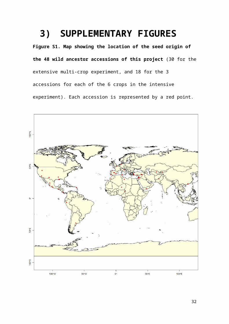
Figure S1. Map showing the location of the seed origin of the 48 wild ancestor accessions of this project
Figure S2: Phylogenetic diversity of the crop species of this project.
Figure S3: Bisector plots of the score of each crop on the 4 PCA axes associated with trait variation in Size (A), Competitive ability for light (B), Leaf economics (C) and Root economics (D).
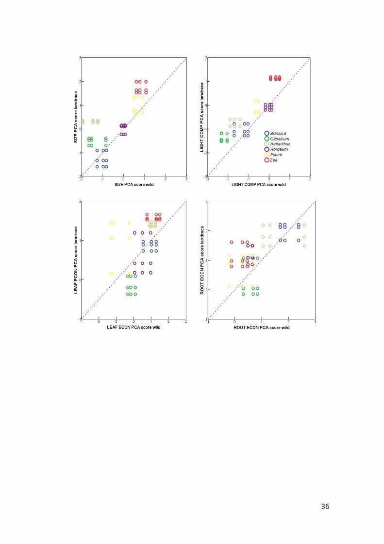
Figure S4: Bisector plots of PCA scores of three wild (x-axis) and three landrace (y-axis) accessions of each of the six crop species investigated in more detail.
Figure S5: Bisector plots of PCA scores of three landrace (x-axis) and three improved (y-axis) accessions of each of the six crop species investigated in more detail.
Figure S6: Frequency distribution of Specific Leaf Area in the Glopnet database vs that of wild accessions of the current paper.
4) Supplementary SEM analyses
5) Supplementary phenotypic integration analyses
6) References cited in Supplementary Material
Other Supplementary Material for this manuscript includes the following:1) Supplementary Data (milla_etal_Supplementary_Data_S1.xls):
S.D. 1a: Extensive database: Trait data for a crop and a wild ancestor accession of each of 30 crop species.
S.D. 1b: Intensive database: Trait data for three wild, three landrace, and three improved cultivar accessions of each of six crop species.
2
1) FULL MATERIALS AND METHODS
Study system, and collection and selection of seed material
We studied the process of domestication in 30 herbaceous crop species important to human food supply (see Table 1 in the main body of the paper for a species list). These include a diverse array of phylogenetically and functionally different crops with distinct domestication geographies and histories (Figs S1 and S2, [1]). In an extensive experiment we compared two accessions for each of the 30 crop species: a modern domesticated crop cultivar and a related wild species known to be its most likely wild ancestor. In a second intensive experiment we compared nine accessions for six of those thirty crops. Three of those nine accessions were geographically diverse provenances of the putative wild ancestor. Three others were landraces, as representatives of an initial stage of domestication. The final three were commercial varieties that have undergone modern breeding improvement programs. The accessions of the intensive experiment were selected to include a broad range of geographical wild provenances (wilds), of ethnographically diverse landraces (landraces), and of varietal diversity for modern crops (improved). The six crop species selected for the intensive experiment were maize, barley, pea, pepper, sunflower, and collard. These species were chosen for their taxonomic and functional diversity and agronomic relevance. See Table S1 for accession identifiers, seed donors, domestication status, and literature source for wild ancestor assignment of the extensive experiment, and Table S2 for the same information for the intensive experiment.
Criteria for selecting traits, experimental approach and plant measurements
We selected a set of nine plant traits to encompass four independent plant functions: competitive ability for light, leaf resource-use strategy, root resource-use strategy, and size-allometry. We adopted a soft-traits approach to select specifically measured traits [2]. Seed and whole plant dry weight were selected as proxies for whole organism and organ sizes [3]. Specific Leaf Area and Leaf Dry Matter Content were used to signify leaf resource-use strategy [4]. Specific Root Length and Fine Root Tissue Density were analogously used to signify root resource-use strategy [5]. And Absolute Growth Rate in Height of seedlings, Maximum Canopy Height, and Leaf Area were employed as proxies to competitive ability for light [6].
3
During 2011 and 2012 we conducted several common garden experiments to build the trait databases for the extensive and the intensive experiments described in the previous subsection. In 2011, approximately 20 seeds for each of 60 crop-wild paired accessions aimed for the extensive database were weighed to the nearest microgram with a microbalance (MT XP6, Mettler-Toledo Inc., Westerville, Ohio, USA), set to germinate on moist filter paper in dark-cold growth chambers and, when radicle emergence was observable, transplanted to individual 5x5x10 cm containers filled with commercial potting soil, and set in a greenhouse (Universidad Rey Juan Carlos, Móstoles-Madrid, Spain, 40o18´48´´N-3o52´57´´W, mean annual temperature: 14ºC, mean annual precipitation: 481 mm, long-term data from http://opengis.uab.es/wms/iberia/mms/index.htm). Seedlings were kept in the greenhouse for three to six weeks, depending on developmental speed of the crop species. Then, 15 individuals per accession were transplanted outdoors to free-rooting planting beds in an experimental field beside the greenhouse. Watering in the greenhouse and in the experimental fields was supplied at dawn and/or sunset through regular automatic water sprinkling and drip irrigation, respectively, and as needed to maintain plants under optimal growing conditions. All the above plant growth procedures were carried out sequentially through the season, matching the most appropriate time of the year for the performance of each crop species. The two accessions of each crop species were always sown concurrently and at the same spatial location within the greenhouse and planting bed, and were transplanted to the planting bed at the same time.
The plants grown in 2011 were used to obtain 5-20 (median = 15) replicate scores, for each accession of the extensive experiment, of the following traits: 1) Seed Size (mg), as described above; 2) Leaf Size, measured as one-sided projected surface area (LA, cm2); 3) Specific Leaf Area (cm2 g), measured as leaf surface area per oven-dried mass of leaf laminas; 4) Leaf Dry Matter Content (g g-1), as the oven-dried leaf mass divided per mass of the leaf taken to full turgidity; 5) Seedling Absolute Height Growth Rate (cm d-1), as the early rate of increase in height at the seedling stage; and 6) Canopy Height (cm), measured, before transplanting to planting beds, as the distance from soil surface to the highest node of the main shoot. Protocols for trait measurement described below follow [3]. Both accessions of a given crop were always measured concurrently at the same spatial location, even if timing of measurements was variable among crop species (e.g. number of days between initial and final height measurement below), depending on species phenology and developmental rates. After full extension of the first pair of true leaves, plant height was measured to the nearest mm. Plant height was measured again before transplanting. One representative fully mature but non senescent leaf was harvested from each of 10-15 individuals per accession. Leaves were then scanned at 400 d.p.i. using a large A3 flatbed scanner for large leaves (e.g. Beta vulgaris, WinRHIZO ProLA2400 unit, Regent Instruments Inc., Quebec, Canada). After scanning, a 1-5 cm2 piece of the lamina was cut avoiding major veins, and placed on top of a soaked piece of germination paper overnight at 4 ºC to reach full hydration. The remainder of the leaf lamina was oven-dried at 70 ºC. The following day, the 1-5 cm2
piece was weighed to the nearest microgram (MT XP6, Mettler-Toledo Inc., Westerville, Ohio, USA), oven-dried, and re-weighed. After three days at 70 ºC, all leaf material was weighed to obtain dry mass. Scanned leaves were processed with ImageJ software (http://rsb.info.nih.gov/ij) to obtain leaf area.
In 2012 we conducted an additional experiment, aimed to contribute all data for the intensive database, plus root and plant dry mass data for the extensive database. Seed weighing and germination procedures were carried out as in 2011, but germinating seeds were set into special containers appropriately built to characterize the root system. To this end, we used Root Trainers Jumbo containers that provide extra large container depth (Spencer Lemaire Ltd., Canada). Root Trainers are curly in the inside. We thus stuffed plastic cylinders inside Root Trainers to avoid root guiding through the curls of the containers, and also gain extra container depth. Containers built this way were 42 cm in depth and 8 cm in diameter. Containers were filled with commercial 100% sand substrate, aimed to facilitate the complete and integral recovery of the root system at harvest time. Plant were grown in those containers until inspection of the lower end of the containers spotted root tips for at least 3-4 plants per accession. At that time (ranging from 3 to 6 weeks since sowing date), all accessions of a given crop were harvested. Watering regime and greenhouse growth conditions were as described above for 2011, but containers were fertilized twice a week with complete nutrient solution to allow regular development in the sandy substrate.
The plants grown in 2012 were used to obtain 5-15 (median = 11) replicate scores, per each accession belonging to either the extensive or the intensive database, of the following traits: 1) Total plant Dry Mass (TDM, g) of plants kept growing for the same amount of time for all accessions of a given crop species; 2) Specific Root Length (SRL, m g-1) of the whole root system; and 3) Root Tissue Density (RTD, g cm-3). To obtain measures of those traits we proceeded as follows. At harvest time, individual plants were carefully dug and roots washed of soil particles to recover the whole root system intact. Root systems were subsequently set in a water-filled glass tray (A3-size) and scanned (gray scale, 400 dpi; [7,8]) using a flat-bed scanner (WinRHIZO ProLA2400 unit, Regent Instruments Inc., Quebec, Canada) equipped with a light transparency unit. Scanned root images were converted to binary black and white with ImageJ (http://rsb.info.nih.gov/ij). Total root length and root volume were further measured using the morphological analysis of WinRhizo (WinRHIZO Pro, Regent Instruments Inc., Quebec, Canada). Finally, the above- and the below-ground biomass of each plant was oven-dried at 70ºC for three days and weighed separately. Specific Root Length (SRL, m g-1) was calculated as the ratio between the length of the root system and its dry mass. Root Tissue Density (RTD, g cm -3) was calculated by dividing root dry mass by its fresh volume, as provided by Winrhizo software. Total plant Dry Mass (TDM, g) was the sum of above- and below-ground dry mass of each plant. Additionally, but only for the accessions belonging to the intensive database, all seed size and aboveground plant traits were measured as described above for the 2011 procedures. Canopy Height was, in this case, measured just before harvesting plants.
Data analysis
Our dataset had 3.02% missing data (31 out of 1026 accession*trait scores, see Database S1 in Supplementary Material for specific trait scores missing for specific
5
accessions). Following recommended procedures we adopted a multiple imputation approach to deal with missing data [9]. We generated ten complete datasets using Bayesian imputation, as implemented in Amos 18.0 [10]. For each of the PCA, PERMANOVA, SEM or Aster procedures described below, we used each of the ten complete databases separately. Reported parameter estimates, and measures for magnitude of goodness of fit in the main body of the paper, are average scores of fitting models to those ten complete databases. Given the low amount of missing data, in no case did statistical significance or directionality of effects of any model parameter change as a function of the dataset employed.
Effects of domestication status and crop identity on traits and on groups of traits
Traits were considered separately for analyses, and also in groups of two or three according to well-known strong physiological or developmental linkages among traits. Grouping of traits for further data analysis was performed through reduction of dimensionality. Four Principal Components Analyses were run separately for each of the following four groups of log-scaled traits. First, Seed Size and Total Dry Mass data were reduced to a first PCA axis aimed to represent organ and plant size variation among individuals (SIZE hereafter). Second, Seedling Absolute Growth Rate, Plant Canopy Height, and Leaf Size were reduced to a single PCA axis aimed to synthesize competitive ability for light capture (LIGHT COMP hereafter). Third, a PCA was run on leaf economic traits using Specific Leaf Area and Leaf Dry Matter Content (LEAF ECON hereafter). The first axis of that PCA was negatively related to structural investment in leaf tissue, which commonly correlates positively with leaf longevity and negatively with carbon fixation rates and mass-based nutrient status of leaves [11]. Lastly, a fourth PCA was run on root economic traits with Specific Root Length and Density of Fine Roots as component variables (ROOT ECON hereafter). First axes of the PCA analyses above explained 64 to 82% of variance in their composing variables (see Table S3) and were thus used as summarizing proxies of each of the four plant functions considered in this paper.
To evaluate the effects of domestication status and of crop identity on log-transformed trait and PCA axes scores, we used parameter-free permutational ANOVA analyses [12](PERMANOVA hereon). A PERMANOVA approach was preferred, instead of General Linear Mixed Model procedures, because residuals of GLMs would not accommodate normality assumptions for a majority of models, even after transforming data. In short, statistical testing in PERMANOVA approaches is based on the use of permutation tests over distance matrices derived from dataset vectors and thus do not rely on GLM assumptions. PERMANOVA analyses were carried out over Euclidean distance matrices. Statistical significance testing of model parameters was done using 4999 permutations of the raw data. Several PERMANOVA analyses were run. The first set of analyses used the extensive database. Each analysis on that database included trait values or PCA scores as the dependent variable, Domestication Status (either crop or wild) as a fixed-effect predictor, and Crop Identity (crop botanical genus) and Dom. Stat. * Crop Id. interaction as random-effect predictors. Two additional rounds of analyses were run using the intensive database. In the first round for this database we
6
assessed trait changes during initial domestication. In these analyses, we removed all data from improved (IM) accessions and used only data for wilds (WI) and landraces (LR). In the second round for the intensive database we assessed trait changes during the crop improvement phase of domestication. We thus removed WI accessions from the database and kept those with either LR or IM domestication statuses. Model specifications for PERMANOVA analyses with the intensive database were identical to those described above for the extensive database. Analyses were run with PERMANOVA+ for PRIMER statistical package (PRIMER-E Ltd., Plymounth Marine Laboratory, UK).
Coordinated evolution of traits during domestication and further improvement
A) Structural Equation Modelling:
We used Structural Equation Modelling (SEM) to investigate functional links among multiple traits, and their putative coordinated evolution during domestication [13]. First, we describe the datasets we used to build the several SEMs, and the rationale for model construction. After that, we provide statistical details on the estimation of goodness of fit, and on the statistical significance of path coefficients. Finally, in Supporting Information item 5 we provide results of additional SEM analyses aimed to provide additional empirical support for the general validity of the a priori inter-trait relationship scheme depicted in Fig. 2A in the main body of the paper.
Datasets and model construction
SEMs were implemented for two separate types of data sets. First, we put together all log-scaled arithmetic mean trait and PCA scores for each accession present in both the extensive and intensive databases (“complete” dataset hereafter, n = 114 accessions). Second, we calculated, independently for the extensive and intensive databases, the magnitude of the domestication and improvement effects over log-trait and PCA scores as follows. For the extensive database, we substracted the average score of each wild (W) accession from that of its crop (C) counterpart. This evolutionary change is denoted as ∆C-WTrait throughout the paper. For the intensive database we calculated an effect of domestication and an effect of subsequent improvement, separately. The domestication effect was taken by subtracting the average score of each wild (WI) accession from that of its landrace (LR) counterpart (∆LR-WITrait, hereafter). Since the intensive database included three accessions for each domestication status per each crop species, we subtracted every possible combination of wild accession from every landrace, for each species separately. This yielded nine ∆LR-WITrait scores per crop species included in the intensive database. We proceeded in the same way to compute the improvement effect: every score of a landrace (LR) accession was subtracted from each of the three improved (IM) accessions available for each crop species (∆IM-LRTrait, hereafter).
7
The above calculations resulted in four separate datasets: 1) a “complete” dataset, n= 114 log-scaled accession average log-trait and PCA scores; 2) “∆C-WTrait” dataset, n = 30 wild-to-crop evolutionary transitions for each trait and PCA score; 3) “∆LR-WITrait” dataset, n = 54 wild-to-landrace evolutionary transitions for each trait and PCA score; 4) “∆IM-LRTrait” dataset, n = 54 landrace-to-improved evolutionary transitions for each trait and PCA score.
Based on previous knowledge and on the patterns of trait correlation that we observed in our study, we first designed an overall causal conceptual structure that identified four groups of variables in a model. Simple arrows were employed when sufficient knowledge of the direction of causality was available, whereas double-headed arrows were used if direction of causality was either unclear or could work in both ways. This structure included the following specific expectations:
1) Groups of traits affecting specific functions (e.g. capacity to compete for light, or root foraging ability), tend to co-vary tightly. For instances, Seedling Absolute Growth Rate and Canopy Height both promote above-ground competition ability and tend to be phenotypically linked [14]. There is abundant literature supporting this assumption for the other three groups of functions modelled here: leaf economics [11,15], root economics [16,17], and size [18,19].
2) Increases in size of individuals and organs tend to result in diminishing returns in terms of physiological revenue from resource capturing organs [20,21]. Therefore, we expect increases in size-related traits to co-evolve with slower leaf and root economic traits, but to promote faster vertical growth, taller canopies, larger leaves, and therefore greater competitive ability for light.
3) Duration, structural investment, and physiological performance of fine roots and leaves may, or may not, evolve in a coordinated fashion. Theoretical proposals suggest that high photosynthetic capacity and biomass renewal rates above-ground should require rapid nutrient uptake rates and short lived fine roots belowground [22,23]. However, empirical evidence is diverse [16,17,24,25].
4) Capacity to compete for light, that is, ability to shade competitors, may interact with leaf and root economics. Above ground, this might occur as a direct effect, via trade-offs between displaying large light-capturing surfaces vs smaller but physiologically more active ones [26]. But this correlation may also arise as an indirect allometric effect of increased size (see 2 above). Increased competitive ability requires increased investment in mostly heterotrophic stem and petiole tissue [14], which might incur diminishing returns from investment in leaf photosynthetic tissue and fine root water and nutrient uptake capacity. Therefore, we predict a negative relationship between
8
capacity to compete for light and fast leaf and root economics (i.e. fast photosynthesis and water and minerals uptake rates, and fast biomass renewal rates of productive tissues).
The model structure finally selected by goodness of fit estimates should 1) address the extent to which variation in the four separate suites of traits among all accessions in our database (“complete” dataset”) is consistent with previous physiological and ecological knowledge (as outlined above); and 2) account for the extent of coordinated co-evolution of traits during domestication and further improvement, as reflected in datasets “∆C-WTrait”, “∆LR-WITrait”, and “∆IM-LRTrait”.
Considering the above a priori constraints, we generated several tentative specific models, and the model that received the highest statistical support for our “complete” dataset is shown in Figure 2B. In this model, we used the first PCA axis of each functional grouping of traits, instead of raw trait scores. This accommodates our expectation number 1 above (i.e. intense within-group coupling of trait variation) and is analogous to the usage of latent variables in complete SEM structures [27]. Also, a simpler model excluding measured traits best complied with SEM rules of thumb for sample size to number of variables ratio for our dataset [27]. Computation of PCA axes is described above (subsection “Effects of domestication status and crop identity on traits and on groups of traits”). The model in Figure 2B was further fitted to the “∆C-
WTrait”, “∆LR-WITrait”, and “∆IM-LRTrait” datasets to investigate co-evolution of traits during domestication and further improvement.
Goodness of fit measures and statistical significance of path coefficients
We used parameter-free approaches for assessing goodness of fit of models to data, and to evaluate whether single path and correlation coefficients were statistically different from zero. The degree of fit between the observed and expected covariance structures was first assessed by a χ2 goodness-of-fit test. A significant goodness-of-fit test indicates that the model does not fit the data globally. Since sample size was small for one of the four SEM models (“∆C-WTrait”), we estimated the statistical significance of χ2
goodness-of-fit statistic using two independent methods, both robust to low sample sizes. First, the probability value of the obtained χ2 was obtained with MCX2 (http://pages.usherbrooke.ca/jshipley/recherche/book.htm), which yields probability estimates for the maximum likelihood χ2-statistic based on small sample sizes [13]. Second, χ2 statistical significance was computed using the Bollen and Stine bootstrap test [28], which is also robust to small samples. However, significant χ2 can result from violation of certain assumptions, whereas failure to reject a model (a non-significant χ2) may result from inadequate statistical power [29]. Therefore, we also evaluated model fit to the data by means of the Goodness of Fit Index (GFI) and the Root Mean Square Error of Approximation (RMSEA), which are often used in SEM and are insensitive to sample size [30]. Values of GFI range between 0 and 1, and values >0.9 indicate an acceptable fit of the model to the data [30]. RMSEA values <0.1 also indicate
acceptable fit between model and data [30]. Bootstrapped and MCX2 probability values yielded practically equal statistical significances, thus only bootstrapped p-values are shown in the main body of the paper for simplicity.
Standardized path and correlation coefficients were estimated using maximum likelihood. Standardized partial-regression coefficients help interpret expected changes in the dependent variable in response to a unit of change in the predictor, while controlling for shared variance of the predictor and response with other predictors [31]. We used standardized coefficients to interpret inter-trait scaling relationships. Frequency distribution of the several dependent variables in each model did not always fit to a Gaussian distribution. Therefore, statistical significance was evaluated for each single standardized path and correlation coefficient in the model through bootstrapping [10]. Standardized path or correlations coefficients < |0.05| were constrained to be zero to achieve model identification. All SEM analyses were performed using AMOS 18.0 (SPSS Inc, Chicago, USA).
B) Analysis of phenotypic integration:
Phenotypic integration levels are often assessed based on trait-to-trait correlation matrices. Indices of phenotypic integration are computed based on magnitude of the absolute value coefficients in correlation matrices, and compared among experimental subjects or populations (e.g. eigenvalue-based INT index[32,33]). However, by definition, a non-significant correlation coefficient is indistinguishable from zero, and should be considered zero in any type of further analysis of collections of correlation coefficients. Thus, the most common approach is to quantify the number of significant correlations, and the magnitude of the absolute value of correlation coefficients, separately [34–36]. This procedure precludes the emission of a single unified answer to the hypothesis being tested, because two different components, significance and magnitude, are evaluated through separate statistical tests. However, if collections of correlation coefficients are taken as a unified dataset, such collections would most frequently accommodate a bimodal distribution, with an initial peak at zero (i.e. non-significant coefficient parameters), and a later one at the median of truly significant coefficients. Bimodality hinders most common procedures of general or generalized hypothesis testing and model evaluation [37]. To address this problem, and be able to provide a unified single test of whether phenotypic integration differed between datasets, we made use of Aster models [37,38]. Aster models were developed to address the typically bimodal distribution of lifetime fitness data [37]. Lifetime fitness is composed of the survival of a given percentage of individuals, coupled to the fecundity of survivors. In this context, Aster models account for the dependence of fitness components expressed later in ontogeny (e.g. fecundity) on processes expressed earlier (e.g. survival) [37]. This is achieved through the use of forest graph exponential family of canonical models that combine generalized linear modelling with survivorship analysis in a single statistical test [38]. We made use of Aster models here to analyze the bimodal distributions of our correlation-coefficient datasets. We dissected our correlation dataset in two “life history” components: (1) whether a correlation was statistically different from zero (analog to survivorship) and (2), if non-zero, absolute
10
magnitude of the correlation coefficient (analogous to fecundity). Statistical significance was assumed to accommodate a Bernoulli distribution, and magnitude of coefficients to follow a zero-truncated Poisson distribution.
We generated an Aster model where magnitude of correlation coefficients, conditional on prior statistical significance of coefficients, was used as the dependent variable. “Dataset” was the independent fixed effect factor, which had four levels: “complete”, “∆C-WTrait”, “∆LR-WITrait”, and “∆IM-LRTrait”(see SEM procedures above for datasets nomenclature). Significance of the “Dataset” factor was tested through comparison of our model to a reduced model where “Dataset” was not included as a predictor. This comparison was carried out through log-likelihood ratio tests [37]. If “Dataset” was found to exert a significant effect over the magnitude of correlation coefficients, then multiple paired comparisons among the four levels of “Dataset” were carried out. Those multiple comparisons were also carried out through log-likelihood ratio tests. Aster models and log-likelihood ratio tests were run using the aster and anova.aster functions, respectively, of the Aster package [37,38] available for the R platform [39]. Detailed information and resources on the mathematical basis and usage of Aster models is available at http://www.stat.umn.edu/geyer/aster/.
bank of the Leibniz Institute of Plant Genetics and Crop Plant Research, Germany;
NPGS: National Plant Germplasm System-USDA, U.S.A.; CRF: Centro Nacional de
Recursos Fitogenéticos-INIA, Spain; ICARDA: International Center for Agricultural
Research in Dry Areas-FAO, Syria; CGN: Center for Genetic Resources, The
Netherlands; UPV: Seedbank of the Polythecnic University of Valencia, Spain; CIRAD:
Centre de Coopération Internationale en Recherche Agronomique pour le
Devélopemment, France; IRRI: International Rice Research Institute; JIC: John Innes
Center; * commercial company). Accession identifier refers to the code assigned by
each seed donor excepting the commercial companies (N.A., not applicable). Accession
country refers to the country where the seeds were collected, if applicable. Ref:
reference source for wild ancestor assignment (Ref list is provided as a footnote below
the Table).
12
13
Botanical name Dom. statusAccesion identifier Seed donor
Accesion country Ref.
Avena sativa C BGE024681 CRF Spain 1Avena sterilis W IG 100379 IFMI 3096ICARDA Turkey 1Beta vulgaris C N.A. Clause* commercial 1Beta vulgaris W 1582 IPK Italy 1Brassica oleracea C N.A. Rocalba* commercial 2Brassica oleracea W CGN18947 CGN Germany 2Capsicum anuum C N.A. Mascarell* commercial 2Capsicum anuum W PI631137 NPGS Guatemala 2Capsicum bacattum C CGN23297 CGN Peru 2Capsicum bacattum W CGN23278 CGN Argentina 2Cicer arietinum C BGE024684 CRF commercial 2Cicer reticulatum W IG72945 ILWC116 ICARDA Turkey 2Cichorium endibia C N.A. Rocalba* commercial 3Cichorium intybus W BGE032596 CRF Spain 3Cynara cardunculus C N.A. Rocalba* Spain 4Cynara cardunculus W ES-01-14-0256 Semillas Silvestres*Spain 4Eruca sativa C N.A. Rocalba* commercial 5Eruca sativa W ERU 115 IPK Pakistan 5Glycine max C N.A. Biográ* commercial 6Glycine soja W 1039 IPK Russia 6Gossypium hirsutum C BGE006434 CRF USA 2Gossypium hirsutum W BG 6050 CIRAD France 2Helianthus annuus C HEL 226 IPK USA 2Helianthus annuus W PI413093 NPGS USA 2Hordeum vulgare C BGE000214 CRF commercial 2Hordeum spontaneum W BGE025385 CRF Morocco 2Lathyrus sativus C BGE014724 CRF Spain 7Lathyrus cicera W BGE019570 CRF Spain 7Lens culinaris C BGE024692 CRF commercial 2Lens orientalis W IG 72642 IFWL 119 ICARDA Syria 2Lupinus luteus C LO4500 CRF commercial 8Lupinus luteus W LO4579 CRF Portugal 8Solanum lycopersicum C N.A. Clause* commercial 2Solanum pimpinellifoliumW LA1383 NPGS Peru 2Medicago lupulina C N.A. Intersemillas* commercial 9Medicago lupulina W IG 58734 IFMA 6092 ICARDA Turkey 9Oryza sativa C N.A. Calasparra* commercial 10Oryza nivara W IRGC 104969 IRRI China 10Pennisetum glaucum C PI586660 NPGS Burkina Fasso 11Pennisetum glaucum W PI537068 NPGS Niger 11Pisum sativum C 2600 JIC commercial 2Pisum humile W 1794 JIC Israel 2Secale cereale C BGE010915 CRF commercial 2Secale ancestrale W PI618666 NPGS Turkey 2Sesamum indicum C N.A. Rocalba* commercial 12Sesamum indicum W 17 IPK Yemem 12Sorghum sudanense C N.A. Rocalba* commercial 2Sorghum bicolor W PI524718 NPGS Sudan 2Spinacea oleracea C N.A. Rocalba* commercial 13Spinacea turkestanica W CGN9546 CGN Uzbekistan 13Trifolium repens C N.A. Intersemillas* commercial 14Trifolium repens W CGN22513 CGN Kyrgyzstan 14Triticum durum C BGE020911 CRF commercial 2Triticum diccocoides W 352322 NPGS Lebanon 2Vicia faba C N.A. Rocalba* commercial 1Vicia narbonensis W IG 111590 IFVI 5266 ICARDA Tunisia 1Vigna unguiculata C PI599213 NPGS commercial 15Vigna unguiculata W PI447516 NPGS Nigeria 15Zea mays C Ames26252 NPGS Brazil 16Zea mays W PI566674 NPGS Mexico 16
Footnote: 1. Hancock, JF. 2004. Plant Evolution and the origin of crop species. CABI
Publishing, NY, USA. 2. Sauer, JD. 1993. Historical geography of crop plants. A
select roster. CRC Press. Boca Raton, USA. 3. Kiær LP, et al. 2009. Genetic Resources and
Crop Evolution, 56, 405-419. 4. Sonnante G, Pignone D, and Hammer K. 2007.
Annals of Botany 100: 1095–1100. 5. Pignone D, and Gómez-Campo C. 2011. Eruca. In
Wild Crop Relatives: Genomic and Breeding Resources, Oilseeds (Kole C, ed). Pp. 149-160.
272-288. 7. Sarker A, El Moncim A, and Maxted N. 2001. Grasspea and chicklings. In
Plant Genetic Resources of Legumes in the Mediterranean. Maxted and Bennett eds. Pp.
159-180.Kluwer Acad. Publishers, Dordrech, The Netherlands. 8. Wolko B et al. 2011.
Lupins. In Wild Crop Relatives: Genomic and Breeding Resources, Legume Crops and
Forages (Kole C, ed). Pp. 153-206. Springer-Verlag, Berlin. 9. A. Chandra, S. Verma, K.C.
Pandey. 2011. Biochemical Systematics and Ecology 39: 711-717. 10. Yamanaka S et al.
2003. Genetic Resources and Crop Evolution 50: 529-538. 11. Lewis LR. 2010. The
Professional Geographer 62: 377–395. 12. Fuller, DQ. 2003. Asian Agri-History 7(2),
127–137. 13. Andersen SB and Torp AM. 2011. Spinacea. in Wild Crop Relatives:
Genomic and Breeding Resources, Vegetables. (Kole C, ed). Pp. 273-276. Springer-Verlag,
Berlin. 14. Frame J, Newbould P. 1986. Advances in Agronomy 40: 1-88. 15.
Norihiko Tomooka, Akito Kaga, Takehisa Isemura, and Duncan Vaughan. 2011. Vigna. In
Wild Crop Relatives: Genomic and Breeding Resources, Legume Crops and Forages (Kole
C, ed). Pp. 291-311. Springer-Verlag, Berlin. 16. Wilkes G. 2007. Maydica 52:49-60
14
Table S2: Botanical name, domestication status, and seed origin information of
each accession of the intensive set of six crop species that were studied in more
detail. Domestication status (IM: improved; LR: landrace; WI: wild). Accessions
identifiers and countries as in Table S1. Seeds donors names as in Table S1, but
CIMMYT (Centro Internacional de Mejoramiento de Maiz y Trigo, Mexico), and CITA
(Centro de Investigación Agraria de Aragón, Spain).
15
16
Botanical name Dom. statusAccesion identifier Seed donor
Accesion country
Hordeum spontaneum WI BGE025385 CRF MoroccoHordeum spontaneum WI PI 282671 NPGS AsiaHordeum spontaneum WI PI 662181 NPGS TurkeyHordeum vulgare LR clho1246 NPGS USAHordeum vulgare LR PI 51209 NPGS IsraelHordeum vulgare LR PI 467371 NPGS FranceHordeum vulgare IM N.A. Batllé* commercialHordeum vulgare IM N.A. Batllé* commercialHordeum vulgare IM N.A. Batllé* commercialCapsicum anuum WI CGN22774 CGN GuatemalaCapsicum anuum WI CGN22865 CGN USACapsicum anuum WI CGN23200 CGN Costa RicaCapsicum anuum LR CGN21530 CGN NigeriaCapsicum anuum LR CGN24354 CGN MexicoCapsicum anuum LR CGN16901 CGN ChinaCapsicum anuum IM N.A. Fitó* commercialCapsicum anuum IM N.A. Fitó* commercialCapsicum anuum IM N.A. Fitó* commercialZea mays WI 27460 CIMMYT MexicoZea mays WI 27478 CIMMYT MexicoZea mays WI 27545 CIMMYT MexicoZea mays LR 2216 CIMMYT MexicoZea mays LR 2536 CIMMYT MexicoZea mays LR 10435 CIMMYT MexicoZea mays IM N.A. Fitó* commercialZea mays IM N.A. Fitó* commercialZea mays IM N.A. Fitó* commercialHelianthus annuus WI PI 468435 NPGS USAHelianthus annuus WI PI 435500 NPGS USAHelianthus annuus WI PI 435608 NPGS USAHelianthus annuus LR PI 496266 NPGS ChinaHelianthus annuus LR PI 526256 NPGS ZimbabweHelianthus annuus LR PI 600719 NPGS USAHelianthus annuus IM N.A. Fitó* commercialHelianthus annuus IM N.A. Fitó* commercialHelianthus annuus IM N.A. Rocalba* commercialBrassica oleracea WI CGN18947 CGN GermanyBrassica oleracea WI CGN06903 CGN FranceBrassica oleracea WI 9804 UPM SpainBrassica oleracea LR CGN14079 CGN BelgiumBrassica oleracea LR CGN18467 CGN TurkeyBrassica oleracea LR BGHZ.1148 CITA SpainBrassica oleracea IM N.A. Fitó* commercialBrassica oleracea IM N.A. Batllé* commercialBrassica oleracea IM CGN18467 CGN commercialPisum humile WI 1794 JIC IsraelPisum humile WI JI 3239 JIC SyriaPisum humile WI W6 2044 NPGS TurkeyPisum sativum LR 960 JIC TurkeyPisum sativum LR 1033 JIC IndiaPisum sativum LR 1281 JIC EthiopiaPisum sativum IM N.A. Fitó* commercialPisum sativum IM N.A. Fitó* commercialPisum sativum IM N.A. Fitó* commercial
Table S3: PCA loadings of each log-scaled individual trait on the first PCA axes named as SIZE, LIGHT COMP, LEAF ECON, and ROOT ECON. % Variation accounted for by each first axis: SIZE = 77%; LIGHT COMP = 64%; LEAF ECON = 82%; and ROOT ECON = 80%.
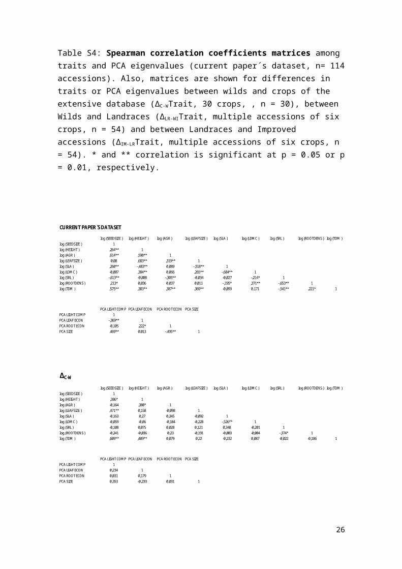
Table S4: Spearman correlation coefficients matrices among traits and PCA eigenvalues (current paper´s dataset, n= 114 accessions). Also, matrices are shown for differences in traits or PCA eigenvalues between wilds and crops of the extensive database (∆C-WTrait, 30 crops, , n = 30), between Wilds and Landraces (∆LR-WITrait, multiple accessions of six crops, n = 54) and between Landraces and Improved accessions (∆IM-LRTrait, multiple accessions of six crops, n = 54). * and ** correlation is significant at p = 0.05 or p = 0.01, respectively.
Table S5. PERMANOVA results for treatment effects and interactions (Domestication Status, Crop identity, and Dom. Status * Crop id.) on traits and PCA eigenvalues of the extensive 30 species dataset. Domestication Status has two levels (Wild and Crop). Results in Fig. 1A in the main body of the paper refer to statistics in this table. Values of P below 0.05 are shown in boldface. See Supplementary Materials and Methods for details on analyses.
20
HEIGHT AGR LEAF SIZESource of variation df MS Pseudo-F P Source of variation df MS Pseudo-F P Source of variation df MS Pseudo-F P
PCA LIGHT COMP PCA LEAF ECON PCA ROOT ECON PCA SIZESource of variation df MS Pseudo-F P Source of variation df MS Pseudo-F P Source of variation df MS Pseudo-F P Source of variation df MS Pseudo-F P
Table S6. PERMANOVA results for treatment effects and interactions (Domestication Status, Crop identity, and Dom.Status * Crop id.) on traits and PCA eigenvalues of part of the intensive dataset where six species where investigated in more detail. Here, Domestication Status has two levels, selected to characterize the early domestication effect (Wild and Landrace). Results in Fig. 1B in the main body of the paper refer to statistics in this table. Values of P below 0.05 are shown in boldface. See Supplementary Materials and Methods for details on analyses.
Table S7. PERMANOVA results for treatment effects and interactions (Domestication Status, Crop identity, and Dom.Status * Crop id.) on traits and PCA eigenvalues of part of the intensive dataset where six species where investigated in more detail. Here, Domestication Status has two levels, selected to characterize the later improvement domestication effect (Landrace and Improved). Results in Fig. 1C in the main body of the paper refer to statistics in this table. Values of P below 0.05 are shown in boldface. See Supplementary Materials and Methods for details on analyses.
CROP ID 5 48,1810 521,41 0,0002 CROP ID 5 55,9010 179,83 0,0002 CROP ID 5 34,7950 119,28 0,0002 CROP ID 5 59,8940 536,43 0,0002
DOMEST
CROP ID5 0,3576 3,8696 0,0024 DOMEST
CROP ID5 1,0202 3,2817 0,0082 DOMEST
CROP ID5 0,7922 2,7159 0,0198 DOMEST
CROP ID5 0,3125 2,7988 0,0176
Table S8: Log-likelihood ratio tests for comparing correlation matrices of Traits vs
those of Trait variation during crop evolution (“Traits” vs “∆C-WTrait”); and for comparing Trait evolution during early domestication vs Trait evolution during later improvement (“∆LR-WITrait” vs “∆IM-LRTrait”). Models under comparison are Aster models (see Materials and Methods in Supplementary Material). Change in deviance is twice the log likelihood ratio. A significant change in deviance indicates improvement of the previous model following the addition of Dataset as a predictor. Datasets codes for correlation coefficients belonging to “Traits”, “∆C-WTrait”, “∆IM-LRTrait”, or “∆LR-
WITrait” matrices. Null is a model including no predictor to provide a baseline against which to compare the effect of adding Dataset in the Full model.
General validity of the inter-trait relationships depicted in Figure 2 of the main body of the paper
We based our approach to the analysis of coordinated evolution among traits with domestication on the conceptual model of among species inter-trait relationships that is described above and supported by literature and fit to our dataset (Figure 2 of the main body of the paper).
We tested the general validity of our general model making use of the only dataset that we found in the literature that was suitable for a direct, independent, validation of our model. This dataset was taken from Laughlin et al. Functional Ecology 24: 493–501. In that paper Laughlin and colleagues make use of a 133 herbaceous species dataset to test predictions of Leaf-Height-Seed (LHS) plant strategy scheme. Data on all our traits, except plant dry mass and density of fine roots, were available for the 133 herbaceous species. We processed this database using the same procedures as with our datasets. Data were log-scaled. Dimensionality was reduced through PCA for light competition and leaf economics traits (not for plant size and root economics, for which data were only available for one trait). Then, SEM fitting was performed as for SEM models in the main body of our paper. Results of model fit and parameter estimates are shown below. Model fit was very high, and this model closely resembles the pivotal structural lines of our model (Figure 2B). Size negatively impacts root economics, and increases light competitive ability. Leaf and root economics co-vary positively. However, the trade-off between light competitive ability and leaf economics does not receive support here. Given the differences between datasets in species and parameters measured, the resemblance between the two models is remarkable and indicates that the underlying model structure has broad applicability among species.
30
We further tested the soundness of our general model by including only accessions of our dataset that qualified as wilds, using the same procedures as with the complete dataset of wild species, landraces, and crops. Technical details on model fit followed the procedures described for SEM analyses in the main body of the paper and in Supplementary Full Materials and Methods. Inter-trait relationships among traits remained similar in magnitude, directionality and statistical significance to those depicted in the complete model using all accessions (Fig. 2). This reinforces the validity of that model, and its general insensitivity to the inclusion/exclusion of non-wild accessions. Overall model fit, in this case, was lower than for the complete dataset.
31
LC ε
LIGHT COMPPCA
SRLLEAF ECONPCA
Seed Size
RE ε
-.10n.s.
-.19*
.38** -.38**
N = 133. Bootst. Pχ2 = .61GFI = .99 RMSEA <.00
(.86) (.85). 21*LE ε(.99)
LC ε
LIGHT COMPPCA
ROOT ECONPCA
LEAF ECONPCA
SIZEPCA
RE ε
-.18n.s..49**
-.52**
-.50**
N = 48. Bootst. Pχ2 = .02GFI = .99 RMSEA = .34
(.76) (.75). 23*
LE ε(.97)
5) SUPPLEMENTARY PHENOTYPIC INTEGRATION ANALYSES
Addressing the problem of the effect of heterogeneous sample sizes on the number of significant correlations
The several models and correlation matrices evaluated in this paper differ in sample size. For instance, our “general” model and corresponding correlation matrix was built out of data for 114 accessions, whereas the “∆C-WTrait”, model resulted from 30 pairs of crop species and their wild relatives, and the “∆LR-WITrait” and “∆IM-LRTrait” models were derived from a 54-accession database. The amount of paired data used to build a correlation-regression model affects several of the resulting statistics of model fit [40]. On the one hand, magnitude of slopes, or of correlation coefficients, does not consistently increase or decrease with varying sample size, but they become unstable at very low sample sizes, or when there are large variations in the ranges of focal variables [40,41]. The effects of low sample size on the magnitude of correlation coefficients are less predictable, but decreasing ranges of variation may consistently induce lower coefficients. In the Figure below we plot coefficients of variation for cultivated and wild accessions, and also for the within-crop difference between crops and wilds. Variation was of similar magnitude, or even higher, for ∆C-WTrait. Therefore, we reject the possibility that differences in the magnitude of correlation coefficients are due to contrasting degree of variability among datasets.
32
Regarding sample size and statistical significance tests of regression-correlation model parameters, tests of significance become vulnerable to type I errors as sample size increases [13]. We specifically included statistical significance as one of our components of phenotypic integration in Aster models (see Full Materials and Methods above). Thus, the differences between phenotypic integration levels among the two upper models shown in Figure 4 in the main body of the paper might arise, in part, from the effect of sample size on statistical significance of correlations.
To address this concern, we developed sets of comparisons of correlation matrices built from subsamples of equal sample size. For comparing the 114 “complete” dataset vs the 30 “∆C-WTrait”, we randomly generated fifty 30-sample sets from the 114-sample large dataset. Then, we fitted 50 Aster models to each of those 50 datasets and compared them through log-likelihood ratio tests, model-by-model, to the 30 “∆C-WTrait” dataset. 45 out of 50 log-likelihood ratio tests remained significant when sample size was forced to be equal among the datasets under comparison (see Figure below). In light of those results, we assert that the differences among “Datasets” shown in the paper are not due to contrasting sample sizes.
33
0,01 0,02 0,03 0,04 0,05 0,06 0,07 0,08 0,09 0,10
p-value
5
10
15
20
25
Freq
uenc
y
6) REFERENCES CITED IN SUPPLEMENTARY MATERIAL
1. Hancock, J. 2004 Plant evolution and the origin of crop species. Cambridge, MA: CABI Publishing.
2. Hodgson, J., Wilson, P., Hund, R., Grime, J. & Thompson, K. 1999 Allocating C-S-R plant functional types: a soft approach to a hard problem. Oikos 85, 283–294.
3. Pérez-Harguindeguy, N. et al. 2013 New handbook for standardised measurement of plant functional traits worldwide. Aust. J. Bot. 61, 167–234.
4. Wilson, P., Thompson, K. & Hodgson, J. 1999 Specific leaf area and leaf dry matter content as alternative predictors of plant strategies. New Phytol. 143, 155–162.
5. Birouste, M., Zamora-Ledezma, E., Bossard, C., Pérez-Ramos, I. M. & Roumet, C. 2013 Measurement of fine root tissue density: a comparison of three methods reveals the potential of root dry matter content. Plant Soil 374, 299–313. (doi:10.1007/s11104-013-1874-y)
6. Westoby, M., Falster, D. S., Moles, A. T., Vesk, P. a. & Wright, I. J. 2002 PLANT ECOLOGICAL STRATEGIES: Some Leading Dimensions of Variation Between Species. Annu. Rev. Ecol. Syst. 33, 125–159. (doi:10.1146/annurev.ecolsys.33.010802.150452)
7. Bouma, T. J., Nielsen, K. L. & Koutstaal, B. 2000 Sample preparation and scanning protocol for computerised analysis of root length and diameter. Plant Soil 218, 185–196.
8. Himmelbauer, M. L., Loiskandl, W. & Kastanek, F. 2004 Estimating length, average diameter and surface area of roots using two different Image analyses systems. Plant Soil 260, 111–120. (doi:10.1023/B:PLSO.0000030171.28821.55)
9. Nakagawa, S. & Freckleton, R. P. 2008 Missing inaction: the dangers of ignoring missing data. Trends Ecol. Evol. 23, 592–6. (doi:10.1016/j.tree.2008.06.014)
10. Arbuckle, J. L. 2007 Amos 18 User`s Guide. Chicago, USA.:
11. Wright, I. J. et al. 2004 The worldwide leaf economics spectrum. Nature 428, 821–7. (doi:10.1038/nature02403)
12. Anderson, M. J. & Ter Braak, C. J. F. 2003 Permutation tests for multi-factorial analysis of variance. J. Stat. Comput. Simul. 73, 85–113.
34
13. Shipley, B. 2002 Cause and correlation in Biology: A user’s guide to path analysis, structural equations and causal inference. Cambridge, UK.: Cambridge Univeristy Press.
14. Falster, D. S. & Westoby, M. 2003 Plant height and evolutionary games. Trends Ecol. Evol. 18, 337–343. (doi:10.1016/S0169-5347(03)00061-2)
15. Vasseur, F., Violle, C., Enquist, B. J., Granier, C. & Vile, D. 2012 A common genetic basis to the origin of the leaf economics spectrum and metabolic scaling allometry. Ecol. Lett. 15, 1149–1157. (doi:10.1111/j.1461-0248.2012.01839.x)
16. Tjoelker, M. G., Craine, J. M., Wedin, D., Reich, P. B. & Tilman, D. 2005 Linking leaf and root trait syndromes among 39 grassland and savannah species. New Phytol. 167, 493–508. (doi:10.1111/j.1469-8137.2005.01428.x)
17. Ryser, P. 1996 The importance of tissue density for growth and lifespan of leaves and roots: a comparison of five ecologically contrasting grasses. Funct. Ecol. 10, 717–723.
18. Jakobsson, A. & Eriksson, O. 2000 A comparative study of seed number, seed size, seedling size and recruitment in grassland plants. Oikos 88, 494–502.
19. Moles, A. T., Ackerly, D. D., Webb, C. O., Tweddle, J. C., Dickie, J. B., Pitman, A. J. & Westoby, M. 2005 Factors that shape seed mass evolution. Proc. Natl. Acad. Sci. U. S. A. 102, 10540–4. (doi:10.1073/pnas.0501473102)
20. West, G. B., Brown, J. H. & Enquist, B. J. 1997 A General Model for the Origin of Allometric Scaling Laws in Biology. Science (80-. ). 276, 122–126. (doi:10.1126/science.276.5309.122)
21. Niklas, K. J., Cobb, E. D., Niinemets, U., Reich, P. B., Sellin, A., Shipley, B. & Wright, I. J. 2007 “Diminishing returns” in the scaling of functional leaf traits across and within species groups. Proc. Natl. Acad. Sci. U. S. A. 104, 8891–6. (doi:10.1073/pnas.0701135104)
22. Grime, J. P. 2001 Plant Strategies, Vegetation Processes and Ecosystem Properties. 2nd edn. Chichester, UK: John Wiley & Sons.
23. Chapin, F. S. 1980 The mineral nutrition of wild plants. Annu. Rev. Ecol. Syst. 11, 233–260.
24. Craine, J. M., Lee, W. G., Bond, W. J., Williams, R. J. & Johnson, L. C. 2005 Environmental contraints on a global relationship among leaf and root traits of grasses. Ecology 86, 12–19.
25. Kembel, S. W. & Cahill, J. F. 2011 Independent evolution of leaf and root traits within and among temperate grassland plant communities. PLoS One 6, e19992. (doi:10.1371/journal.pone.0019992)
35
26. Lloyd, J., Bloomfield, K., Domingues, T. & Farquhar, G. 2013 Photosynthetically relevant foliar traits correlating better on a mass vs an area basis : of ecophysiological relevance or just a case of mathematical imperatives and statistical quicksand? New Phytol. 199, 311–321.
27. Grace, J. 2006 Structural Equation Modeling and Natural Systems. Cambridge, UK: Cambridge University Press.
28. Bollen, K. & Stine, R. 1992 Bootstrapping Goodness-of-Fit Measures in Structural Equation Models. Sociol. Methods Res. 21, 205–229.
29. Bentler, P. 1989 EQS structural equations program manual. Los Angeles, USA: BMDP Statistical Software.
30. Schermelleh-engel, K., Moosbrugger, H. & Müller, H. 2003 Evaluating the Fit of Structural Equation Models : Tests of Significance and Descriptive Goodness-of-Fit Measures. Methods Psychol. Res. Online 8, 23–74.
31. Grace, J. & Bollen, K. 2005 Interpreting the results from multiple regression and structural equation models. Bull. Ecol. Soc. Am. , 283–313.
32. Chreverud, J., Wagner, G. & Dow, M. 1989 Methods for the comparative analysis of variation patterns. Syst. Zool. 38, 201–213.
33. Armbruster, W. S., Pélabon, C., Bolstad, G. H. & Hansen, T. F. 2014 Integrated phenotypes : understanding trait covariation in plants and animals. Phil Trans R Soc 369, 20130245.
34. Schlichting, C. 1989 Phenotypic plasticity in Phlox. II. Plasticity of character correlations. Oecologia 78, 496–501.
35. Pigliucci, M. & Marlow, E. 2001 Differentiation for flowering time and phenotypic integration in Arabidopsis thaliana in response to season length and vernalization. Oecologia 127, 501–508.
36. Pigliucci, M. 2002 Touchy and Bushy : Phenotypic Plasticity and Integration in Response to Wind Stimulation in Arabidopsis thaliana. Int. J. Plant Sci. 163, 399–408.
37. Shaw, R. G., Geyer, C. J., Wagenius, S., Hangelbroek, H. H. & Etterson, J. R. 2008 Unifying life-history analyses for inference of fitness and population growth. Am. Nat. 172, E35–47. (doi:10.1086/588063)
38. Geyer, C. J., Wagenius, S. & Shaw, R. G. 2007 Aster models for life history analysis. Biometrika 94, 415–426. (doi:10.1093/biomet/asm030)
39. R Core Team 2013 R: A Language and Environment for Statistical Computing.
36
40. Kelley, K. & Maxwell, S. E. 2003 Sample size for multiple regression: obtaining regression coefficients that are accurate, not simply significant. Psychol. Methods 8, 305–21. (doi:10.1037/1082-989X.8.3.305)
41. Baumgartner, T. a. & Chung, H. 2001 Confidence Limits for Intraclass Reliability Coefficients. Meas. Phys. Educ. Exerc. Sci. 5, 179–188. (doi:10.1207/S15327841MPEE0503_4)