CHAPTER THREE

POWER FLOW AND SECURITY ASSESSMENT

3.1 Overview

The power flow analysis is an immensely substantial toll in the designing and planning

of the power system. The idea of the load flow problem is to obtain the voltage magnitudes

and angles for each bus (swing bus, generator bus and load bus) in the power system. The

security assessment and its types will be discussed to identify the system operating states (a

normal state, an alert state and an emergency state). To determine the problem of the

power flow analysis, the bus admittance matrix (Ybus) and equivalent π-circuit for the

transmission lines are going to obtain by using the procedures of the Newton Raphson

method. The Newton Raphson method is chosen to solve the load flow problem because

of a tremendous ingenuity to formulate the problem and an excellent ability of the

convergence for the unknown variables.

3.2 Introduction

Power flow analysis came into existence in the early 20th century. There were many

research works done on the load flow analysis. In the beginning, the main purpose of the

load flow analysis was to find the solution irrespective of time. Over the last 20 years,

efforts have been expended in the research and development on the numerical techniques

[57].

Power-flow or load-flow studies are of the great in planning and designing the future

expansion of power system as well as in determining the best operation of existing

systems. The principal information obtained from a power-flow study is the magnitude and

phase angle of the voltage at each bus and the real and reactive power flowing in each line

(flow in the line) [56].

Therefore the load flow study is an important tool involving numerical analysis applied

to a power system [58].

Where it analyzes the power systems in normal steady-state operation and it usually uses

simplified notation such as a one-line diagram and per-unit system. The power flow

problem consists of a given transmission network where all lines are represented by a Pi-

35

equivalent circuit and transformers by an ideal voltage transformer in series with an

impedance [59]. Therefore In order to perform a load flow study, full data must be

provided about the studied system, such as connection diagram, parameters of transformers

and lines, rated values of equipment, and the assumed values of real and reactive power for

each load [58].

There are different methods to determine the load flow for a particular system such as:

Gauss-Seidel, Newton-Raphson, and the Fast-Decoupled method [60].

The Newton-Raphson power flow method is going to be used in this thesis because of

exact problem formulation and very good convergence characteristic while Gauss-Seidal

power flow method is simple to understand, but this method is not recommended because

of poor convergence characteristics, where the Fast-Decoupled power flow method may

fail to converge in certain cases. So for these reasons Newton–Raphson power flow

method became more popular or widely used, where the Newton–Raphson method is

preferred over all traditional methods [59, 61].

A power system is said to operate in a normal state if all the loads in the system can be

supplied power by the existing generators without violating any operational constraints.

Operational constraints include the limits on the transmission line flows, as well as the

upper and lower limits on bus voltage magnitudes therefore Static security of a power

system addresses whether, after a disturbance, the system reaches a steady state operating

point without violating system operating constraints called ‘Security Constraints’. These

constraints ensure the power in the network is properly balanced, bus voltage magnitudes

and thermal limit of transmission lines are within the acceptable limits given, If any of the

constraint violates (system under contingency situation), the system may experience

disruption that could result in a `black-out' [1, 3] .

So the power system security can be defined as ability of the system to reach a state

within the specified secure region following a contingency (outage of one or several line

and transformer) [63].

3.3 Static Security Assessment (SSA)

Power system security has been recognized as an important aspect in planning, design

and operation stages since 1920s. Nowadays, power systems are forced to operate under

stressed operating conditions closer to their security limits. Under such fragile conditions,

36

any small disturbance could endanger system security and may lead to system collapse so

the security assessment is analysis performed to determine whether, and to what extent, a

power system is “reasonably” safe from serious interference to its operation security

assessment can be classified as static, dynamic and transient security assessment[63, 64,

65].

In this thesis a static security assessment is going to be discussed and depending on it in

this design of thesis as shown below in figure 3.1.

Figure 3.1: Types of Power System Security [66].

Static security is one of the main and important aspects of power system security

assessment, where it is ability of power system to keep at normal steady state before and

after contingency (unexpected failures) or to reach a steady state operating point without

violating in the system operating (limits of bus voltages and transmission line's thermal

limit) and continue feeding and transfer the power supply to consumers without

interruption, where violation in the system operating may be lead to the blackout or

collapse in that system [65].

The interruption or contingency in power system was considered from important causes

that leading the system to be at position of insecure mode as a result of crossing the

thermal limits of transmission line and the limits of bus voltages, where these

37

contingencies are happening because of outage of transmission line, equipment damage,

sudden change in load of system and loss of transformer, therefore any system can be

called as “secure system” or “normal system” if this system can remain in the normal

operation limits (the thermal limits of transmission line and the limits of bus voltages)

before and after contingency and the situation of this system is symbolized by digit one “1”

(binary 1), and any system can be named as “insecure system” or “emergency system”

when the normal operating limits (the limits on the transmission line flow as well as the

upper and lower limits on bus voltage magnitude) are violated, so this system is going to

be unable to withstand credible contingency in other words, Violations will be some

operational constraints where the situation of this system is symbolized by digit zero “0”

(binary 0).

The power systems provide much different kind of devices and equipment to enable the

system operators to monitor and manage the entire system in an effective manner as well

as is to keep the system with its devices and equipment in safe position (secure mode), also

the system operators is able to return the system back into a normal state (secure state) and

protection the system from the emergency state (insecure state) by taking appropriate and

urgent actions , therefore the power system security assessment can be classified into three

major functions that are carried out in an operations control centre:

Systems Monitoring:

Systems monitoring is the first step of the power system security assessment, where

system monitoring provides up-to-date measurement and information from all parts of the

system such as (line power flow, bus voltage, magnitude of the line current, output of the

generator, status of the circuit breaker and switch status information) through the telemetry

system then analyzing them in order to identify and determine the system operating state

[3, 4].

The system operating states can be broken into Normal state, Alert state, Emergency

state, Extreme Emergency state and Restorative state as shown below in figure 3.2.

38

Figure 3.2 Power System Operating States [10].

Normal state:

All equipment and devises operates naturally and in a secure position (without damages

or outages in transmission lines, transformers and other parts of system that lead the

system to be at insecure state), since there are no violation in the system operating limits

(the limits on the transmission line flow as well as the upper and lower limits on bus

voltage magnitude as described in equation (3.1) and equation (3.2) respectively).

| VK min | < | VK | < | VK max | k = 1, 2, 3……..n (3.1)

SK < Smax k= 1, 2, 3………n (3.2)

Where |VK| is the voltage magnitude at bus k, SK is the complex power (apparent power)

which is flowing at line.

39

The energy is going to reach the consumer without any interruption, if any line of the

transmission lines is tripped or any equipment of the system is damaged, but the power

system remains at secure condition as long as does not exceed the upper and lower limits

on bus voltage magnitude as well as the thermal limits on the transmission line so the

power in the network is correctly balanced as written in equation (3.3) and equation (3.4)

respectively.

∑k

n

PGK = PD + P Losses k = 1, 2, 3 ……. N (3.3)

∑k

n

QGK = QD + Q Losses k= 1, 2, 3 ……..N (3.4)

Where PGK and QGK, represent real and reactive powers of generators at bus (k), PD and

QD, are the total real and reactive load demands as well as P Losses and Q Losses are the real

and reactive losses in the transmission lines of the system network [1, 4, 5, 6].

Alert state:

In this state, the system variables are remain within limits (the limits on the transmission

line flow as well as the upper and lower limits on bus voltage magnitude), the alert state is

similar to the normal state in that all limits are not exceeding the acceptable borders of

transmission lines and voltage magnitude at all buses, but when a contingency happens, a

small disturbance can lead to violation of some security limits (future disturbance is going

to violate some thermal limits of transmission lines or upper and lower limits of voltage

magnitude), the system can be in the alert state by damage, loss and outage of any part of

operating system as well as unacceptable increasing in the system load, thus the security

level falls below a certain limit [1, 3, 5, 7, 8, 13].

Where the thermal limits are the maximum amount of electrical current that transmission

lines can bear, when the transmission lines sustain more than its thermal limits then the

transmission lines are going to damage over a specified time period due to an increase in

temperature on the transmission lines.

The changing in voltages of the system must be remained within the upper limits and the

lower limits of voltage magnitude then the electric power is going to reach the consumer

40

without any interruption and the damages in the electric system or customer facilities will

be not available, where the damages in the operating system may cause highly collapse of

system voltage as a result of blackout of some parts or entire system [67].

Where there are several main blackouts that have occurred in last half century, the first

main blackout was on November 9th 1965 in United States. And this blackout happened

because of heavy loading conditions which led to the fall of one of the electric

transmission lines, where this blackout impacted 30 million people and New York City had

lived in darkness for 13 hours [68].

The second major blackout was on July 13th 1977 in United States, and this blackout

happened because of in Con Edison System, where a thunderstorm dropped several electric

transmission lines, as a result of the dramatic increasing in the loads on transmission lines,

causing all transmission lines during 35 minutes. After 6 minutes entire system was out of

work where this blackout impacted 8 million people and they had lived in darkness and

resulted in economic losses estimated at 350 million U.S. dollars [68, 69].

The third main blackout was on July 23rd 1987 blackout in Tokyo. And this blackout

happened because of high peak demand due to massive hot weather conditions, where this

blackout impacted 2. 8 million people from residents of Tokyo [68].

The fourth main blackout was on July 2nd 1996 in United States because of short circuit

in transmission line, where this blackout impacted 2 million people [68].

The fifth major blackout was on August 14th 2003 in United States-Canada that

appeared in the Midwest and affected of the North-eastern and Midwestern United States

and southern Canada. And this blackout happened because of falling (tripping) of the

electric transmission lines due to a tree contact, where this blackout impacted 50 million

people in these countries [9, 68].

The sixth major blackout was on November 4th 2006 in Europe. And this blackout

began with 480KV transmission line falling, where this blackout impacted 15 million

people in Europe [68].

Emergency or Unsecured state:

A power system enters the emergency mode condition when operating limits (thermal

limits of transmission line as well as the upper and lower limits on bus voltage magnitude)

are violated. When the system in the emergency state, and suddenly a contingency occurs

if the operator of system did not take the immediate corrective action in due course to bring

41

the system back to the alert state, the system will cross from the emergency state to the

Extreme Emergency state or collapse of the system [3, 7, 8].

Extreme Emergency state:

The extreme emergency state is a result of an extreme disturbance or incorrect protective

action or inefficient emergency control action, where the system in this state is close to

collapse or shut down. A proper control action must be taken to rescue the system as much

as possible from occurrence of blackout and collapse (breakdown) as well as to transit the

system into a restorative state. If these protective actions do not affect, the result is total

blackout and shutdown in that system [10].

Restorative state:

Restorative state is the transition state between normal or alert and extreme emergency

states, where in this state the operator of the system will make an immediate corrective

action in due course to restore services to power system, then the system will transit to one

of the safest states [3, 10, 64].

Contingency analysis:

A contingency is a failure of any one piece of equipment, as well as that, the outage of

transformer or transmission line. The outage occurs whenever a transmission line or

transformer is removed from service for purposes of scheduled maintenance or they may

be forced by weather conditions, faults, and technical errors by operator of the system or

other contingencies where and new steady-state operating conditions are established.

Therefore operator of the system must be able to guess how the bus voltages and line flows

will be changed in the new steady state by using long and deep experience of the operator

or specific programs, which can evaluate the contingency analysis. So the contingency

analysis is used to forebode the possible systems outage and their effect [4, 13].

There are three types of contingencies:

(N-1) contingency condition: in this condition, only one of system component will fall

(transformer or transmission line).

42

(N-2) contingency condition: in this condition, two one of system component will fall.

(N-X) contingency condition: in this condition, multiple elements of system component

will fall, where x is the number of the outage components, under these types of

contingencies, operator of the system must be able to choose the corrective preventive

action, which it appropriates with that contingency condition [4, 13].

Security control:

In this condition the operating system will be at insecure mode, operator of the system

must take the corrective preventive action to bring the system back to the normal state and

to avoid collapse of the system [4, 64].

3.4 A Brief History of the Power Flow

As soon as usage of an interconnected network for transporting of electric power led to

improve the economy and the reliability, and this effect recognized very well over half a

century ago. But the ability to predict the critical information (the voltages at all buses and

flows on network components) was still the problem, for this reason the challenge started

by development a tool that would produce this critical information. This tool was called the

load-flow or the power flow, this tool came very famous and widely used by power

engineers because of its brilliant and imaginative ability to predict the voltages at all buses

and flows on network components. In the past the calculator boards were used to solve

problems of the load-flow, where these boards were a type of analogue computer. When

the modern digital computer entered, the mainframe machine architectures were developed

by IBM Corporation and the first papers on the power flow algorithms were published by

theorists. Gauss-Seidel method was the earliest algorithms to solve the power-flow

problem, but this method is not recommended because of poor convergence characteristic

with large system, because of this problem in Gauss-Seidel method, the iterative method is

called Newton, which has represented the solution of matrix equation in large system.

In the sixties, many extensions have been made in power- flow methods. In the

seventies, the Fast-Decoupled power flow method was presented. The Fast-Decoupled

43

method enhanced a speed of algorithm. Until these days, the development is still going to

get the best results in problem of power flow [70].

3.4.1 Concept of Power Flow

Power flow or load flow is the heart and one of the most important parts of power

system planning and operation, as well as that, power flow studies are an amazing starting

point for dynamic and transient stability studies.

In 1962, the concept of load flow problem was introduced by Carpentier. The main goal

of the power-flow solution is to obtain complete voltage angle and voltage magnitude

information for each bus bar connected to the network of that power system with

corresponding to specified system operating conditions, as well as that, real powers and

reactive powers at various transmission lines as shown below in figure 3.3.

Figure 3.3: Single line diagram of 5-Buses power flow.

This line diagram contains: 5 buses, 3 generators, 4 loads and 6 transmission lines. The

second bus was taken to study the power flow on it, where all currents at the second bus

44

are flowing from this bus to other buses that they connected with it. Generator is connected

to this bus and it injects real power of generator (PG) and reactive power of generator (QG).

Load is connected to this bus and it draws real power of load (P1) and reactive power of

load (Q1).

Where the second bus is connected with the first bus by the first transmission line, and it

is connected with the third bus by the third transmission line, as well as that, it is connected

with the fourth bus by the fourth transmission line. The voltage, real power and reactive

power of this bus are equal to:

Voltage (V) at second bus = voltage magnitude |V| * voltage angle (δ).

Real power at second bus (P2) = real power of generator at the second bus (PG2) – real

power of load at the second bus (PL2).

Reactive power at second bus (Q2) = reactive power of generator at the second bus (QG2)

– reactive power of load at the second bus (QL2).

Also the total real and reactive powers at the second bus are equal to:

Real power at second bus (P2) = transmitted real power at the first line (P21) +

transmitted real power at the third line (P23) + transmitted real power at the fourth line (P24)

.

Reactive power at second bus (Q2) = transmitted reactive power at the first line (Q21) +

transmitted reactive power at the third line (Q23) + transmitted reactive power at the fourth

line (Q24) .

So the real and reactive power injection at the second bus is equal to summation of the

real and reactive powers flowing out the bus. The real power balance at all buses and total

system can be expressed as:

∑i

n

PGi + ∑i

n

PDi – P losses = 0 i = 1, 2, 3……N (3.5)

PGi represent the real powers of generators at bus (i).

PDi represent the real load demands at bus (i).

P losses represent the real losses in the transmission lines of the system network. Where

the real losses (Plossess) at each transmission line can be expressed as:

P losses = | I2| * R (3.6)

R represents resistance of transmission line.

I act the current in the transmission line.

45

The reactive power balance at all buses and total system can be expressed as:

∑i

n

QGi + ∑i

n

QDi – Q losses = 0 i = 1, 2, 3……N (3.7)

QGi represents the reactive powers of generators at bus (i).

QDi represent the reactive load demands at bus (i).

Qlossess represent the real losses in the transmission lines of the system network. Where the

reactive losses (Q losses) at each transmission line can be expressed as:

Q losses = | I2| * X (3.8)

X represents series reactance of transmission line.

I act the current in the transmission line.

All transmission lines are represented by a Pi-equivalent circuit at medium length. The

load flow solves the problem of the power system in normal steady-state operating and

planning, for making the power system more easily a one-line diagram and per unit system

will be used.

The steady state power and reactive power provided by each bus in a power system are

solved by using nonlinear algebraic equations, where these equations are algebraic because

of these equations do not contain derivative functions in the formulating of these equations,

therefore there is no differential equation only algebraic equation. And these equations are

nonlinear because of these equations contain sinusoidal functions (sine & cosine).

Because of the equations of the power system are nonlinear in nature, therefore iterative

numerical techniques will be used such as: Gauss-Seidel (G-S), Newton-Raphson (N-R),

and the Fast-Decoupled method.

The Newton-Raphson (N-R) power flow method is going to use in this thesis because of

exact problem formulation and a faster convergence characteristic, while Gauss-Seidal (G-

S) load flow method is simple to understand, but this method is not recommended because

of poor convergence characteristic, where the Fast-Decoupled power flow method may fail

to converge in certain cases [57, 58, 59, 60, 61, 71].

After finding the voltages at various bus bar and real and reactive powers at all

transmission lines, the operating conditions (thermal limits of transmission lines and

voltages limits) will be assessed to prevent the system from many problems and to

guarantee that system will stay at secure position.

46

For all these reasons, the load flow study represents the backbone of the power system

[72].

3.4.2 Bus Classification

The meeting point of different components in the network of the power system knows as

the bus bar. In practical life, the bus is a conductor manufactured from aluminium or

copper.

In the power system every node or bus is associated with four essential elements and

they are: reactive power which is symbolized as (Q), real power which is symbolized as

(P), phase angle of the voltage at various buses which is symbolized as (δ) and voltage

magnitude which is symbolized as |V|. During solution of the power flow, two of these

variables are required to be solved by equations of the power flow and the rest of the

variables are specified. The buses of the power system are divided into three categories

[57, 58, 72]. They are:

Load bus

At this bus, the real power and the reactive power are specified. The voltage angle and

the voltage magnitude are unknown, so the demand is to find out the voltage angle and the

voltage magnitude through the solution of power system. Load bus is called P-Q bus

because of the load is connected to this bus [57, 58, 72].

Voltage control bus or generator bus

At this bus, the voltage magnitude and real power (active power) remain constant

through the solution of power system. So the voltage magnitude and real power (active

power) of generator bus are specified. Therefore the demand is to find out the reactive

power and the voltage angle through the solution of power system. Generator bus is called

P-V bus because of the generator is connected to this bus. The voltage magnitude of this

bus will stay constant through the solution of power system because this bus has automatic

voltage regulator (AVR) system, for that this bus is called voltage control bus [4, 57, 58,

72].

Slack bus or swing bus

47

At this bus, the voltage magnitude |V| and the voltage angle (δ) are specified, where the

reactive power and the real power are unknown. Generally, during the practical solution

the voltage magnitude |V| = 1 per unit and the voltage angle (δ) = 0 degree, the real power

in this bus refers to the total real powers generation at all buses minus the total real powers

drawn by the loads plus real losses of the transmission lines and the reactive power in this

bus refers to the total reactive powers generation at all buses minus the total reactive

powers drawn by the loads plus reactive losses of the transmission lines, therefore the slack

bus is also known as the reference bus where there is only one slack bus in the power

system design [56, 57, 58, 72]. The table 3.1 contains a summary of bus classification:

Table 3.1: Bus Classification

Types of Bus Known Variables Unknown Variables

Load or P-Q bus Real power (P), reactive

power (Q).

Voltage magnitude |V|,

voltage angle (δ).

Generator or P-V bus Real power (P), voltage

magnitude |V|.

Voltage angle (δ), reactive

power (Q).

Slack or swing bus Voltage magnitude |V|,

voltage angle (δ).

Real power (P), reactive

power (Q).

So this table will be used to solve the problem of the power flow.

3.4.3 Transmission Lines

At medium length (80 km-240 km), a transmission line can be represented by equivalent-

pi model as shown below in figure 3.4.

Figure 3.4: Equivalent π-models for a transmission line [3].

48

A transmission line is represented by an equivalent π circuit with series impedance (R +

jX) and shunt charging susceptance (B) or shunt capacitance (C) is divided evenly at each

end of equivalent-pi model, where the shunt conductance (G) was omitted because it is

fully variable, therefore the shunt conductance do not include into account.

The shunt conductance (G) locates between the ground and the conductors or between

conductors. The usage of the shunt conductance is to account the leakage current at the

insulation of cable and through the insulators of overhead lines.

The series resistance (R) and reactance (X) of transmission line in the equivalent-pi model

are responsible for losing active and reactive powers in the transmission line, where R+jX

is called impedance and it is symbolized by (Z). The losses of real power and the reactive

depend on the quantity of the current square through the transmission line as written before

in equation (3.6) and (3.8):

P losses = | I2| * R (3.6)

Q losses = | I2| * X (3.8)

In the equivalent π-models of a transmission line, the shunt charging susceptance (B) or

shunt capacitance (C) results from the difference of the potential between transmission-line

conductors, the shunt capacitance (C) exists between parallel conductors and it is omitted

when the length of a transmission line is less than 80 km.

The shunt charging susceptance equal to the shunt admittance and it is symbolized by

(Ych) in the equivalent π-models of a transmission line [48].

Each half of shunt capacitance (C/2) is injecting the reactive power into the transmission

line [26]. The effect of three parameters (R, X and C/2) can be observed at figure 3.5.

49

Figure 3.5: Effect of Transmission Line’s Parameters at π-Model.

The transmission line in figure 3.5 connects between bus (k) and bus (m), the active

power at bus (k) transmitted to bus (m) with a loss that equalled to the current square * the

series resistance, where the reactive power from the half capacitance at two sides of the

transmission line does not effect on the transmitted active power.

The reactive power at bus (k) transmitted to bus (m) with a loss that equalled to the

current square * the series reactance, each half of capacitance at two sides of the

transmission line injects a reactive power to the connected line between bus (k) and bus

(m) [56].

The transmission line has important role for transferring the electric power to the

customer without exceeding the thermal limit of the conductor at that line, the transmission

line reaches the thermal limit (current-carrying capacity) of the conductor if the electric

current heats the material of the conductor to a certain temperature usually more than 100

Celsius, if the conductor material afforded more than that temperature, the transmission

line will cut after a certain period. The thermal limit of the conductor depends on several

factors such as: speed of the wind and the ambient temperature etcetera [13].

3.4.4 Bus-Admittance Matrix

The most common approach to solve power-flow problems is to create what is known as

the bus admittance matrix and it is symbolised as (Ybus). Consider the simple power system

as shown below in figure 3.6.

50

Figure 3.6: Single line diagram of 3-Buses power system

That single line diagram consists of three buses and three transmission lines, the bus

admittance of this simple system can be calculated by using equation (3.9):

I bus = Y bus * V bus (3.9)

Obviously the bus admittance matrix gives the relationship between the voltage at each

bus and the current injection at every bus. The bus admittance matrix can be achieved by

applying Kirchhoff’s current low (KCL) at each bus of the system.

The series impedance of all transmission lines at π model are converted to admittance by

using equation (3.10):

Zij = 1/ Zij = 1/ (Rij + j Xij) = G + j Bij (3.10)

Where Zij is the series impedance of the transmission line between any two bus i and j. The

power flow solution starts with modelling the transmission line of figure 3.6 by equivalent

π-models as shown below in figure 3.7.

51

Figure 3.7: Equivalent π-models of 3-Buses Power system

The first, the second and the third transmission lines are represented by π model, where

Yij represents series admittance and Yij0 represents the first and the second half of the shunt

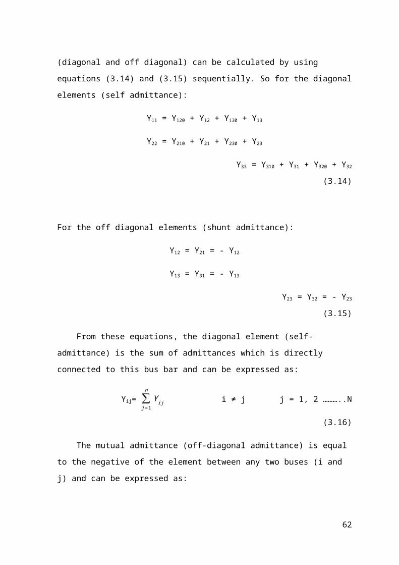
admittance. Applying Kirchhoff’s current low (KCL) at each bus of the system.

I1 = Y120 * V1 + Y12 * (V1 – V2) + Y130 * V1 + Y13 * (V1 – V3)

I2 = Y210 * V2 + Y21 * (V2 – V1) + Y230 * V2 + Y23 * (V2 – V3)

I3 = Y310 * V3 + Y31 * (V3 – V1) + Y320 * V3 + Y32 * (V3 – V2) (3.11)

Arranging these equations in a matrix form as:

[ I1I2I3]= [(Y 120+Y 12+Y 130+Y 13) −Y 12 −Y 13

−Y 21 (Y 210+Y 21+Y 230+Y 23) −Y 23

−Y 31 −Y 32 (Y 310+Y 31+Y 320+Y 32)] [V 1

V 2

V 3]

(3.12)

Also these equations can be written in another form of the matrix as:

52

[ I1I2I3]= [Y 11 Y 12 Y 13

Y 21 Y 22 Y 23

Y 31 Y 32 Y 33] [V 1

V 2

V 3] (3.13)

From equation (3.13), the bus admittance matrix consists of the diagonal elements (Y11, Y22

and Y33) and the off diagonal elements (Y12, Y21, Y13, Y31, Y23 and Y32). These elements

(diagonal and off diagonal) can be calculated by using equations (3.14) and (3.15)

sequentially. So for the diagonal elements (self admittance):

Y11 = Y120 + Y12 + Y130 + Y13

Y22 = Y210 + Y21 + Y230 + Y23

Y33 = Y310 + Y31 + Y320 + Y32 (3.14)

For the off diagonal elements (shunt admittance):

Y12 = Y21 = - Y12

Y13 = Y31 = - Y13

Y23 = Y32 = - Y23 (3.15)

From these equations, the diagonal element (self-admittance) is the sum of admittances

which is directly connected to this bus bar and can be expressed as:

Yij= ∑j=1

n

Y ij i ≠ j j = 1, 2 ………..N (3.16)

The mutual admittance (off-diagonal admittance) is equal to the negative of the element

between any two buses (i and j) and can be expressed as:

Yij = Yji = - Yij (3.17)

In general the formats of the nodal current and Y bus matrix for n-bus power system can

be written as:

Ii = ∑j=1

n

Y ij *V j j = 1, 2 …..N

53

Ii = ∑j=1

n

Y ij *V j j = 1, 2 …..N (3.18)

Ybus = [ Y 11 −Y 12

−Y 21 Y 22

⋮−Y n1

⋮−Y n2

… −Y 1n

… −Y 2n

……

⋮Y nn

] (3.19)

From all these equations, the bus admittance matrix (Ybus) has the following

characteristics:

The bus admittance matrix (Ybus) has a general complex form (G + j B).

Dimension of bus admittance matrix (Ybus) is (N * N), where N is number of buses in the

power system. If 10-buses system will be calculated, then the dimension will be (10 * 10)

Ybus matrix.

The bus admittance matrix (Ybus) is a sparse matrix, where large numbers of the elements in

the bus admittance matrix (Ybus) are zeroes because the transmission lines between any two

buses did not connect with all buses especially in large systems.

The bus admittance matrix (Ybus) is a symmetric matrix as shown in the off diagonal

elements of Ybus matrix (Yij = Yji), where the off diagonal element can be obtained as a

negative sign of the series admittance between any two buses.

Diagonal elements are the sum of admittances which is directly connected to this bus bar

(the series admittance between any two buses and the shunt admittance between the

reference and a bus in that system) [3, 56, 70, 72].

3.5 Formation of Power Flow Equations

The solution of load flow problem starts with identification the types of buses in the

power system (load bus, swing bus and generator bus), where the aim of power flow

problem are finding out the voltage magnitude and the voltage angle at various buses, as

well as that, real powers and reactive powers at various transmission lines.

The basic step in the load flow is derived from the node-voltage equation for n-bus as

shown before in equation (3.18):

54

Ii = ∑j=1

n

Y ij *V j j = 1, 2 ….N (3.18)

Where Ii is the vector of the currents injection at various buses (i), Yij is the bus

admittance matrix between any two buses and Vj is the voltage vector of different buses

where Yij and Vj can be written in polar form (magnitude and angle) as:

Yij = | Yij | θij | Yij | is the magnitude of Yij and θij is the phase angle of Yij

Vj = | Vj | δj | Vj | is the magnitude of Vj and δj is the phase angle of Vj (3.19)

The complex power injection at bus i can be written as:

Si = Pi + jQi = Vi * Ii* (3.20)

Equation (3.18) is substituted in equation (3.20) as:

Si = Pi + jQi = Vi * ¿ * Vj] * (3.21)

Vi = | Vi | δi where | Vi | is the magnitude of Vi and δi is the phase angle of Vi

By substitute the magnitude and the angle of (Vi, Vj and Yij) in equation (3.21):

Pi + jQi = | Vi | * δi * ¿ * θij * | Vj | * δj] * (3.22)

Equation (3.22) can be reformulated in polar form as:

Pi + jQi = | Vi | * ∑j=1

n

¿Y ij∨¿¿ * | Vj | * e (δi

– δj

– θij

) (3.23)

The negative signs of the angles (Vi and Vj) came from the conjugate of the current I*,

where the conjugate means same magnitude but a negative angle. Separating the real and

imaginary parts of equation (3.23) and these equations can be expressed as:

Pi = | Vi | * ∑j=1

n

¿Y ij∨¿¿ * | Vj | * cos (δi – δj – θij) (3.24)

55

Qi = | Vi | * ∑j=1

n

¿Y ij∨¿¿ * | Vj | * sin (δi – δj – θij) (3.25)

From these equations above, the power flow equations has the following characteristics:

Power flow equations represent as an algebraic equation because the power flow equations

((3.24) and (3.25)) do not contain on a differential equation in its formulation.

Power flow equations are a non linear equations equation because the power flow

equations ((3.24) and (3.25)) have sinusoidal terms (sine and cosine) and the product of

voltages.

Obviously the power flow equations ((3.24) and (3.25)) are representing a relationship

between the power injection (P and Q) at any bus (i) and the bus admittance matrix Ybus

between any two buses, as well as that, the voltage magnitude and the voltage angle of that

bus in a power system. Since the idea of power flow is to find the voltage magnitude and

the voltage angle for each bus except the swing bus because it is already given (|v| =1 per

unit and swing = 0o, so the equations of power flow will be (N-1) equations where N is a

number of buses in a power system [3, 57, 58, 60, 72].

3.5.1 Newton-Raphson (NR) method

The Newton-Raphson (NR) method is the most popular procedure to solve nonlinear

equations ((3.24) and (3.25)) of the power flow. Newton-Raphson is an iterative solution to

get the best convergence at the voltage magnitude and the voltage angle. The solution of

the power flow problem by Newton-Raphson (NR) method are based on the nonlinear

equations ((3.24) and (3.25)) and these equations are similar to the nonlinear form and can

be written as:

Y = f(x) =[ f 1 ( x )f 2 ( x )⋮f n ( x )] (3.26)

56

X = ¿ = [δ2

⋮δn

|V|2⋮

|V|n] (3.27)

Y = [PQ ] = [P2

⋮PnQ2

⋮Qn

] (3.28)

Y = f(x) = [P(x )Q(x)] = [

P2 ( x )⋮

Pn ( x )Q2 ( x )⋮

Qn ( x )] (3.29)

Where all vectors (P, Q, |V| andδ) in these equations are started from the second bus

because the first bus is usually considered as a slack (swing) bus, where the voltage

magnitude and the voltage angle of the slack bus are already given. The active power (P),

the reactive power (Q) and the voltage magnitude (|V|) are in per-unit but the angles (δ) are

in radians. The nonlinear equations ((3.24) and (3.25)) were being reformulated to be

represented later in the Taylor's series. Taylor's series expansion for Y = f(x) is written

below in equation (3.30) as:

Y= f (Xo) + df/dx |X =x0 + (X – X0) + higher-order terms (3.30)

By neglecting higher-order terms and solving for X, resulting in:

X = X0 + (df/dx |X =x0 ) -1 (Y - f (Xo)) (3.31)

But this speculation may not be very close, therefore an iterative method will be used and

it can be written as:

57

X (i + 1) = X (i) + 1 / (df/dx |X =x0 ) (i) (Y - f (X (i))) (3.32)

Equation (3.32) can be rearranged as:

X (i + 1) – X (i) = J-1 (i) (Y - f (X (i))) (3.33)

Where X (i + 1) is next updated value, X (i) is the present value where (df/dx |X =x0 ) (i) =

J (i) = [∂ f 1

∂ x1

∂ f 1

∂ x2…

∂f 2

∂ x1

∂ f 2

∂ x2…

⋮∂ f n∂ x1

⋮∂ f n∂ x2

⋮…

∂f 1

∂xn∂ f 2

∂xn⋮∂ f n∂xn

]x= x (i)

Because of component (J-1) in equation (3.33) takes much time and more complicated in

the solution therefore the equation (3.33) can be rearranged as:

J (i) ΔX (i) = ΔY (i) (3.34)

Where ΔX (i) = X (i + 1) – X (i), ΔY (i) = Y - f (X (i)) and J (i) is the Jacobian matrix. The

iterative solution is going to continue until the component (ΔY (i)) or the power mismatches

become very small and reach its convergence [57, 59, 60, 72]. For the power flow terms

(ΔY (i), ΔX (i) and J (i)) can be expressed as:

ΔY k(i)= [ ΔPk(i)ΔQk

(i)] =[ Pspceified k−¿ Pcacculatedk(i)Qspceified k−¿Qcacculatedk(i)] (3.35)

The terms (ΔP (i) and ΔQ (i)) in equation (3.35) represent the deference between the

specified (scheduled) powers and the calculated power at (i) iteration and bus (k), known

58

as the power mismatches or the power residuals, where the power mismatches mean a

noticeable difference between the real and the reactive power at that bus (k) or the

difference between the real and the reactive power at that bus (k) are more than the

specified accuracy or the acceptable tolerance [13, 57, 58, 59, 60, 72].

The Jacobian matrix (J (i)) represents a linear relation between the changes in the voltage

angle (Δδ k(i )) and the voltage magnitude (Δ|V k

(i )|) from side and the changes in the real

power (ΔPk(i)) and the reactive power (ΔQ k

(i)) from another side as written below in equation

(3.36):

[ ΔP(i)

ΔQ(i)] = [J 11(i) J 12

(i)

J 21(i) J 22

(i)] ¿ (3.36)

The Jacobian matrix (J (i)) at (i) iteration is divided into four sub matrixes and each sub

matrix can be expressed as:

J11(i )= [∂P2/∂δ2 … ∂ P2/∂δ n

⋮∂Pn/∂δ2

⋮…

⋮∂ Pn/∂δ n] (3.37)

J12(i ) = ¿ (3.38)

J21(i )= [∂Q2/∂δ2 … ∂Q2/∂δ n

⋮∂Qn/∂δ2

⋮…

⋮∂Qn/∂δ n] (3.39)

J22(i ) = ¿ (3.40)

The partial derivative in the Jacobian matrix (J (i)) is real power and the reactive power

for voltage control bus (P-V bus) and load bus (P-Q bus) in that power system with respect

to the voltage magnitude (|V|) and the voltage angle (δ) for voltage control bus (P-V bus)

and load bus (P-Q bus) in that power system because the real power and the reactive

power for voltage control bus (P-V bus) and load bus (P-Q bus) are already given but the

59

voltage magnitude (|V|) and the voltage angle (δ) for voltage control bus (P-V bus) and

load bus (P-Q bus) in that power system are unknown.

At the voltage control bus (P-V bus), the voltage magnitude (|V|) is given but the

reactive power (Q) is not known, therefore (∂Q/∂|V|) term of the voltage control bus (P-V

bus) will be deleted from the Jacobian matrix. The elements of the Jacobian matrix began

from the second bus because the first bus is a reference bus. Therefore, the numbers of the

equations to be solved in Newton Raphson method are (N – 1) equations for the real power

(P) because the real powers at the various buses are specified and (N-1-B) for the reactive

power (Q) but for B of these equations the reactive power are not known, so the total

equations for Newton Raphson method will be (2 * (N-1) – B) equations.

The power mismatches and the Jacobian elements in the equation (3.36) are used to find

the voltage error vector ¿ by using Gauss Elimination Method and the aim of the Gauss

Elimination Method is to make all elements under the main diagonal are equal to the zero,

the voltage magnitude and the voltage angle are updated after each iteration by using

equations (3.41) and (3.42) respectively:

δ(i+1) = δ(i) + Δ δ(i ) (3.41)

¿V (i+1)∨¿ = ¿V (i )∨¿ + Δ¿V (i )∨¿ (3.42)

The iteration will stop until the power mismatches (power residuals) are less than the

specified accuracy or the acceptable tolerance, then the dependent variables or the state

variables (the voltage magnitude and the voltage angle) can be calculated and the problem

of the power flow will be solved [13, 57, 58, 59, 60, 72].

3.5.2 Algorithm for Newton-Raphson method

The procedure to solve the problem of the power flow by using Newton-Raphson way is

as follows:

60

Step 1: Read the input data for power flow system (the admittance of the transmission

lines between any two buses and the transformer, as well as that, the input power

(voltage magnitude |V|, voltage angle (δ), real power (P) and the reactive power (Q))

for a specific bus (swing bus, voltage control bus (P-V bus) and the load bus (P-Q bus))

in the power flow system.

Step 2: Transformation each input of the data for power flow system into equivalent

per-unit value, where per-unit value can be defined as the ratio of the actual value to

the base value as written below in equation (3.43):

Per-unit (p.u.) value = Actual value / Base value (3.43)

The voltage-Ampere base (Sbase), the base current (Ibase) and the base impedance

(Zbase) can be determined by using equations (3.44) and (3.45) respectively:

Sbase = Vbase * Ibase (3.44)

Zbase = Vbase / Ibase

OR (3.45)

Zbase = (Vbase) 2 / Sbase

The per-unit system will be used to make the power flow system more ease and

simplicity during performing of the load flow.

Step 3: Compute the bus admittance matrix (Ybus).

Step 4: Assume an initial estimate for state vector (voltage magnitude and voltage

angle)¿ , so for all busses in power system except the swing bus and voltage control

bus (P-V bus), the voltage magnitudes of these buses will be chose as one per-unit and

for all the buses except the swing bus, the voltage angles will be chose as zero degree.

because of the voltage magnitude (|V|) and the voltage angle (δ) of the slack bus are

already given, as well as that, the voltage magnitude (|V|) of the voltage control bus (P-

61

V bus) is also given, therefore the exception consists of the swing bus and voltage

control bus (P-V bus).

Step 5: Set the iteration (i) equal to zero.

Step 6: Calculate the injected real power (P) by using equation (3.24).

Step 7: Calculate the injected reactive power (Q) by using equation (3.24).

Step 8: The estimated values (voltage magnitude (|V|) and voltage angle (δ)) are used

to calculate the Jacobian matrix (J).

Step 9: Find the voltage error vector ¿ by using equation (3.35).

Step 10: Set the tolerance value.

Step 11: Update the voltage magnitude (|V|) and voltage angle (δ) by using equations

(3.41) and (3.42) respectively.

Step 12: Check the power mismatches (ΔP and ΔQ) of the voltage control bus (P-V

bus) and load bus (P-Q bus ), if the power mismatches (ΔP and ΔQ) less than the

specified tolerance then the iterative process will be stopped, if the power mismatches

(ΔP and ΔQ) more than the specified tolerance then the iterative process will

increase(iteration = iteration + 1) and repeat this procedure procedures from step 6 until

the power mismatches (ΔP and ΔQ) of the voltage control bus (P-V bus) and load bus

(P-Q bus ) become too small and within the acceptable tolerance [57, 58, 72].

After the iteration process is stop, the final voltage magnitude (|V|) and voltage angle

(δ) are calculated therefore the problem of power flow system will be solved.

The final voltage magnitude (|V|) and voltage angle (δ) is used to find the rest

values, which are basically the real power and the reactive power at the swing bus

(slack bus), as well as that, the reactive power at the voltage control bus (P-V bus).

Therefore the key of the power flow problem is to find the voltage magnitude (|V|) and

62

voltage angle (δ) and these values will be substituted to find the rest of the unknown

values. The flow chart of Newton-Raphson procedure is shown in figure 3.8.

63

START

Read input data

Form bus admittance matrix Ybus

Assume initial bus voltage

YES yes

NO

Figure 3.8: Flowchart for Newton-Raphson algorithm.

To understand the steps of Newton-Raphson algorithm, Consider a small 3-bus system is

shown below in figure 3.9.

64

Iteration = 0

Calculate real and reactive powers

Calculate the power mismatches ΔP and ΔQ

Form Jacobian Matrix

Check ΔP and ΔQ <

tolerance

End and take the values

Calculate voltage error Δ|V| and Δδ

Update voltage magnitude |V| and voltage angle δ

Iteration = iteration + 1

Figure 3.9: 3-Buses Power- Flow system [44].

This system consists of three buses, three lines, two generators and one load. The drawn

real and the reactive powers by the load at the second bus are 400 MW and 250 MVAR.

The injected real power by the generator at the third bus is 200 MW. The first bus is

considered as the slack bus to absorb the losses of the system.

The base values are: Sbase = 100 MVA and Vbase = 138 KV. The parameters of the

transmission lines are shown in table 3.2.

Table 3.2: The parameters of the transmission lines for figure 3.9.

Number of

Transmission

line

Series

Resistance R

(p.u.)

Series

Reactance X

(p.u.)

Shunt

Charging B

(p.u.)

Shunt

Conductance G

(p.u.)

1 0.02000 0.04000 0.0000 0.0000

2 0.01000 0.03000 0.0000 0.0000

3 0.01250 0.02500 0.0000 0.0000

In the second bus: Per-unit (p.u.) value = - (400 + j250) / 100 = - 4 – j2.5 p.u. so the drawn

real and the reactive powers: P = -4 p.u. and Q = -2.5 (p.u.).

65

In the third bus: Per-unit (p.u.) value = + (200) / 100 = 2 (p.u.) so the injected real

power: P = 2 (p.u.) and the voltage magnitude is already given per unit (|V| =1.04), at the

first bus, the voltage magnitude (|V1| = 1.05 (p.u.)) and the voltage angle ((δ) = 0 degree).

The solution of power flow starts with classification the buses as shown in table 3.3.

Table 3.3: Buses Classification for Figure 3.9.

Number of the

Bus

Kind of the

Bus

Known

Variables

Unknown

Variables

Required to

Approximate

1 Swing |V1| = 1

δ1 = 0 P1 , Q1 ……………..

2 Load P2 = -4

Q2 = -2.5 |V2| , δ2 |V2| , δ2

3 Generator P3 = 2

|V3| = 1.04 Q3 , δ3 δ3

The initial guesses are assumed for the second bus and the third bus:

Voltage magnitude (|V2|) for the load bus (P-Q bus) = 1 (p.u.) and Voltage angle (δ2) for

the load bus (P-Q bus) = 0 degree. Voltage angle (δ3) for the load bus (P-V bus) = 0

degree.

The bus admittance matrix (Ybus) will be calculating:

Ybus = [Y 11 Y 12 Y 13

Y 21 Y 22 Y 23

Y 31 Y 32 Y 33]

Y11 = Y12 + Y11 = 1 / (0.02 + 0.04) + 1 / (0.01 + 0.03) = 20 – j50

Y22 = Y21 + Y23 = 1 / (0.02 + 0.04) + 1 / (0.0125 + 0.0250) = 26 – j52

Y33 = Y32 + Y31 = 1 / (0.01 + 0.03) + 1 / (0.0125 + 0.0250) = 26 – j62

Y12 = - (1 / (0.02 + 0.04)) = Y21 = -10 + j20

Y13 = (- 1 / (0.01 + 0.03)) = Y31 = -10 + j30

66

Y23 = (- 1 / (0.0125 + 0.0250)) = Y32 = -16 + j32

This results the following Ybus:

Ybus = [ 20– j 50 −10+ j 20 −10+ j 30−10+ j 20 26– j 52 −16+ j 32−10+ j 30 −16+ j 32 26 – j 62 ]

The bus admittance matrix (Ybus) is converted to polar form but the angles are in the radian

form:

Y11 = 20 – j50 = 53.8517

Y22 = 26 – j52 = 58.1378

Y33 = 26 – j62 = 67.2310

Y12 = Y21 = -10 + j20 = 22.3607

Y13 = Y31 = -10 + j30 = 31.6227

Y23 = Y32 = -16 + j32 = 32.777087

From equations (3.24) and (3.25), real and the reactive powers are calculated as:

P2 = |V2| * |V1| * |Y21| * cos (δ2 – δ1 – θ21) + |V2| * |V2| * |Y22| * cos (δ2 – δ2 – θ22) +

|V2| * |V3| * |Y23| * cos (δ2 – δ3 – θ23)

Q2 = |V2| * |V1| * |Y21| * sin (δ2 – δ1 – θ22) + |V2| * |V2| * |Y22| * sin (δ2 – δ2 – θ22) +

|V2| * |V3| * |Y23| * sin (δ2 – δ3 – θ23)

P3 = |V3| * |V1| * |Y31| * cos (δ3 – δ1 – θ31) + |V3| * |V2| * |Y32| * cos (δ3 – δ2 – θ32) +

|V3| * |V3| * |Y33| * cos (δ3 – δ3 – θ33)

So the initial values are:

P2 (0) = -1.14 (p.u.)

Q2 (0) = -2.28 (p.u.)

67

ΔP2(0 )= 0.5616 (p.u.)

The tolerance is assumed as (0.0001). By using equation (3.35), the power mismatches are

calculated as:

ΔP2(0 ) = PSpecified 2

(0 ) - PCalculated 2

(0 ) = - 4 + 1.14 = - 2.86

ΔQ2(0) = QSpecified 2

(0 ) - QCalculated 2

(0 ) = - 2.5 + 2.28 = - 0.22

ΔP3(0 ) = PSpecified 3

(0 ) - PCalculated 3

(0 ) = 2 - 0.5616 = 1.4384

Since the value of tolerance is greater than the power mismatches, then Jacobian partial

derivatives for the unknown parameters will be formed as:

∂P2 / ∂δ2 = - |V2| * |V1| * |Y21| * sin (δ2 – δ1 – θ21) - |V2| * |V3| * |Y23| * sin (δ2 – δ3 –

θ23)

∂P2 / ∂δ3 = |V2| * |V3| * |Y23| * sin (δ2 – δ3 – θ23)

∂P2 / ∂|V2| = |V1| * |Y21| * cos (δ2 – δ1 – θ21) + 2 * |V2| * |Y22| *cos (δ2 – δ3 – θ23) + |V3|

* |Y23| * cos (δ2 – δ3 – θ23)

∂P3 / ∂δ2 = |V3| * |V2| * |Y32| * sin (δ3 – δ2 – θ32)

∂P3 / ∂δ3 = - |V3| * |V1| * |Y31| * sin (δ3 – δ1 – θ31) - |V3| * |V2| * |Y32| * sin (δ3 – δ2 –

θ32)

∂P3 / ∂|V2| = |V3| * |Y32| * cos (δ3 – δ2 – θ32)

∂Q2 / ∂δ2 = |V2| * |V1| * |Y21| * cos (δ2 – δ1 – θ22) + |V2| * |V3| * |Y23| * cos (δ2 – δ3 –

θ23)

∂Q2 / ∂δ3 = - |V2| * |V3| * |Y23| * cos (δ2 – δ3 – θ23)

∂Q2 / ∂|V2| = |V1| * |Y21| * sin (δ2 – δ1 – θ22) + 2 * |V2| * |Y22| * sin (– θ22) + |V3| * |Y23|

* Sin (δ2 – δ3 – θ23)

The following Jacobian matrix (J) can be rearranged as:

68

J = [ 54.28 −33.28 24.86−33.28 66.04 −16.64−27.14 16.64 49.72 ]

The power mismatches and the Jacobian elements are used to find the voltage error vector

¿ as:

[ΔP(i)

ΔQ(i )] = [J 11(i) J 12

(i)

J 21(i) J 22

(i)] ¿ and that will be resulted:

[−2.861.4384−0.22 ] = [ 54.28 −33.28 24.86

−33.28 66.04 −16.64−27.14 16.64 49.72 ] ¿

The voltage error vector can be solved by using Gauss Elimination Method This produces:

Δδ2(0)=−0.04526

Δδ3(0)=−0.00771

Δ∨V 2(0)∨¿−0.02654

The voltage magnitude (|V|) and voltage angle (δ) are updated by using equations (3.41)

and (3.42) respectively:

δ2 (1)

= 0 – 0.04526 = - 0.04526

δ3 (1) = 0 – 0.00771 = - 0.00771

|V2 (1)| = 1 - 0.02654 = 0.97346

The procedure of the power flow problem is reputed again and again until the power

mismatches is going to be less than the specified tolerance, therefore after the second

iteration the voltage magnitude (|V2 (3)|), the voltage angle (δ2 (3)) and the voltage angle (δ2

(3)) of the voltage error vector are equalled to:

δ2 (3)

= - 0.04706 radian

δ3 (3) = - 0.008705 radian

|V2 (3)| = 0.97168

69

Since the voltage magnitude (|V|) and voltage angle (δ) of the unknown parameters at the

various buses are calculated, therefore the problem of the load flow is solved. The real (P)

and the reactive (Q) powers of the unknown parameters at the different buses will be

calculated as:

P1 = |V1| * |V1| * |Y11| * cos (δ1 – δ1 – θ11) + |V1| * |V2| * |Y12| * cos (δ1 – δ2 – θ12) +

|V1| * |V3| * |Y13| * cos (δ1 – δ3 – θ13)

Q1 = |V1| * |V1| * |Y11| * sin (δ1 – δ1 – θ11) + |V1| * |V2| * |Y12| * sin (δ1 – δ2 – θ12) +

|V1| * |V3| * |Y13| * sin (δ1 – δ3 – θ13)

Q3 = |V3| * |V1| * |Y31| * sin (δ3 – δ1 – θ31) + |V3| * |V2| * |Y32| * sin (δ3 – δ2 – θ32) +

|V3| * |V3| * |Y33| * sin (δ3 – δ3 – θ33)

So the real and the reactive powers of the unknown parameters at the different buses are:

P1 = 2.1842 (P.U.)

Q1 = 1.4085 (P.U.)

Q3 = 1.4617 (P.U.)

The per-unit values of the unknown parameters (real and the reactive powers) can be

calculated by using equation (3.43):

P1actual= 100 * 2.1842 = 218.42

Q1actual= 100 * 1.4085 = 140.85

Q3actual= 100 *1.4617 = 146.17

The voltage angle of the second bus (δ2 (3)) and the voltage angle of the third bus (δ3

(3)) will

be converted to the degree form as:

δ2 (3)

= - 0.04706 radian * 180 / π = - 2.69634o

δ3 (3) = - 0.008705 radian * 180 / π = - 0.49876o

The solution of power flow problem is shown in table 3.4.

70

Table 3.4: The solution of power flow problem by using Newton-Raphson method [44,

73].

Number of

the Bus

Voltage

Magnitude

(p.u.)

Phase

Angle

(degree)

Real

Power of

generator

(MW)

Reactive

Power of

generator

(MVAR)

Real

Power of

load

(MW)

Reactive

Power of

load

(MVAR)

1 1.05 0.0 218.42 140.85 0.0 0.0

2 0.97168 - 2.69634 0.0 0.0 400 250

3 1.04 - 0.49876 200 146.17 0.0 0.0

Sum 418.42 287.02 400 250

This table is showed that the injected real and the reactive powers by all generators are

418.42 MW and 287.02 MVAR but the drawn real and the reactive powers by all loads are

400 MW and 250MVAR, the difference between the injected real powers and the drawn

reactive powers is caused by the losses in all transmission lines. Thus the problem of

power flow was solved [44, 73].

71

72