Page 1
Analytical Studies Relating ToBandwidth Extension of Speech Signal
for Next Generation WirelessCommunication
A Thesis submitted to Gujarat Technological University
for the Award of
Doctor of Philosophy
in
Electronics and Communication Engineering
by
Rajnikant Natubhai Rathod
159997111013
under supervision of
Dr. Mehfuza S. Holia
GUJARAT TECHNOLOGICALUNIVERSITYAHMEDABAD
July-2021
Page 2
ii
© Rajnikant Natubhai Rathod
Page 3
iii
I declare that the thesis entitled Analytical Studies Relating To Bandwidth
Extension of Speech Signal for Next Generation Wireless Communication
submitted by me for the degree of Doctor of Philosophy is the record of research
work carried out by me during the period from 2015 to 2021 under the supervision
of Dr. Mehfuza S. Holia and this has not formed the basis for the award of any
degree, diploma, associateship, fellowship, titles in this or any other University or
other institution of higher learning.
I further declare that the material obtained from other sources has been duly
acknowledged in the thesis. I shall be solely responsible for any plagiarism
or other irregularities, if noticed in the thesis.
Signature of the Research Scholar:......................................... Date: 02/07/ 2021
Name of Research Scholar: Rajnikant Natubhai Rathod
Place:LEC,Morbi
Page 4
iv
CERTIFICATE
I certify that the work incorporated in the thesis Analytical Studies Relating To
Bandwidth Extension of Speech Signal for Next Generation Wireless
Communication submitted by Rajnikant Natubhai Rathod was carried out by
the candidate under my supervision/guidance. To the best of my knowledge: (i) the
candidate has not submitted the same research work to any other institution for any
degree/diploma, Associateship, Fellowship or other similar titles (ii) the thesis
submitted is a record of original research work done by the Research Scholar during
the period of study under my supervision, and (iii) the thesis represents independent
research work on the part of the Research Scholar.
Signature of Supervisor: .............................................. Date: 02/07/ 2021
Name of Supervisor: Dr. Mehfuza S. Holia
Place: BVM,V.V.Nagar
Page 5
v
Course-work Completion Certificate
This is to certify that Mr. Rajnikant Natubhai Rathod enrolment
no.159997111013 is a PhD scholar enrolled for PhD program in the branch
Electronics and Communication Engineering of Gujarat Technological University,
Ahmedabad.
(Please tick the relevant option(s))
He/She has been exempted from the course-work (successfully completed
during M.Phil Course)
He/She has been exempted from Research Methodology Course only
(successfully completed during M.Phil Course)
He/She has successfully completed the PhD course work for the partial
requirement for the award of PhD Degree. His/ Her performance in the course work
is as follows-
Grade Obtained in ResearchMethodology (PH001)
Grade Obtained in Self Study Course(Core Subject)
(PH002)
BB BB
Sign
(Dr. Mehfuza S. Holia)
Page 6
vi
Originality Report Certificate
It is certified that PhD Thesis titled Analytical Studies Relating To Bandwidth
Extension of Speech Signal for Next Generation Wireless Communication by
Rajnikant Natubhai Rathod has been examined by us. We undertake the
following:
Thesis has significant new work / knowledge as compared already
published or are under consideration to be published elsewhere. No
sentence, equation, diagram, table, paragraph or section has been copied
verbatim from previous work unless it is placed under quotation marks
and duly referenced.
The work presented is original and own work of the author (i.e. there is
no plagiarism). No ideas, processes, results or words of others have
been presented as Author own work.
There is no fabrication of data or results which have been compiled /
analyzed.
There is no falsification by manipulating research materials, equipment
or processes, or changing or omitting data or results such that the
research is not accurately represented in the research record.
The thesis has been checked using Urkund Software (copy of
originality report attached) and found within limits as per GTU
Plagiarism Policy and instructions issued from time to time (i.e.
permitted similarity index <10%).
Signature of the Research Scholar: Date: 02/07/2021
Name of Research Scholar: Rajnikant Natubhai Rathod
Place: LEC,Morbi
Signature of Supervisor: Date: 02/07/ 2021
Name of Supervisor: Dr. Mehfuza S. Holia
Place: BVM,V.V.Nagar
Page 7
vii
Sources included in the report
Receiver: [email protected]
Receiver: [email protected]
Receiver: [email protected]
URL: https://ijcsmc.com/docs/papers/October2013/V2I10201318.pdf
Page 8
viii
PhD THESIS Non-Exclusive License to
GUJARAT TECHNOLOGICAL UNIVERSITY
In consideration of being a PhD Research Scholar at GTU and in the interests
of the facilitation of research at GTU and elsewhere, I, Rajnikant Natubhai
Rathod having Enrollment No. 159997111013 hereby grant a non-exclusive,
royalty free and perpetual license to GTU on the following terms:
GTU is permitted to archive, reproduce and distribute my thesis, in whole
or in part, and/or my abstract, in whole or in part ( referred to collectively
-commercial purposes, in all
forms of media;
GTU is permitted to authorize, sub-lease, sub-contract or procure
any of the acts mentioned in paragraph (a);
GTU is authorized to submit the Work at any National / International
Library, -Exclusive
The Universal Copyright Notice (©) shall appear on all copies
made under the authority of this license;
I undertake to submit my thesis, through my University, to any Library andArchives.
Any abstract submitted with the thesis will be considered to form part of thethesis.
I represent that my thesis is my original work, does not infringe any rights
of others, including privacy rights, and that I have the right to make the
grant conferred by this non-exclusive license.
If third party copyrighted material was included in my thesis for
which, under the terms of the Copyright Act, written permission
Page 9
ix
from the copyright owners is required, I have obtained such
permission from the copyright owners to do the acts mentioned in
paragraph (a) above for the full term of copyright protection.
I retain copyright ownership and moral rights in my thesis, and may deal
with the copyright in my thesis, in any way consistent with rights granted
by me to my University in this non-exclusive license.
I further promise to inform any person to whom I may hereafter assign or
license my copyright in my thesis of the rights granted by me to my
University in this non- exclusive license.
I am aware of and agree to accept the conditions and regulations of PhD
including all policy matters related to authorship and plagiarism.
Signature of the Research Scholar:
Name of Research Scholar: Rajnikant Natubhai Rathod
Date: 02/07/ 2021 Place: BVM,V.V.Nagar
Signature of Supervisor:
Name of Supervisor: Dr. Mehfuza S. Holia
Date: 02/07/ 2021 Place: BVM,V.V.Nagar
Seal: Dr. M.S.Holia
Assistant Professor
BVM, V.V.Nagar
Page 10
Thesis Approval Form
The viva-voce of the PhD Thesis submitted by Shri
Rajnikant Natubhai Rathod (Enrollment No. 159997111013) entitled Analytical
Studies Relating To Bandwidth Extension of Speech Signal for Next Generation
Wireless Communication was conducted on Friday(02-07-2021) at Gujarat
Technological University.
(Please tick any one of the following option)
The performance of the candidate was satisfactory. We recommend that
he/she should be awarded the PhD degree.
Any further modifications in research work recommended by the panel
after 3 months from the date of first viva-voce upon request of the
Supervisor or request of Independent Research Scholar after which
viva-voce can be re-conducted by the same panel again.
(briefly specify the modifications suggested by the panel)
The performance of the candidate was unsatisfactory. We
recommend that he/she should not be awarded the PhD degree.
(The panel must give justifications for rejecting the research work)
----------------------------------------------------- ----------------------------------------------
Name and Signature of Supervisor with Seal 1) (External Examiner 1) Name andSignature
------------------------------------------------------- ----------------------------------------------
2) (External Examiner 2) Name and Signature 3) (External Examiner 3) Name andSignature
x
x
Dr Pancham Shukla
K.R.Parmar
Page 11
xi
ABSTRACT
As the constraint of the Wireless transmission frequency band resources due to the
complexity of the 3G mobile communications environment, reconstructed Speech (voice)
signal quality, intelligibility at the receiver side is found stiffened, barely audible, slim.In
contrast, Today's terminals, infrastructure, operate at wider bandwidths for which speech
(voice) quality, intelligibility are greatly improved. Normally, the total move from
narrowband (300-3.4KHz) to wideband (0.05-7kHz) and wideband (0.05-7kHz) to super-
wideband (0.05-14kHz) communications will require impressive time. As a result,
wideband, super-wideband innovation must interoperate with narrowband innovation. In
this case, clients will involvement significant varieties in speech (voice) quality and
intelligibility.
The strategy of accomplishing the original wideband signal from a band-limited
narrowband speech signal without actually transmitting the wideband signal is called
bandwidth extension. Bandwidth extension aims to recreate wideband speech (0-8kHz)
from a narrowband speech signal (0-4kHz). Significant improvements in the quality of
speech coders have been achieved by widening the coded frequency range from
narrowband to wideband. The same concept can be applied for attaining super wideband
from the wideband signal. Bandwidth extension based on sinusoidal transform coding,
linear prediction, non-linear device gives good results compared to spectral
folding/spectral translation approaches employed by various researchers and academicians.
Within the modern state of undertakings of progression in innovation, different
coding algorithms have been built-up for super wideband to obtain the full benefit of
advancement in available telecommunications bandwidth, predominantly for the internet.
Think about based on sub-band filter has been examined where the work of sub-band filter
is to part out the wideband speech into low frequency and high-frequency parts, giving out
both parts exclusively so that without a wideband coder at the transmitter side the near-
perfect unique wideband speech (voice) quality and intelligibility has been recovered. The
obtained voice signal quality and intelligibility can be further processed via source filter
model based on linear prediction. For assessing speech (voice) quality, intelligibility,
frequency domain spectrogram analysis has been carried out on speech (voice) signal to
judge the speech (voice) signal compression. From the obtained speech (voice) signal at
the time-varying synthesis filter, it can be concluded that the source-filter model requires
Page 12
xii
fewer bits compared to original speech (voice) signal transmission at the cost of
degradation in speech quality. One can notice the significant changes in original speech
(voice) quality by observing the spectrogram of speech (voice) signal. Less number of bit
representation can help in reducing the storage requirement, bandwidth.
Within the proposed strategy based on the source-filter demonstrate, deep-seated
thought adopted for the bandwidth extensions are the separate extensions of the spectral
envelope and residual signal. Each part is processed independently through different
speech (voice) enrichment procedure to get the high band component,. It is then added to
the re-sampled and delayed version of the signal to acquire the final extended output.
Obtained output is compared through intelligibility (subjective), quality perspective
(objective) and results for both the analysis are compared with baseline algorithm, next-
generation super wideband coder algorithms to prove that obtained results are comparable
with both algorithms. Algebraic evaluation to get missing high band components from the
original Narrowband/Wideband signal is not needed as in this approaches, the
Wideband/Super wideband signal achieved by Bandwidth extension from N.B./W.B.
signal itself. Multimedia communication, DSVD, VOIP, Voice messaging, Speaker
recognition, Internet telephony, Tele-conferencing are some of the important areas of
bandwidth extension. The research work in this thesis may help to shed light on the
proposed S.F.M. based algorithm which can be an alternative for the next generation super
wideband E.V.S. coder employed for speech(voice) quality, intelligibility improvement.
S.W.B. to F.B. speech quality is also the next targeted area of work for researchers found
interest in the area of speech coding and processing. The proposed work can also be
extended for music signals and music and mixed (speech and music).
Page 13
xiii
Acknowledgement and/or Dedication
First I would like to convey my utmost gratitude towards my mentor god, Lord Krishna for
all his guidance and provide me courage, ability to complete this research work.
I am deeply gratified to have a supervisor like Dr. M. S. Holia, Assistant Professor,
Electronics Department, B.V.M. Engineering College V.V.Nagar-Anand. His continuous
encouragement, suggestions, advice, guidance inspires me to work continuously, improvise it.
I would like to thank him for being my advisor & supporter for research work. His
insightful remarks, encouragement have been of great to my research work as well as to
my future career.
I am very thankful to Doctoral Progress Committee (DPC): Dr. T. D. Pawar, Head,
Electronics Department, B.V.M. Engineering College V.V.Nagar-Anand, Dr. V. K.
Thakar, Principal, Hansaba college of Engineering & Technology, Siddhpur for their
valuable suggestions, support during reviews. I am very grateful for their suggestions and
critical reviews that enable me to improve this research work.
I am very thankful to Dr. Indrajit Patel, Principal BVM engineering college, Dr. S. N.
Pandya, Principal L.E. College, Prof. M. V. Makwana, H.O.D. Power Electronics
Department, Prof. M. H. Ayalani, Associate Professor, Power Electronics, for their
valuable support, guidance throughout my research work.
I am very thankful to my parents, brothers for all their support during the tenure of my
research. Meera, my wife who always stood by my side in all difficult time of my life,
provided support, encouragement to complete research work. I am very grateful to have loving
son Jayveer who have to lighten my mood during difficult times.
I would like to thank Prof. A. C. Lakum, Prof. V. J. Rupapara, Prof. P. D. Raval, Prof.
H. T. Loriya, Prof. H. M. Karkar, Prof. B. J. Makwana, Prof. A. P. Patel, Prof. J. B.
Bheda, Prof. A. R. Gauswami, Prof. S. N. Gohil for providing assistance whenever I
face difficulties in work. Last but not least all of those who have helped in finishing
research work.
Rajnikant Natubhai Rathod
Research Scholar, Gujarat Technological University
Page 14
xiv
Table of Contents
Abstract ................................................................................................................................. xi
Acknowledgement ............................................................................................................. xiii
CHAPTER-1 .......................................................................................................................... 1
Introduction ............................................................................................................................ 1
1.1 Fruition of Communication Systems ...................................................................... 1
1.1.1 Analog, Digital telephony.................................................................................1
1.1.2 Wireless Cellular Networks .............................................................................. 1
1.1.3 Speech Coding .................................................................................................. 3
1.1.4 Background on Digital Speech Transmission .................................................. 7
1.1.5 Background on Bandwidth Extension .............................................................. 7
1.1.6 Problem Background ..................................................................................... 10
1.1.7 Problem Specification .................................................................................... 11
1.1.8 Motivation and applications ........................................................................... 12
1.2 Contribution ........................................................................................................ 14
1.3 Organization of the Thesis .................................................................................. 14
CHAPTER-2 ........................................................................................................................ 16
Literature Review and Objective of Work ........................................................................... 16
2.1 Literature reviews of different papers .................................................................... 16
2.2 Review sheet for each paper................................................................................. 20
2.3 Summary of Literature Survey ............................................................................... 22
2.4 Definition of the Problem....................................................................................... 23
2.5 Objectives and Overview of the research...............................................................24
CHAPTER-3 ........................................................................................................................ 25
Fundamental of Speech Production Model, Types of Speech coder and its attributes ........ 25
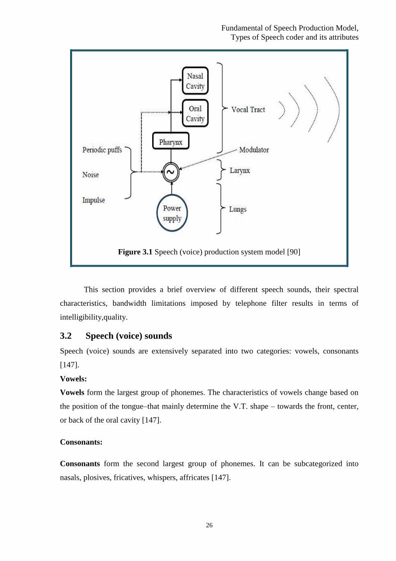
3.1 Introduction ........................................................................................................... 25
3.2 Speech (Voice) sounds..................................................................................................26
3.3 Representation of Speech Signals ......................................................................... 28
3.4 Classification of Coder .......................................................................................... 28
3.4.1 Waveform Coding .......................................................................................... 29
3.4.2 Source Coding ................................................................................................ 30
3.4.3 Hybrid Coding ................................................................................................ 31
Page 15
xv
3.5 Speech (voice) coding ........................................................................................... 31
3.6 Issues related to digital speech coding .................................................................. 33
3.7 Speech codec attributes ......................................................................................... 34
3.7.1 Transmission bit rate ........................................................................................... 34
3.7.2 Speech Quality..................................................................................................... 34
3.7.3 Bandwidth............................................................................................................ 35
3.7.4 Communication Delay ......................................................................................... 35
3.7.5 Complexity .......................................................................................................... 35
3.8 Speech codec for next-generation wireless communications................................ 36
3.9 Speech (voice) quality, intelligibility ................................................................... 36
3.9.1 Listening-only tests ............................................................................................. 36
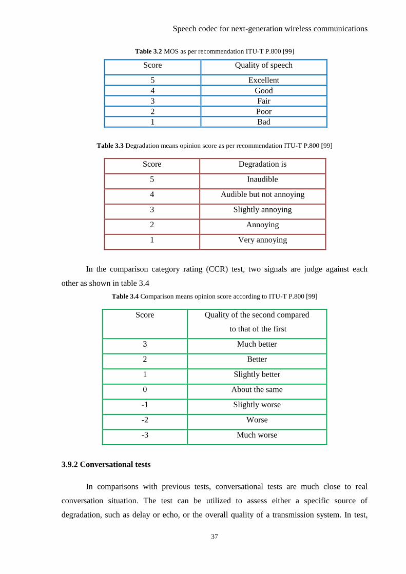
3.9.2 Conversational tests..............................................................................................37
3.9.3 Field tests ............................................................................................................. 38
3.9.4 Intelligibility tests ................................................................................................ 38
3.10 Objective quality evaluation ............................................................................... 38
3.11 Effect of B.W. on speech (voice) quality, intelligibility ..................................... 39
CHAPTER-4 ........................................................................................................................ 40
Development of Bandwidth Extension Model For W.B. To S.W.B. ................................. 40
4.1 Introduction ........................................................................................................... 40
4.2 Non-model based B.W.E. approaches................................................................... 40
4.3 B.W.E. approaches based on the source-filter model ........................................... 41
4.3.1 B.W.E. from N.B. to W.B. Speech Conversion: ................................................. 41
4.3.2 General Model for B.W.E.: ................................................................................. 41
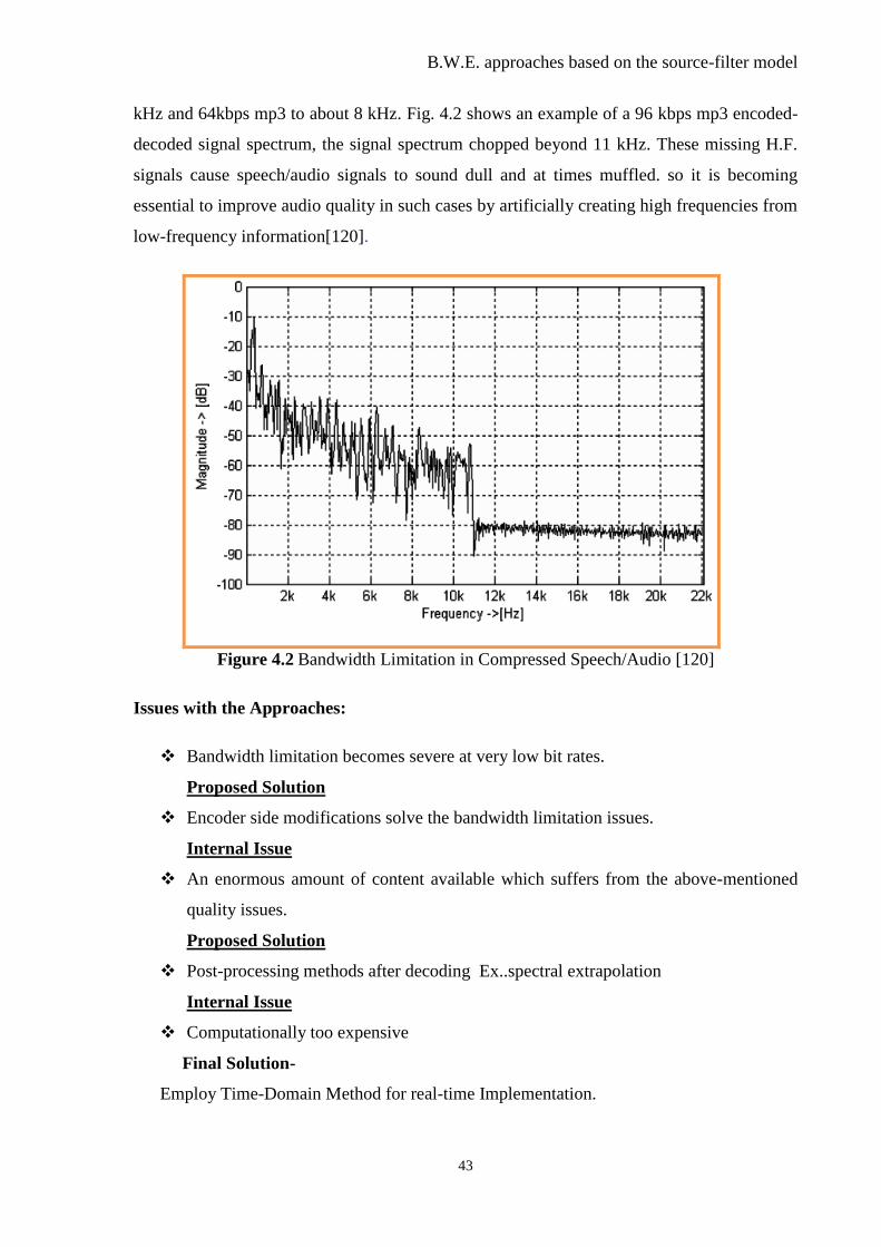
4.3.3 Bandwidth Limitation in Compressed Speech/Audio: ........................................ 42
4.3.4 Baseline System Model for B.W.E...................................................................... 44
4.4 Detailed analysis of B.W.E. based on proposed S.F.M. ....................................... 47
CHAPTER 5 ........................................................................................................................ 59
Linear prediction analysis and synthesis ............................................................................. 59
5.1 Introduction ........................................................................................................... 59
5.2 Speech file Compression based on LPC ............................................................... 59
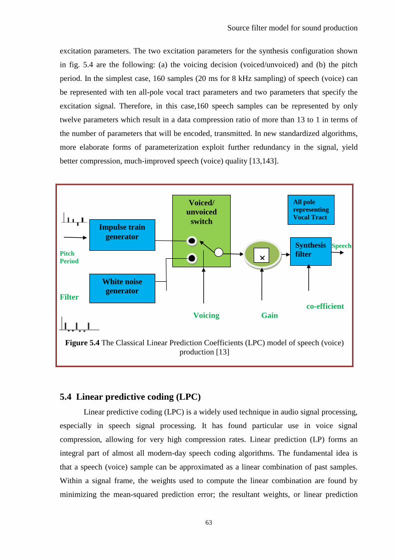
5.3 Source filter model for sound production ............................................................. 61
5.4 Linear predictive coding (LPC) ............................................................................ 63
5.5 Linear Prediction and Autoregressive Modeling .................................................. 71
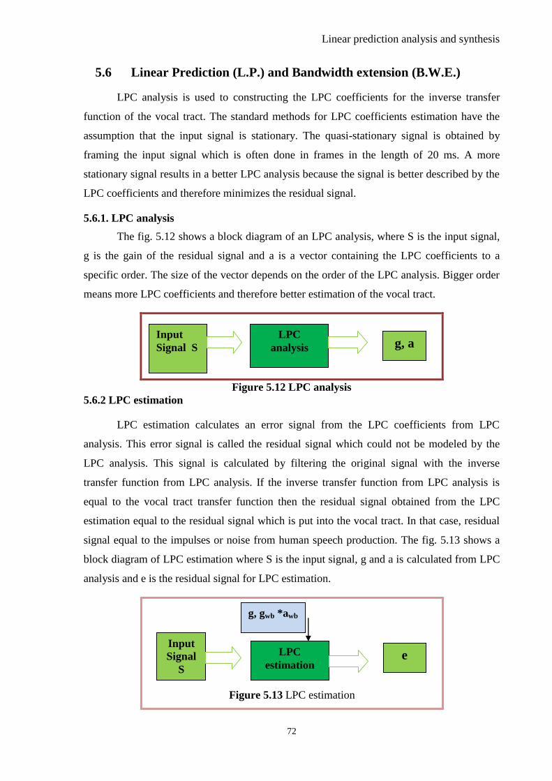
5.6 Linear Prediction (L.P.) and Bandwidth extension (B.W.E.) ............................... 72
Page 16
xvi
5.6.1. LPC analysis ....................................................................................................... 72
5.6.2 LPC estimation .................................................................................................... 72
5.6.3 LPC-synthesis ...................................................................................................... 73
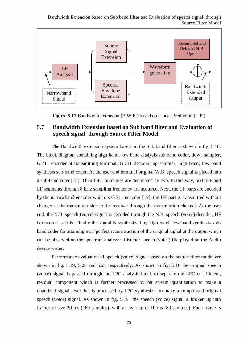
5.7 Bandwidth Extension based on Sub band filter and Evaluation of speech signal
through Source Filter Model ............................................................................................ 75
5.8 Stability consideration (LP) .................................................................................. 80
CHAPTER 6 ........................................................................................................................ 85
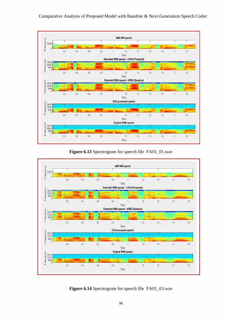
Comparative Analysis of Proposed Model with Baseline & Next-Generation Speech Codec
............................................................................................................................................. 85
6.1 Subjective & Objective Measurement for W.B. to S.W.B.................................. 85
6.2 Spectrogram .......................................................................................................... 93
CHAPTER-7 ...................................................................................................................... 100
Conclusion, Major Contribution, and Future Scope .......................................................... 100
Conclusion ..................................................................................................................... 100
Major Contribution ........................................................................................................ 101
Future Scope .................................................................................................................. 101
References .......................................................................................................................... 102
List of Publications ............................................................................................................ 113
Page 17
xvii
List of Abbreviation
Sr.
No.
Abbreviations Full Form
1
1G
1st generation
2 2G
2nd
generation
3
3G 3rd
generation
4
4G 4th
generation
5
GSM global System for mobile communications
6
3GPP 3rd generation partnership project
7
NB narrowband
8
WB wideband
9 SWB super wideband
10
AMR adaptive multi rate
11
AMR WB adaptive multi-rate wideband
12
BWE bandwidth extension
13 LTE long-term evolution
14
CCITT international telegraph and telephone
consultative committee
15 AMPS advanced mobile telephone system
16 ASR automatic speech recognition
17 PCM pulse code modulation
18 ADPCM adaptive delta pulse code modulation
19 CDMA
code division multiple access
20 CELP code-excited linear prediction
21 PSTN public switched telephone network
22 CCR comparison category rating
Page 18
xviii
23 WCDMA wideband code division multiple access
24 CS-ACELP conjugate-structure algebraic code-excited
linear prediction
25 EVS enhanced voice services
26 FFT fast Fourier transform
27 VT vocal tract
28 SFM source filter model
29 AMPS advanced mobile telephone system
30 LPC linear predictive coding
31 ITU international telecommunication union
32 ITU-T
telecommunication standardization sector of
the international telecommunication union
33 M.F.C.C. mel frequency cepstral coefficients
34 ISDN integrated services digital network
35 IMT-2000 international mobile telecommunications-
2000
36 GMM gaussian mixture model
37 HB
highband
38 HD high definition
39 HF high frequency
40 LF low frequency
41 DCR degradation category rating
42 EFR enhanced full rate
43 BPF band pass filter
44 KBPS kilo bit per second
45 MBPS megabit per second
46 MOS mean opinion score
47 MDCT modified discrete cosine transform
Page 19
xix
48 BW bandwidth
49 OLA overlap and add
50 VoIP voice over Internet Protocol
51 LTE long term evaluation
52 UMTS universal mobile telecommunication System
53 VQ vector quantization
54 PESQ perceptual evaluation of speech quality
55 CMOS complementary mean opinion score
56 RPE-LTP regular pulse excitation with long-term
prediction
57 ETSI european telecommunications standards
institute
58 WiMAX 2 worldwide interoperability for microwave
access 2
59 LTE-A long-term evolution advanced
60 VoLTE voice over long term evolution
61 FDMA frequency division multiple access
62 FB full band
63 DRT diagnostic rhyme test
64 MRT modified rhyme test
65 SRT speech reception threshold
66 ENC encoder
67 DEC decoder
68 ABS analysis-by-synthesis
69 HFBE high frequency bandwidth extension
70 SF Spectral folding
71 ST spectral translation
72 NLD non linear distortion
Page 20
xx
73 LSF line spectral frequencies
74 STFT short-time Fourier transform
75 PSD power spectral density
76 AR autoregressive
77 MOS-LQO mean opinion score linear quality objective
78 TD-CDMA time division code division multiple access
79 SNR signal-to-noise- ratio
80 EB extension band
Page 21
xxi
List of Symbols
Sr.
No.
Symbol
Description
1 Sn narrowband input signal
2 x feature extracted from narrowband input signal
3 unᶺ estimated narrowband signal from analysis filter
4 uwᶺ estimated wideband signal from synthesis filter
5 ARᶺw Estimate wideband envelope
6 e[n] error signal
7 s[n] AR signal
8 sᶺ[n] predicted AR signal
9 Xwb input wideband signal
10 Xswb estimated super wideband output
Page 22
xxii
List of Figures
Figure 1.1 A Snapshot of the mobile devices launched in various generations (1G to 4G )....
........................................................................................................................................ 2
Figure 1.2 Average speech spectrum from a 10s long speech sample of a male speaker.. ... 8
Figure 1.3 Bandwidth Extension at the Receiver Terminal................................................... 8
Figure 1.4 Spectra comparison of oiginal, N.B. & W.B. speech signal ................................ 9
Figure 1.5 Step From N.B.-W.B.-S.W.B. telephony ............................................................ 9
Figure 1.6 Missing frequency components of W.B. and N.B. signal. ................................. 11
Figure 3.1 Speech production system model. ...................................................................... 26
Figure 3.2 Representation of speech signals ........................................................................ 29
Figure 3.3 Hierarchy of speech coders ................................................................................ 30
Figure 3.4 General Block Diagram of speech coding .......................................................... 32
Figure 3.5 Voice And Unvoiced speech frame representation ............................................ 33
Figure 4.1 General Model for B.W.E. ................................................................................. 42
Figure 4.2 Bandwidth Limitation in compressed speech/audio ........................................... 43
Figure 4.3 High-Frequency Bandwidth Extension (H.F.B.E.) Algorithm ........................... 44
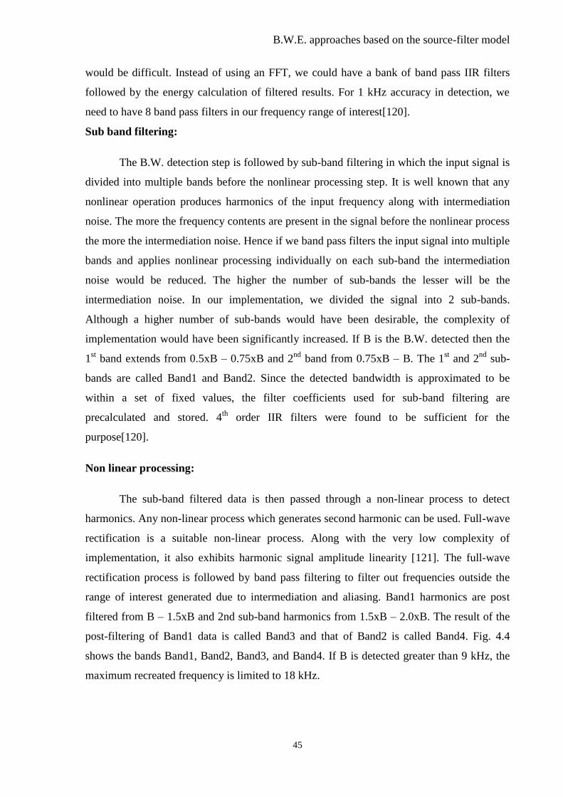
Figure 4.4 Input and Reconstruction Band .......................................................................... 46
Figure 4.5 Block Diagram of the Proposed approach for W.B. To S.W.B. ......................... 48
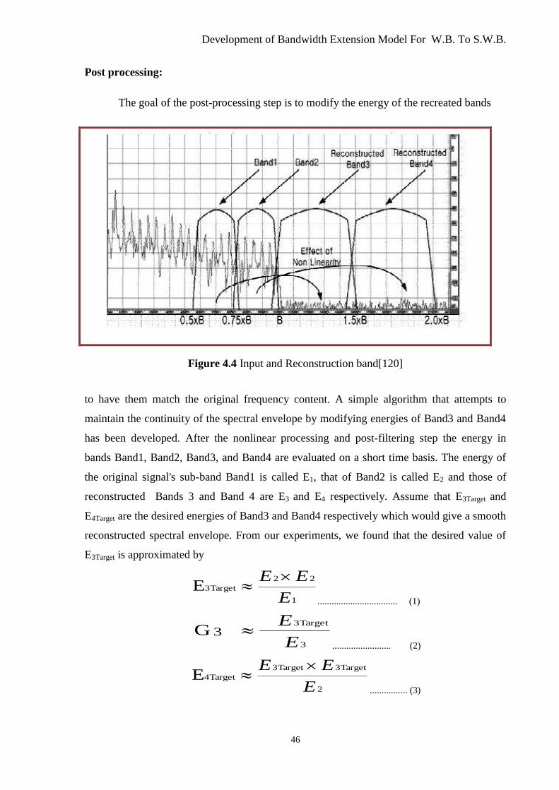
Figure 4.6 Pictorial representation for Framing. .................................................................. 49
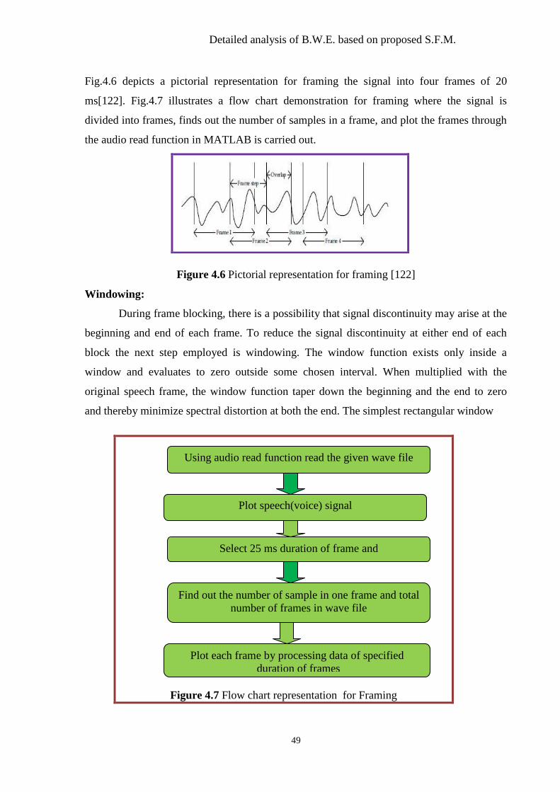
Figure 4.7 Flow chart representation for Framing .............................................................. 49
Figure 4.8 All Pole spectral shaping synthesis filter ............................................................ 50
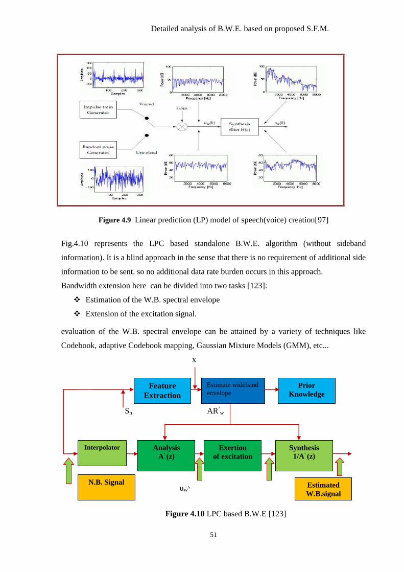
Figure 4.9 Linear Prediction (LP) Model of speech creation. ............................................. 51
Figure 4.10 LPC based B.W.E. ............................................................................................ 51
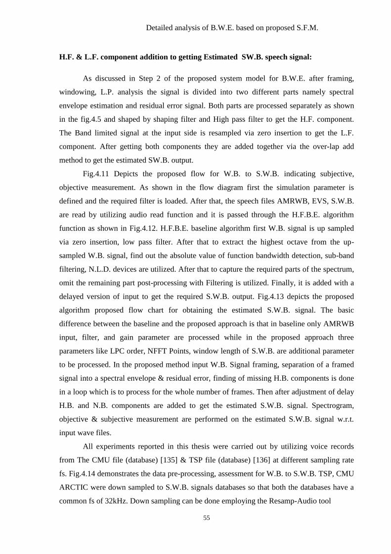
Figure 4.11 Proposed Flow for W.B. to S.W.B. .................................................................. 56
Figure 4.12 Baseline Algorithm Proposed Flow Chart ........................................................ 56
Figure 4.13 Proposed Algorithm Proposed Flow Chart....................................................... 57
Figure 4.14 Data Pre-Processing and Assessment for W.B. to S.W.B................................58
Figure 5.1 LPC co-efficient obtained from Input speech signal .......................................... 59
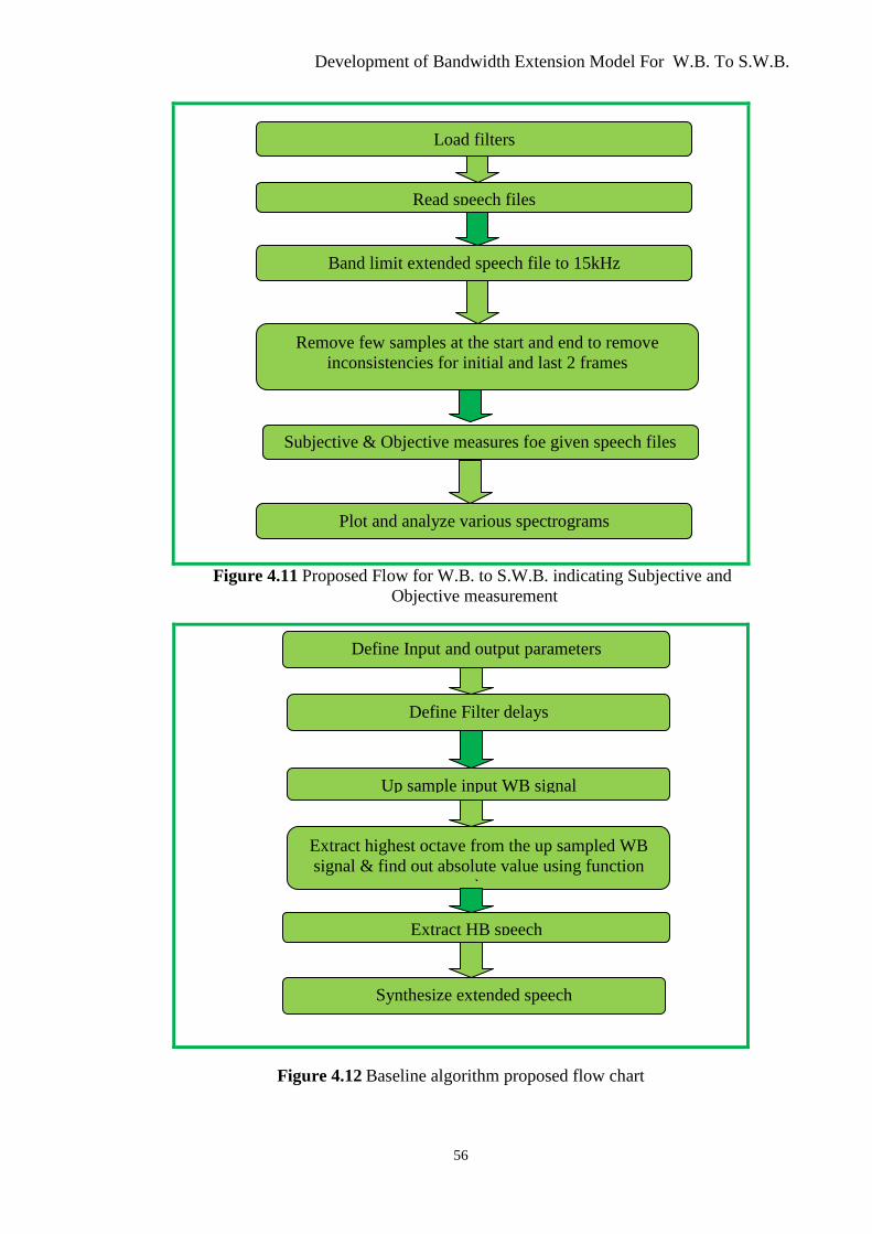
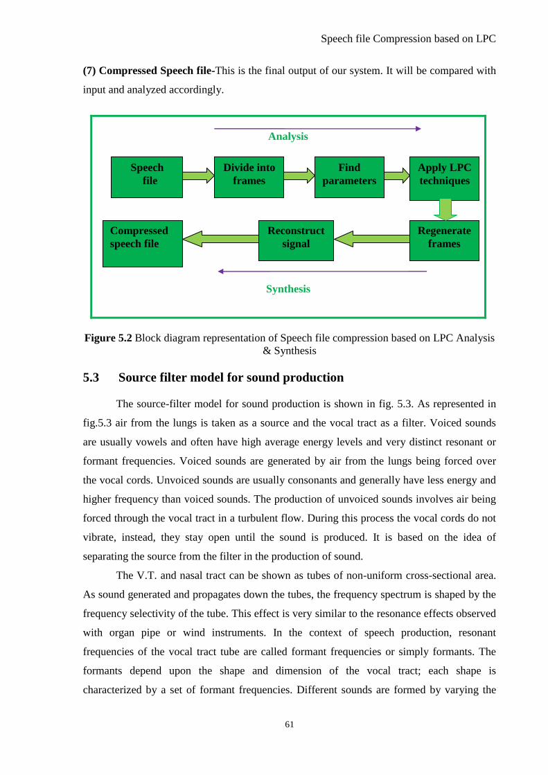
Figure 5.2 Block Diagram representation of speech file compression based on LPC Analysis
& Synthesis ................................................................................................................... 61
Figure 5.3 Source Filter Model for Sound Production ........................................................ 62
Figure 5.4 Classical Linear Prediction Coefficients (LPC) Model of Speech Production .. 63
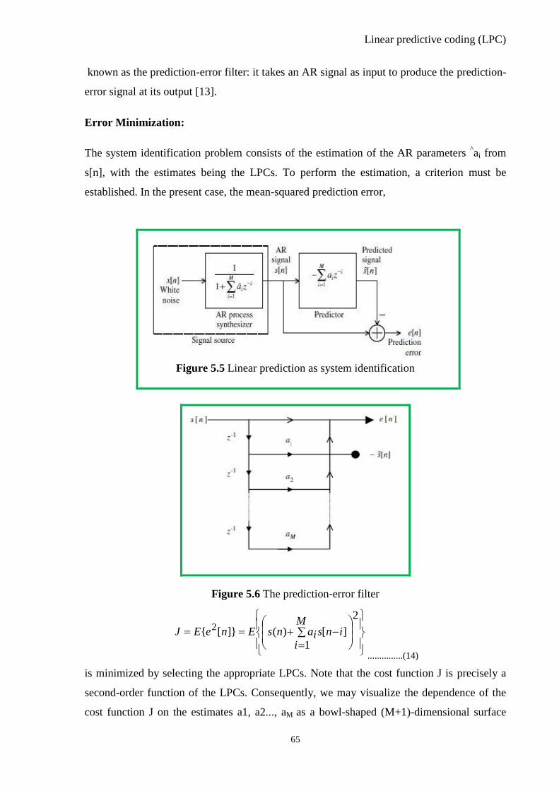
Figure 5.5 Linear Prediction as System Identification ......................................................... 65
Page 23
xxiii
Figure 5.6 Prediction-Error Filter ........................................................................................ 65
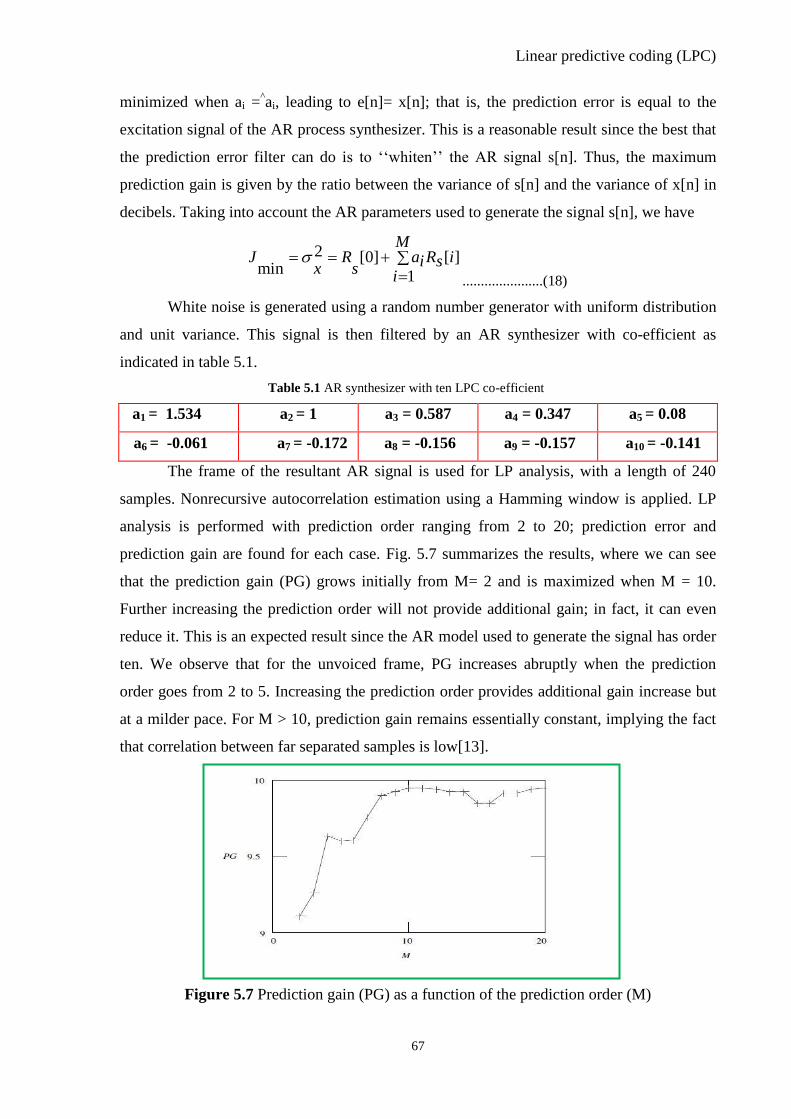
Figure 5.7 Prediction Gain (PG) as a function of the Prediction Order (M) ....................... 67
Figure 5.8 A Plot of PG Vs Prediction Order (M) for the signal Frames ............................ 68
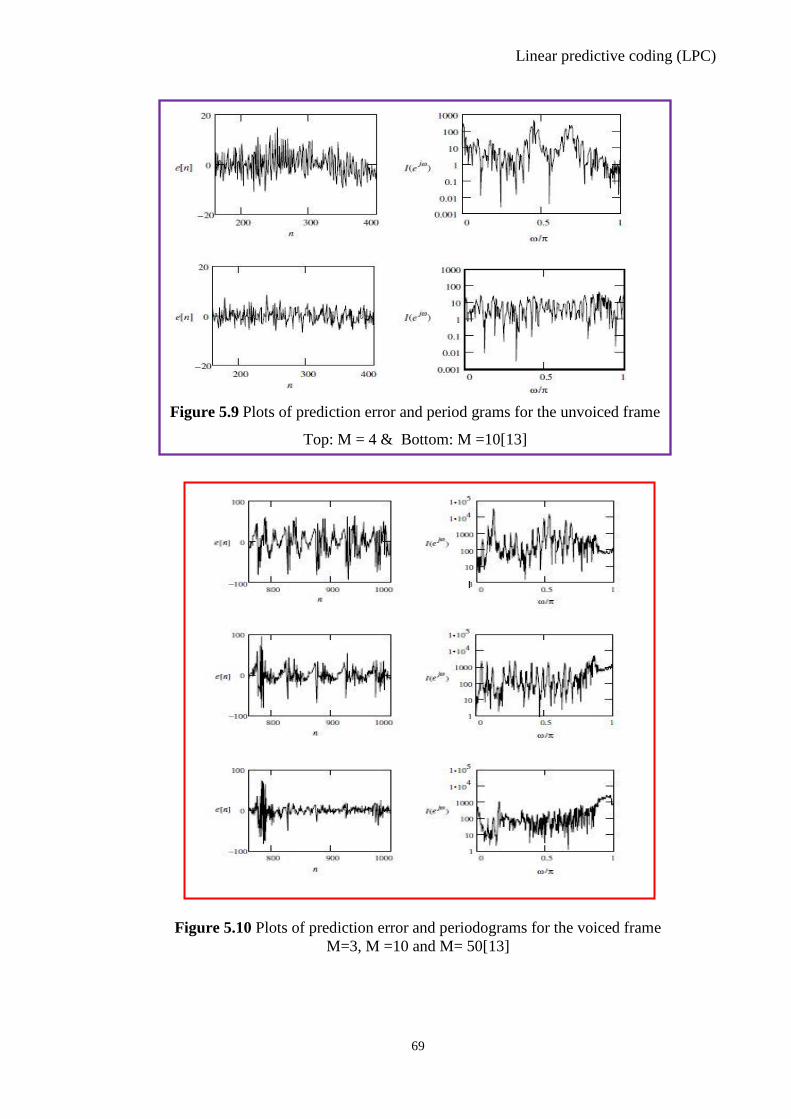
Figure 5.9 Plots of Prediction Error and Periodograms for the Voiced Frame .................... 69
Figure 5.10 Plots of Prediction Error and Periodograms for the Unvoiced Frame.............. 69
Figure 5.11 Plot of PSD for M=2, M=10,M=20 .................................................................. 70
Figure 5.12 LPC Analysis .................................................................................................... 72
Figure 5.13 LPC Estimation ................................................................................................ 72
Figure 5.14 LPC Synthesis .................................................................................................. 73
Figure 5.15 Input Signal before LPC Analyzer and Input Signal After LPC Synthesizer with
Error Signal................................................................................................................... 73
Figure 5.16 Complete Block Diagram of B.W.E. Output from Band-Limited N.B. Signal 74
Figure 5.17 Bandwidth Extension (B.W.E.) Based on Linear Prediction (LP) ................... 75
Figure 5.18 Bandwidth Extension Based on Sub Band Filter ............................................. 76
Figure 5.19 Performance Evaluation of speech signal Based on Source Filter Model ........ 77
Figure 5.20 Source Filter Model-based Analysis ................................................................ 77
Figure 5.21 Source Filter Model-based Synthesis ............................................................... 77
Figure 5.22 I/P Time-Domain Waveform of Wave File ''Om Shri Ganeshay Namah'' ...... 78
Figure 5.23 O/P Time-Domain Waveform of Wave File "Om Shri Ganeshay Namah" ..... 78
Figure 5.24 Input Frequency Domain Waveform of Wave file "Om Shri Ganeshay Namah"
...................................................................................................................................... 78
Figure 5.25 O/P Freq. Domain Waveform of Wave file "Om Shri Ganeshay Namah" ...... 79
Figure 5.26 Pre-Emphasized speech signal ......................................................................... 79
Figure 5.27 A Hamming Windowed speech signal ............................................................. 79
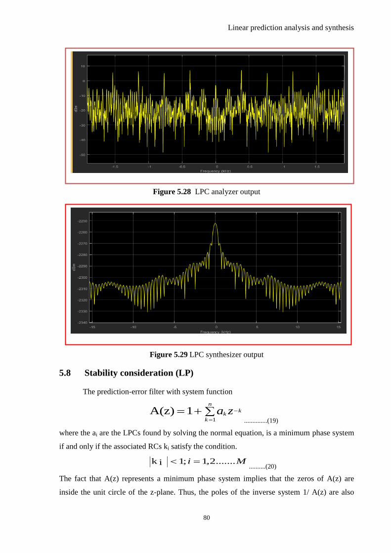
Figure 5.28 LPC Analyzer Output ....................................................................................... 80
Figure 5.29 LPC Synthesizer Output ................................................................................... 80
Figure 5.30 Auto Cor-Relation co-efficient, Reflection co-efficient & LPC co-efficient ... 81
Figure 5.31 Short-Term Prediction-Error filter connected in series to a Long-Term
Prediction-Error Filter .................................................................................................. 82
Figure 5.32 Block Diagram of the Synthesis filter .............................................................. 82
Figure 6.1 MOS-L.Q.O. For Proposed, H.F.B.E., L.P._Order=12,16,24 & E.V.S. Algorithm
for Bdl_Arctic_A0001.wav .......................................................................................... 88
Figure 6.2 P.E.S.Q. For Proposed, H.F.B.E., L.P._Order=12,16,24 & E.V.S. Algorithm For
Bdl_Arctic_A0001.wav ................................................................................................ 89
Page 24
xxiv
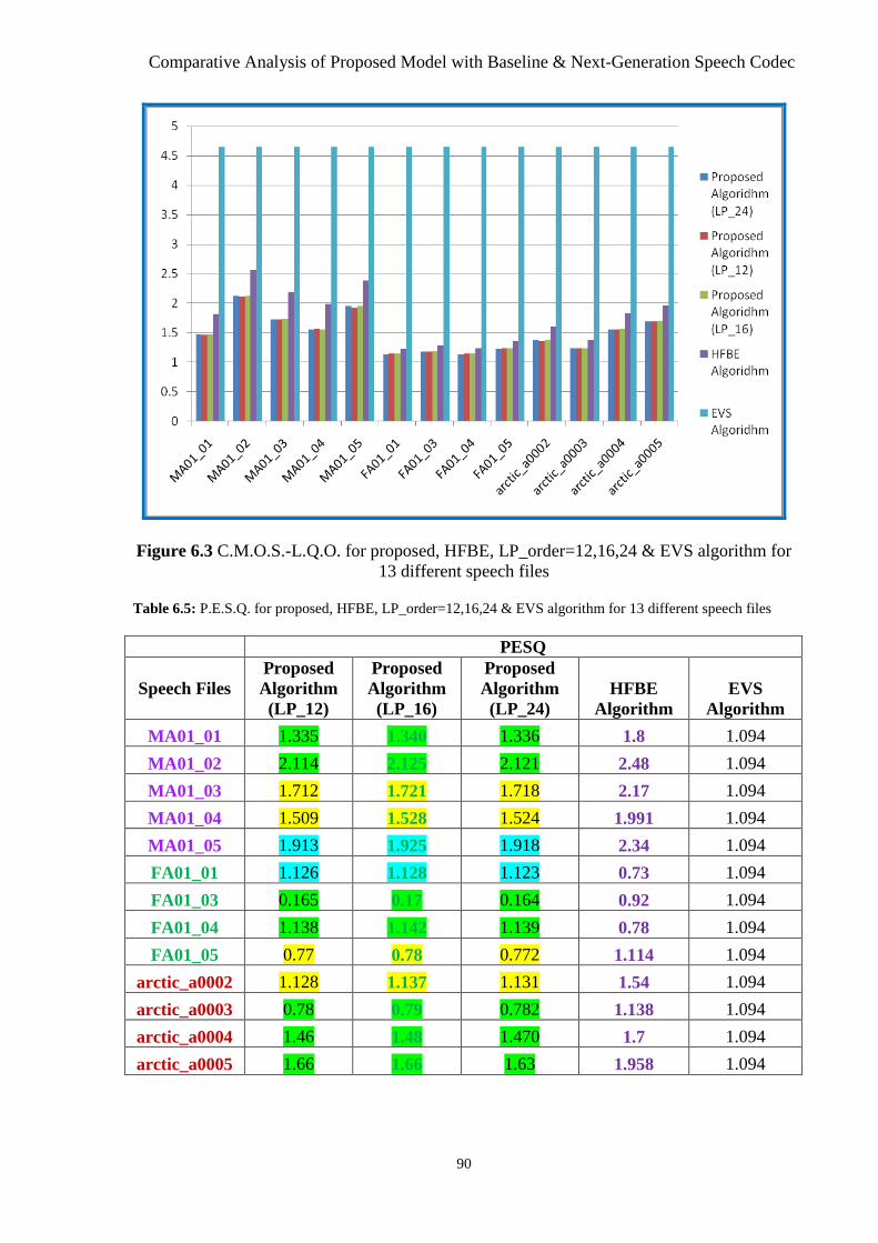
Figure 6.3 MOS-L.Q.O. For Proposed, HFBE, LP_Order=12,16,24 & EVS Algorithm For
Thirteen Different Speech Files .................................................................................... 90
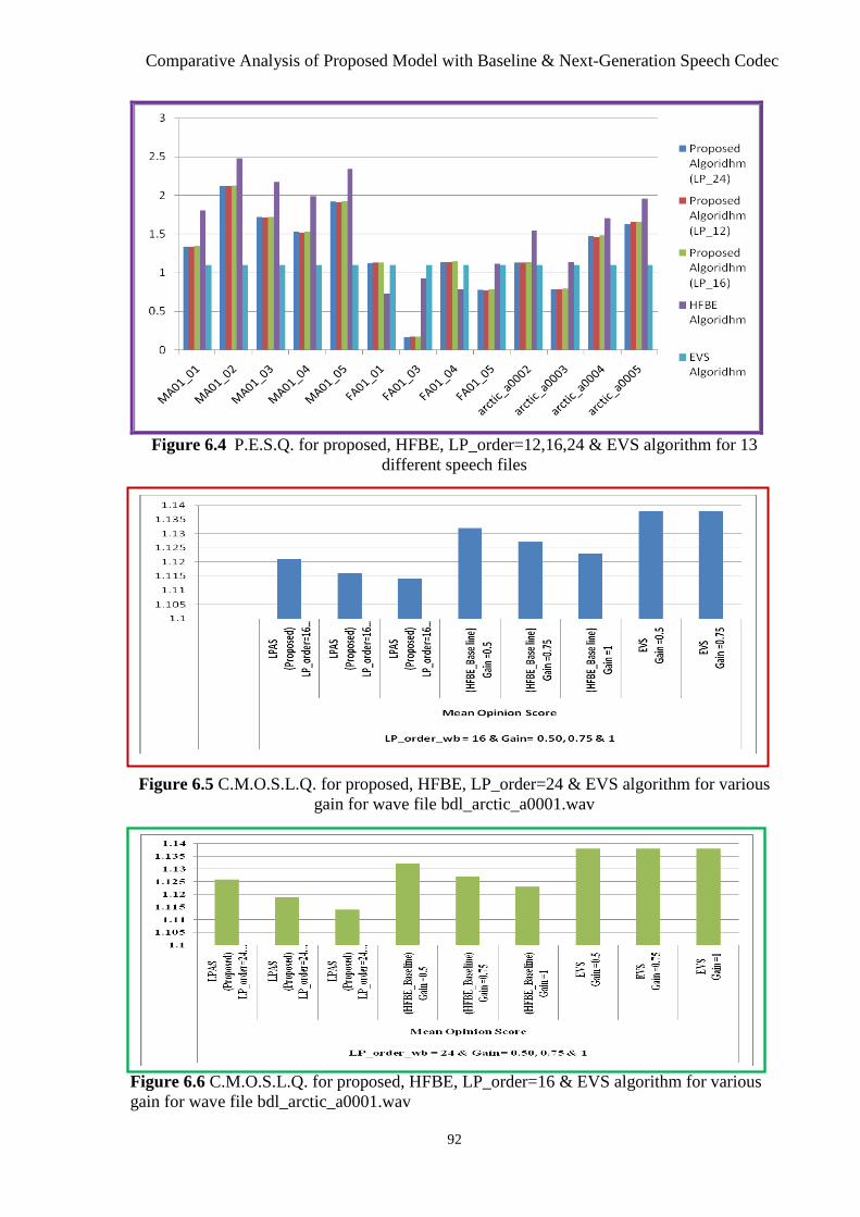
Figure 6.4 P.E.S.Q. For Proposed, HFBE, LP_Order=12,16,24 & EVS Algorithm For
Thirteen Different Speech Files .................................................................................... 92
Figure 6.5 M.O.S.L.Q. For Proposed, HFBE, LP_Order=24 & EVS Algorithm For Various
Gain For Wave File Bdl_Arctic_A0001.wav ............................................................... 92
Figure 6.6 M.O.S.L.Q. For Proposed, HFBE, LP_Order=16 & EVS Algorithm for Various
Gain For Wave File Bdl_Arctic_A0001.wav ............................................................... 92
Figure 6.7 M.O.S.L.Q. For Proposed, HFBE, LP_Order=12 & EVS Algorithm for Various
Gain For Wave File Bdl_Arctic_A0001.wav ............................................................... 93
Figure 6.8 Spectrogram for Speech File Ma01_01.wav .................................................... 93
Figure 6.9 Spectrogram for Speech File Ma01_02.wav ..................................................... 94
Figure 6.10 Spectrogram for Speech File Ma01_03.wav ................................................... 94
Figure 6.11 Spectrogram for Speech File Ma01_04.wav ................................................... 95
Figure 6.12 Spectrogram for Speech File Ma01_05.wav ................................................... 95
Figure 6.13 Spectrogram for Speech File Fa01_01.wav..................................................... 96
Figure 6.14 Spectrogram for Speech File Fa01_03.wav..................................................... 96
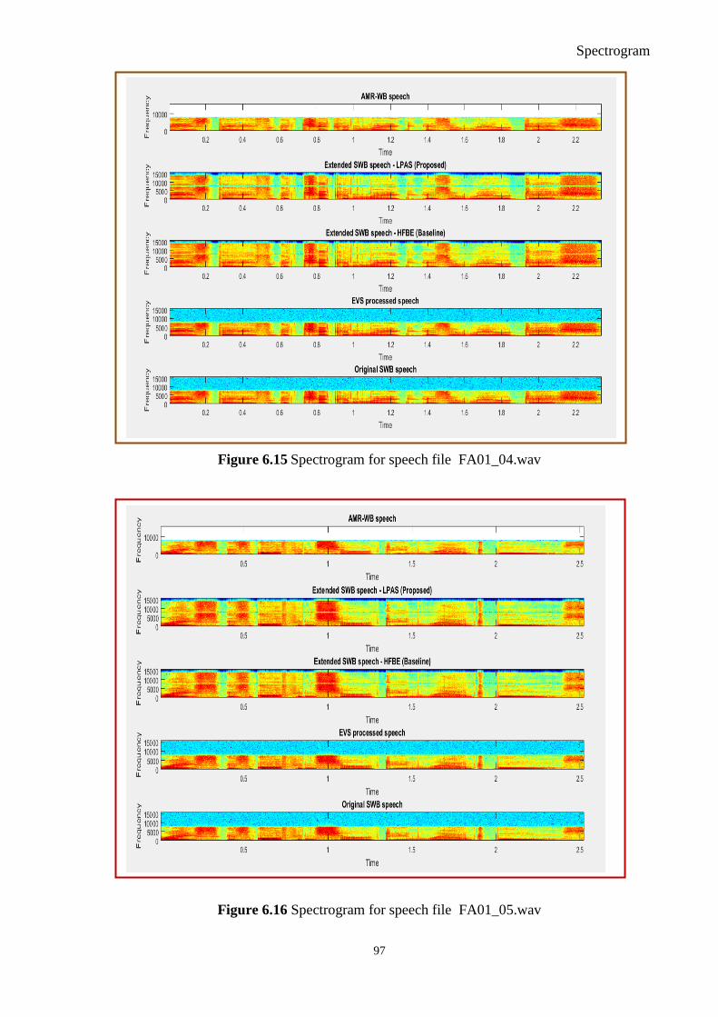
Figure 6.15 Spectrogram for Speech File Fa01_04.wav..................................................... 97
Figure 6.16 Spectrogram for Speech File Fa01_05.wav..................................................... 97
Figure 6.17 Spectrogram for Speech File Arctic-A0002.wav ............................................ 98
Figure 6.18 Spectrogram for Speech File Arctic-A0003.wav ............................................ 98
Figure 6.19 Spectrogram for Speech File Arctic-A0004.wav ............................................ 99
Figure 6.20 Spectrogram for Speech File Arctic-A0005.wav ............................................. 99
Page 25
xxv
List of Tables
Table 3.1 MOS Quality Rating ..................................................................................... 35
Table 3.2 Mean Opinion Score according to ITU-T P.800 ......................................... 37
Table 3.3 Degradation Means Opinion Score according to ITU-T P.800 ................... 37
Table 3.4 Comparison Means Opinion Score according To ITU-T P.800 .................. 37
Table 5.1 AR Synthesizer With ten LPC co-efficient .................................................. 67
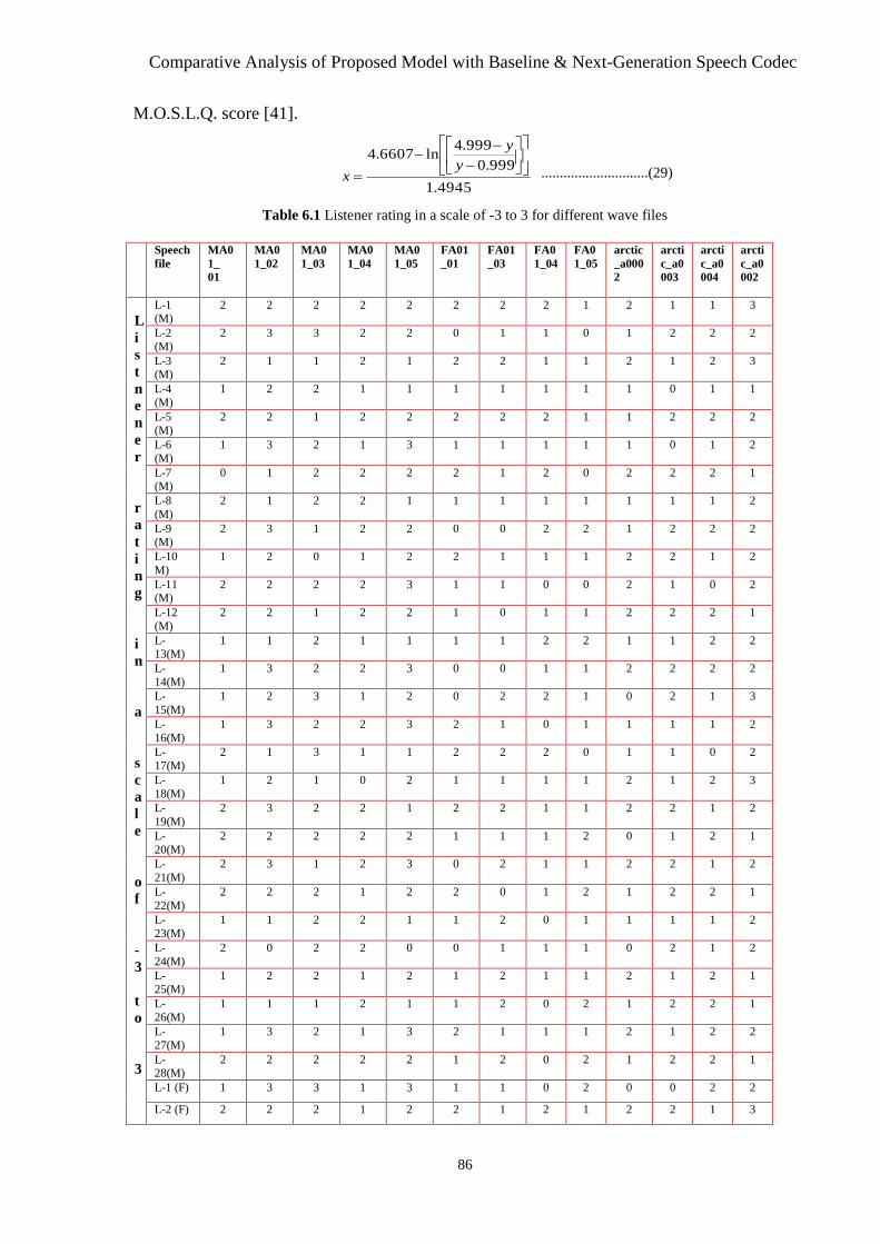
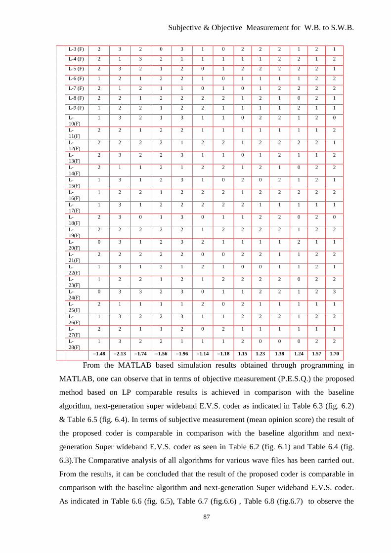
Table 6.1 Lister Rating in a Scale of -3 to 3 for different wavefiles.............................78
Table 6.2 MOS-L.Q.O. for Proposed, H.F.B.E., LP_Order=12,16,24 & E.V.S. algorithm
for bdl_arctic_a0001.wav ............................................................................................ 88
Table 6.3 P.E.S.Q. For Proposed, H.F.B.E., LP_Order=12,16,24 & E.V.S. algorithm for
bdl_arctic_a0001.wav ................................................................................................... 89
Table 6.4 MOS-L.Q.O. for Proposed, H.F.B.E., LP_Order=12,16,24 & E.V.S. algorithm
for Thirteen different speech files ................................................................................ 89
Table 6.5 P.E.S.Q. for Proposed, H.F.B.E., LP_Order=12,16,24 & E.V.S. algorithm for
Thirteen different speech files ...................................................................................... 90
Table 6.6 M.O.S.L.Q. for Proposed, H.F.B.E., LP_Order=24 & E.V.S. algorithm for
various Gain for wave file bdl_arctic_a0001.wav ........................................................ 91
Table 6.7 M.O.S.L.Q. For Proposed, H.F.B.E., LP_Order=16 & E.V.S. algorithm For
various Gain for wave file bdl_arctic_a0001.wav ........................................................ 91
Table 6.8 M.O.S.L.Q. For Proposed, H.F.B.E., LP_Order=12 & E.V.S. algorithm For
various Gain for wave file bdl_arctic_a0001.wav ........................................................ 91
Page 27
Fruition of Communication Systems
1
CHAPTER-1
Introduction
1.1 Fruition of Communication Systems
As the imperative of the remote transmission recurrence band assets due to the
complexity of the 3G versatile communications environment, reproduced speech (voice)
quality, comprehensible at the recipient side is found hardened, scarcely capable of being
heard, thin since of the constrained transmission capacity of 300-3.4KHz. In contrast,
Today's terminals, infrastructure, operate at wider bandwidths for which speech (voice)
quality, intelligibility are greatly improved. Normally, the total move from narrowband (300-
3.4KHz) to wideband (0.05-7kHz) and wideband (0.05-7kHz) to super-wideband (0.05-
14kHz) communications will require impressive time. As a result, wideband, super-
wideband innovation must interoperate with narrowband innovation. In this case, clients will
involvement significant varieties in speech (voice) quality and intelligibility. This chapter
discusses brief highlight of fruition of communication system followed by contribution,
organization of thesis.
1.1.1 Analog , Digital telephony
The limited N.B. speech (voice) signals, were sent out over different frequency
channels with a frequency separation of 4kHz. The first wireless speech (voice) transmission
started in year 1915 [1]. In year 1937, Alex Reeve has visualized time-division multiplexing
based pulse code modulation (PCM) which has shaded light for voice communication
digitization [2]. The commercial utilization of PCM was started in the year 1950s [3]. By the
existing PSTNs, PCM adopted the typical N.B. B.W. for communication. So, for long period
of times, subscribers were offered only N.B. communication services.
1.1.2 Wireless Cellular Networks
After Marconi's doing well attempt at wireless transmission, engineers, academicians,
scientists started to carry out the research and development ( R & D) activity for R.F. based
proficient communication [1]. The 1st
generation (1G) wireless mobile phone system was
developed in 1973, but not commercialized until year 1984. Wireless communications have
Page 28
Introduction
2
remarkably gone ahead in last few years. Mobile handsets have also advanced together with
the generations (from 1G to 4G) with added functionalities.
Fig. 1.1 depicts a snapshot of the mobile devices launched in various generations (1G
to 4G). The first generation cellular systems, introduced in the year 1980s, used analog
cellular, cordless telephone technology [2]. Second-generation (2G) systems, arrived in year
1980s, used digital speech (voice) transmission. 2G services played a vital role for voice
transmission which was inefficient for data transmission [4].Third-generation (3G) systems
entered in market in the year 2000. It provides advanced voice, high-speed data services in
comparisons with Second-generation (2G) systems. It utilized packet switching for data
transmission while circuit-switching for voice transmission. Universal Mobile Tele-
communication System (UMTS) or wideband CDMA (WCDMA), time division-
synchronous CDMA (TD-SCDMA), CDMA2000 are the most popular 3G technologies [4].
Packet switching technology employed in fourth generation (4G) systems supports 100Mbps
data rate. It is used in system for voice as well as data services. WiMAX 2, LTE-Advanced
are the two most popular 4G protocols [4]. Third as well as fourth generation wireless
communication (W.C.) system are becoming popular in the world market due to their low bit
rate coder. It was proposed to provide interactive multimedia communication including
teleconferencing, internet access an combination of another benefit that gets to be practicable
with low complex, low cost, low bit rate, less processing delay. So one can articulate that
these are the major attributes that play a vital role while designing any particular coder.
Figure 1.1 A snapshot of the mobile devices launched in various generations [5]
Page 29
Fruition of Communication Systems
3
1.1.3 Speech Coding
Speech coding is defined as the procedure of shrinking the bit rate of digital speech
(voice) signal representation for communication or storage while maintaining a speech
(voice) quality adequate for the application [6]. In general, it is the way to represent the
speech (voice) signal with the fewest number of bits, while maintaining a sufficient level of
quality of the retrieved or synthesized speech with reasonable computational complexity. To
achieve high-quality speech at a low bit rate, one can apply coding algorithm (a sophisticated
method to reduce the redundancies from the speech signal).
Although wide-bandwidth channels, networks are becoming more viable, speech
(voice) coding for bit-rate reduction has retained its importance due to the need for low bit
rates for cellular, Internet communications over constrained-bandwidth channels, voice
storage systems. Due to the increasing demand for digital speech communication, speech
coding technology has received augmenting levels of interest from the research and
standardization. Speech coding standards have played, and continued to play an important
role in the development, use of speech codes. There are a few speech coding applications in
which inter-operatability is not an issue. An example of such an application is a digital
answering machine or digital voice mail system in which the same system is used to both
encode, decode the speech. For such applications, the speech coder of choice can be the best,
most cost-effective available at the time when the system is designed, without regard to
inter-operatability. For the vast majority of applications, however, inter-operatability is a
major issue. All telecommunications applications belong to this class. For inter-operatability
to be achieved, standards must be defined as well as implemented. This encourages the
research community to investigate alternative techniques for speech (voice) coding with the
objectives of overcoming deficiencies. The standardization community pursues the
establishment of standard speech coding methods for various applications that will be
widely accepted, implemented by the industry. A variety of standards bodies have been
responsible for the definition of new standards. Speech (voice) coding can be categorized
based on equipped bandwidth.
N.B. coding:
N.B. coding techniques squeeze speech (voice) signals in the range of 0.3-3.4kHz [7].
Page 30
Introduction
4
Pulse-code modulation (PCM):
PCM is a waveform coding technique that carries out discrete-time, magnitude
approximation of continuous signals in the time field [8]. ITU- recommendation G.711 [9],
G.712 [10] normalized the transmission characteristics of PCM for speech (voice) signals.
Parametric coders (L.P.C.) code a set of model parameters in place of the time domain
waveforms. To take benefit of both the schemes, the combination of both the coding method,
hybrid method can be utilized. In this method co-efficient of synthesis filter are sent as a side
information while quantization of L.P. residual error (difference between actual and
predicted sample difference) is done via CELP coding [11].
For economical, complexity reasons, bit rate reduction from 64kbps is a most
important requirement [11]. ITU-T- recommendation G.726 [12] homogenized an PCM
extension known as ADPCM [12]. ADPCM supports multiple bit rates of 16, 24, 32 &
40kbps. In ADPCM quantization of error signal is carried out [13].
GSM full-rate (GSM-FR), enhanced full-rate (EFR) codec:
GSM full rate (GSM-FR) codec relies on LPC has employed short-term LP analysis
for spectral envelope modeling, long-term LP analysis to attain a residual error signal. The
Quantization of attained signal is done through ADPCM which operates at 13kbps was
adopted by ETSI-recommendation GSM 06.10 [14]. In year 1992, GSM-FR was further
improved using a well-organized V.Q. system for residual error signal using ACELP
algorithm [15-16]. It was normalized as GSM-EFR codec in ETSI- recommendation GSM
06.60 [17] in 1996, operates at 12.2kbps. The GSM-EFR codec achieved speech (voice)
quality comparable with ADPCM at 32kbps [11].
G.729:
It is normalized in ITU-T-recommendation G.729 [18] that in the year 1995, it was
operated at 8kbps. The codec was based on conjugate-structure ACELP which was widely
employed in VOIP infrastructures.
Adaptive multi-rate (AMR):
An expansion of the EFR codec with eight possible bit rates ranging from 4.75 to
12.2 kbps, was standardized by ETSI Recommendation GSM 06.90 for 2G & 3G system
[19]. 3GPP takes up AMR as the default speech (voice) codec for 3G wideband systems
Page 31
Fruition of Communication Systems
5
(UMTS, CDMA2000) as mentioned in 3GPP TS 26.090 [20]. AMR coding occupies the
transcoding of AMR-coded speech (voice) signals to/from PCM format [21].
Wideband coding:
As W.B. transmission improves the quality of voice transmission, there is a rising
demand for W.B. communication services in fixed, mobile networks at lower bit rates. The
first W.B. speech codec (voice) for ISDN, tele-conferencing was homogenized in year 1985
by CCITT [11]. The ITU-T recommendation G.722 [22] spell out the characteristics of an
audio W.B. coding system in which a frequency band is split into two, lower and higher,
sub-bands in a way that both are encoded using sub band ADPCM. The G.722 standard is
employed as a benchmark for other codec assessment [13]. In the year 1999, a low-
complexity W.B. codec was commenced in ITU-T recommendation G.722.1 [23]. Low-
complexity W.B. codec attained as good as speech (voice) quality at reduced bit rates of
24kbps, 32 kbps.
Adaptive multi-rate wideband (AMRWB):
AMRWB encodes speech (voice) within a bandwidth of 0.05-7kHz. The AMRWB
codec relies on the ACELP technique was first standardized in the year 2001 by 3GPP TS
26.190 [24] for 3G systems. It utilizes B.W.E. for signal re-synthesis beyond 6.4kHz as
specified in ITU-T recommendation G.722.2 [25]. It supports nine-bit rates ranging from 6.6
to 23.85 kbps but achieves higher speech quality at 8.85 kbps in comparisons with AMR at
12.2kbps [26]. Speech (voice) transmission by AMRWB provides significantly better quality
than N.B. due to B.W. expansion results in much more natural sound. By May 2016, 164
mobile operators (17 on GSM (2G), 130 on UMTS (3G), 63 on LTE (4G) networks) have
commenced commercial HD voice services in 88 countries [21].
G.729.1:
ITU-T Recommendation G.729.1 [27] sanctify an extension to the G.729 codec
provide scalable N.B.,W.B. coding of speech (voice), audio signals from 8-32kbps [28].
S.W.B. or F.B. coding:
S.W.B. or F.B. speech (voice) communications send out almost complete human
speech (voice) spectrum results in much more natural, understandable speech (voice) sound
Page 32
Introduction
6
in comparisons with N.B. or W.B. communications..
G.729.1 Annex E:
G.729.1 Annex E [29] broadens the 32kbps mode of the G.729 codec to S.W.B. mode
providing bit rates in the range of 36-64kbps. An S.W.B. extension to the scalable W.B.
codec G.729.1 proposed in [30] achieve improved audio quality in comparisons with
existing S.W.B. extension G.722.1 Annex E.
Extended AMRWB (AMRWB+):
The AMRWB standard (3GPP TS 26.290 [31]) is a S.W.B.E. to the AMRWB codec
operates up to an augmented frequency range of 16kHz, bit rates up to 32kbps [14]. It is a
mixture of two codec (hybrid codec) that combines linear predictive, transform coding
techniques depending on the signal type, e.g., speech (voice) or audio [32].
G.719:
A low-complexity coding algorithm for F.B. speech (voice), audio signals is
described in ITU-T recommendation G.719. The coding technique offers bit rate from 32 to
128 kbps. [33]
HE-AAC:
The high-efficiency advanced audio codec (HE-AAC) makes use of spectral band
replication (SBR) approach for efficient coding of audio signals [34-36]
Over the top (O.T.T.) conversational codec:
O.T.T. service providers (Skype) give point-to-point services intended for voice over
internet protocol. The utilization of SILK codec allows, conventional N.B. speech (voice)
services to be transferred towards W.B., S.W.B. communications via the use of broadband IP
services [37]. OPUS is another high-quality codec which carry out hybrid coding,. OPUS
involves the coding of frequency up to 8kHz using the SILK codec, while above 8kHz
frequency are coded using CELT [39]. It gives S.W.B. or F.B. transmission at, above 24
kbps[37].
Page 33
Fruition of Communication Systems
7
Enhanced voice services (EVS) codec:
3rd
generation partnership project (3GPP) has carried out a study in the year 2010
regarding EVS codec [38]. The homogenization of it was done in year 2014. EVS codec can
encode a speech (voice) as well as other audio signals with an S.W.B. (0.05-14kHz) at bit
rates as low as 9.6kbps [28]. It operates at four different B.W. (i.e. N.B. (0.02-4kHz), W.B.
(0.05-7kHz), S.W.B. (0.05-16kHz), F.B. (0.05-20kHz) [37]). EVS supports twelve bit rates
ranging from 5.9 to 128 kbps with S.W.B., F.B. services starting at or above 9.6, 16.4kbps
correspondingly [48]. Subjective listening tests show that EVS outperforms in comparisons
with all existing conversational voice, audio codec across all bit rates, B.W. [39]. Detailed
technical details of EVS can be found in [40-43]. In upcoming scenario of advancement in
next generation wireless communication system due to the key features provided by the EVS
codec, mobile operators have started enabling their networks for EVS support [44].
1.1.4 Background on Digital Speech Transmission
In digital signal processing (DSP), signals are band-limited w.r.t. use of sampling
frequency. In analog telephone speech, B.W. is limited to 300-3.4 kHz. Due to our human
hearing system's ability to detect fundamental frequency based on the harmonics present in
the signal, the researchers, academicians have always targeted towards high frequency
compared to low frequency. Also from a speech quality & intelligibility point of view, high-
frequency content is much more significant than low frequency.
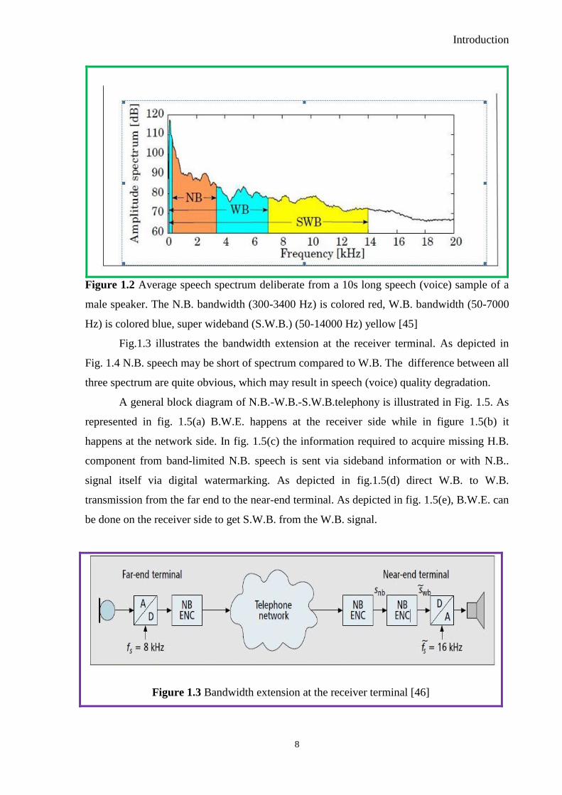
Fig.1.2 depicts the average speech (voice) spectrum deliberate from a 10s long
speech (voice) sample of a male speaker [45]. From the diagram one can say that amount of
information in N.B. is small compare to W.B. & S.W.B. In W.B amount of information is
more compare to N.B. & less compare to S.W.B. By investigating at various levels, the
researcher has found that B.W. limitation of transmitted speech (voice) resulting in much
inferior quality compares to face to face conversion due to diminution in speech (voice)
quality & intelligibility.
1.1.5 Background on Bandwidth Extension
In the recent scenario of advancement in the next-generation wireless communication
systems, due to missing high band (H.B.) component information, limitation of N.B. to
represent consonant sound speech (voice) signal looks like stiffened, barely audible & slim.
Page 34
Introduction
8
Figure 1.2 Average speech spectrum deliberate from a 10s long speech (voice) sample of a
male speaker. The N.B. bandwidth (300-3400 Hz) is colored red, W.B. bandwidth (50-7000
Hz) is colored blue, super wideband (S.W.B.) (50-14000 Hz) yellow [45]
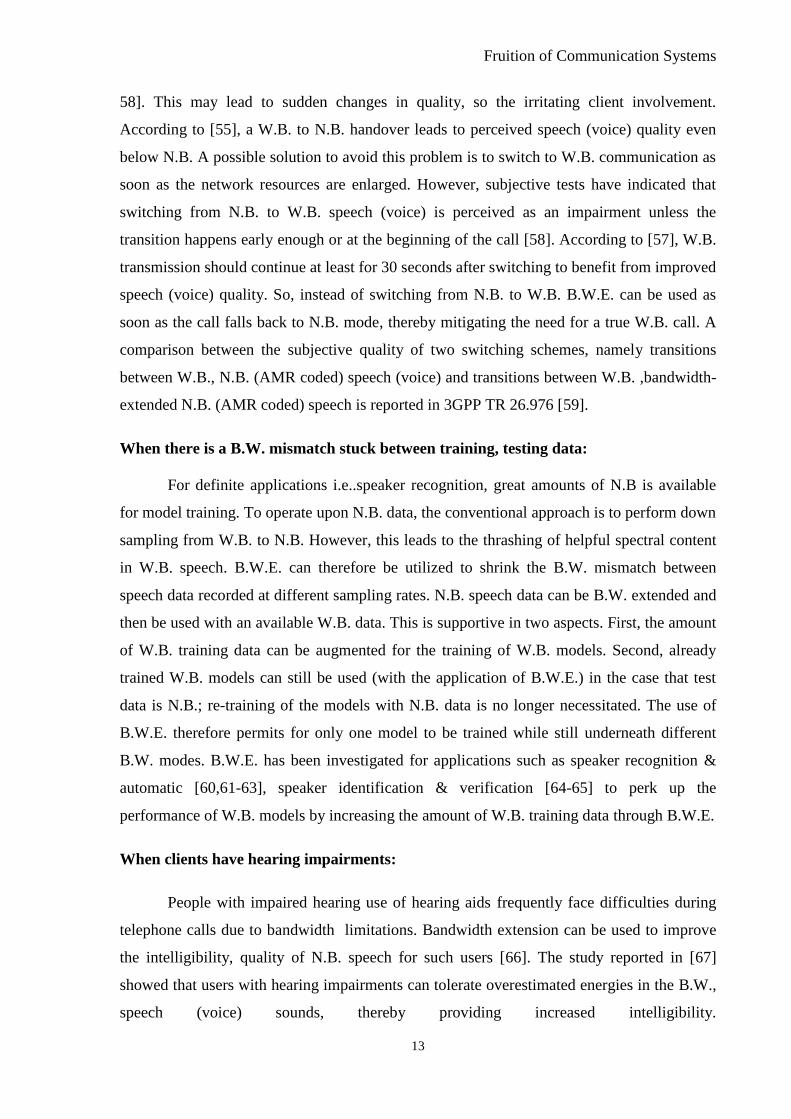
Fig.1.3 illustrates the bandwidth extension at the receiver terminal. As depicted in
Fig. 1.4 N.B. speech may be short of spectrum compared to W.B. The difference between all
three spectrum are quite obvious, which may result in speech (voice) quality degradation.
A general block diagram of N.B.-W.B.-S.W.B.telephony is illustrated in Fig. 1.5. As
represented in fig. 1.5(a) B.W.E. happens at the receiver side while in figure 1.5(b) it
happens at the network side. In fig. 1.5(c) the information required to acquire missing H.B.
component from band-limited N.B. speech is sent via sideband information or with N.B..
signal itself via digital watermarking. As depicted in fig.1.5(d) direct W.B. to W.B.
transmission from the far end to the near-end terminal. As depicted in fig. 1.5(e), B.W.E. can
be done on the receiver side to get S.W.B. from the W.B. signal.
Figure 1.3 Bandwidth extension at the receiver terminal [46]
Page 35
Fruition of Communication Systems
9
Figure 1.4 Spectra comparison of original, N.B. & W.B. speech (voice) signal [46]
Figure 1.5 Step from N.B.-W.B.-S.W.B. telephony [46]
For the reconstruction of H.B.components B.W.E. can be categorized into two types namely
blind and non-blind schemes.
Page 36
Introduction
10
Non-blind methods:
Non-blind B.W.E. scheme recuperate missing H.F. components at the receiving-end
from auxiliary side information related to H.F. that are encoded into a data stream together
with N.B. components [27]. The inclusion of such side information incurs an additional
burden of 1-5kbps [47]. Examples are enhanced AMR codec [48], HE-AAC codec [34-35],
AMRWB codec [20].
Blind methods:
Blind B.W.E. methods estimate missing H.B. components, using only the available
N.B. components. Such B.W.E. solutions thus exploit the correlation between N.B. and H.B.
components of speech (voice), estimated missing H.B. components using a regression model
is learned from W.B. speech training data.
1.1.6 Problem Background
Within the present day state of undertakings, non wired, wired communication
structure encompassed by various substantial basis speech (voice) quality is in general
corrupted at the recipient side. One of the fundamental and most vital sound chosen & well-
thought-out is, the arrangement of N.B. supporting B.W. of 300 Hz-3.4kHz. The drawback
of the N.B. communication structure is that the speech (voice) signal is sounds stifled, thin
due to the non-attendance of High Band (H.B.) spectral components [49]. The limited
frequency band trims down superiority and clearness of speech (voice) signal. As a result of
going off track high-frequency components which play a noteworthy part especially in
consonant sounds[7].
Due to missing high band (H.B.) components, limitation of N.B. to represent
consonant sound like a ship, pin, run, work, etc.. have resulted in speech signal that looks
like stiffened, muffled, and thin [45]. To get better quality, clearness, naturalness,
pleasantness, the brightness of speech (voice) signal N.B. must be upgraded to the W.B.
system. The utilization of the W.B. system makes it is necessary to upgrade the transmission
network, terminal devices to W.B.. Software cum hardware up-gradation, compatibility,
feasibility problem need to be solved for abruptly substitute the entire existing N.B. coding
system.[46].
Page 37
Fruition of Communication Systems
11
1.1.7 Problem Specification
Fig.1.6 depicts the original W.B. and down sampled N.B. speech (voice) signal with
a spectrogram. A closer look at fig.1.6 reveals that N.B. speech may lack significant parts of
the spectrum and the difference between the original W.B. and down sampled N.B. speech
(voice) signal is still noticeable. So, creating the missing frequency components 3.4 kHz to
4.6 kHz will be an exigent task [50].
Figure 1.6 Missing frequency components of W.B. and N.B. signal [50]
Bandwidth extension techniques of speech (voice) are mostly categorized into two
classes. In first, the absent frequency element is attained from the available narrowband
voice element regardless of information transmission about the stolen frequencies [5]. The
second relies on information hide process. The prior strategy makes W.B. speech (voice)
signal by source filter model (S.F.M.). It expresses the excitation signal and LPC coefficient
for spectral envelope [51]. In the second method, W.B. line spectral pairs (LSP) bits can be
put in a watermark in N.B. PCM samples; In simple words B.W.E. techniques w.r.t.
steganography methods can insert high-frequency components onto N.B. speech (voice) data
or bit-stream. A Limitation of the B.W.E. method with steganography is that analogous
Page 38
Introduction
12
techniques require to be bolstered at two ends of the transmission line [7,52]. The work
employed in this thesis will address these issues by doing a B.W.E. of speech (voice) signal
based on a source-filter model (S.F.M.), perform subjective and objective measurements on
the MATLAB platform.
In the recent scenario of advancement in next generation wireless technology, several
smart devices support high-quality speech (voice) communication services at S.W.B. but it is
fact that speech (voice) quality is corrupted when they are utilized with devices or network,
be deficient in S.W.B. support. So either B.W.E. or suitable S.W.B. codec is a primary
requirement for next-generation wireless communication. To Propose a highly efficient
algorithm with tiny latency is a major focused area of researchers for next-generation
wireless communication.
1.1.8 Motivation and applications
This segment lists out the applications of B.W.E. in different state of affairs.
When network and/or mobile terminals do not support W.B. communication:
To get better speech quality offered by traditional telephony infrastructure, coding
techniques have been developed to squeeze information at higher B.W.. Calls at higher B.W.
are feasible only if the complete communication path supports operations at the identical
B.W. Lack of either leads to a reduction in B.W and thereby a reduction in speech quality.
In the recent scenario, a combination or interconnection of different networks, mobile
devices supports N.B.,W.B.,S.W.B. communications [53]. While the exploitation of W.B.
codec, networks is in progress, it is slow as it incurs costs to the network operators as well as
end-users. Additionally, a phone call may involve a landline device that restricts in the B.W.
to N.B. by default. So, even today, a significant portion of calls operate in N.B. mode
whereas the migration to W.B. will take considerable time [54]. N.B., W.B. networks,
devices (or terminals) will thus coexist for some upcoming years, leading to mobile phone
calls of different B.W. at the receiving terminal [55].
When a W.B.-to-N.B. handover occurs during a phone call:
Due to the attendance of heterogeneous communication networks [56], the process of
B.W. switching from W.B. to N.B. may take place for the period of an ongoing phone call.
This may take place either due to handovers between two different networks or due to
diminishes in network resources that cause dynamic fall back from W.B. to N.B. mode [57-
Page 39
Fruition of Communication Systems
13
58]. This may lead to sudden changes in quality, so the irritating client involvement.
According to [55], a W.B. to N.B. handover leads to perceived speech (voice) quality even
below N.B. A possible solution to avoid this problem is to switch to W.B. communication as
soon as the network resources are enlarged. However, subjective tests have indicated that
switching from N.B. to W.B. speech (voice) is perceived as an impairment unless the
transition happens early enough or at the beginning of the call [58]. According to [57], W.B.
transmission should continue at least for 30 seconds after switching to benefit from improved
speech (voice) quality. So, instead of switching from N.B. to W.B. B.W.E. can be used as
soon as the call falls back to N.B. mode, thereby mitigating the need for a true W.B. call. A
comparison between the subjective quality of two switching schemes, namely transitions
between W.B., N.B. (AMR coded) speech (voice) and transitions between W.B. ,bandwidth-
extended N.B. (AMR coded) speech is reported in 3GPP TR 26.976 [59].
When there is a B.W. mismatch stuck between training, testing data:
For definite applications i.e..speaker recognition, great amounts of N.B is available
for model training. To operate upon N.B. data, the conventional approach is to perform down
sampling from W.B. to N.B. However, this leads to the thrashing of helpful spectral content
in W.B. speech. B.W.E. can therefore be utilized to shrink the B.W. mismatch between
speech data recorded at different sampling rates. N.B. speech data can be B.W. extended and
then be used with an available W.B. data. This is supportive in two aspects. First, the amount
of W.B. training data can be augmented for the training of W.B. models. Second, already
trained W.B. models can still be used (with the application of B.W.E.) in the case that test
data is N.B.; re-training of the models with N.B. data is no longer necessitated. The use of
B.W.E. therefore permits for only one model to be trained while still underneath different
B.W. modes. B.W.E. has been investigated for applications such as speaker recognition &
automatic [60,61-63], speaker identification & verification [64-65] to perk up the
performance of W.B. models by increasing the amount of W.B. training data through B.W.E.
When clients have hearing impairments:
People with impaired hearing use of hearing aids frequently face difficulties during
telephone calls due to bandwidth limitations. Bandwidth extension can be used to improve
the intelligibility, quality of N.B. speech for such users [66]. The study reported in [67]
showed that users with hearing impairments can tolerate overestimated energies in the B.W.,
speech (voice) sounds, thereby providing increased intelligibility.
Page 40
Introduction
14
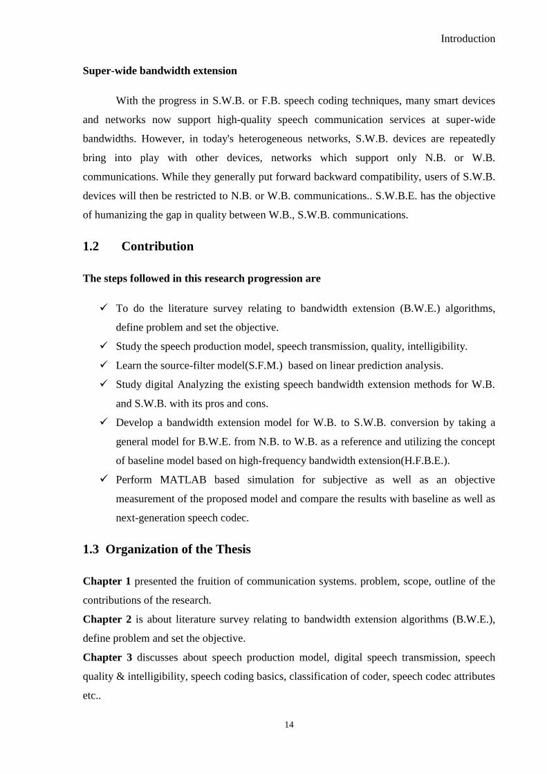
Super-wide bandwidth extension
With the progress in S.W.B. or F.B. speech coding techniques, many smart devices
and networks now support high-quality speech communication services at super-wide
bandwidths. However, in today's heterogeneous networks, S.W.B. devices are repeatedly
bring into play with other devices, networks which support only N.B. or W.B.
communications. While they generally put forward backward compatibility, users of S.W.B.
devices will then be restricted to N.B. or W.B. communications.. S.W.B.E. has the objective
of humanizing the gap in quality between W.B., S.W.B. communications.
1.2 Contribution
The steps followed in this research progression are
To do the literature survey relating to bandwidth extension (B.W.E.) algorithms,
define problem and set the objective.
Study the speech production model, speech transmission, quality, intelligibility.
Learn the source-filter model(S.F.M.) based on linear prediction analysis.
Study digital Analyzing the existing speech bandwidth extension methods for W.B.
and S.W.B. with its pros and cons.
Develop a bandwidth extension model for W.B. to S.W.B. conversion by taking a
general model for B.W.E. from N.B. to W.B. as a reference and utilizing the concept
of baseline model based on high-frequency bandwidth extension(H.F.B.E.).
Perform MATLAB based simulation for subjective as well as an objective
measurement of the proposed model and compare the results with baseline as well as
next-generation speech codec.
1.3 Organization of the Thesis
Chapter 1 presented the fruition of communication systems. problem, scope, outline of the
contributions of the research.
Chapter 2 is about literature survey relating to bandwidth extension algorithms (B.W.E.),
define problem and set the objective.
Chapter 3 discusses about speech production model, digital speech transmission, speech
quality & intelligibility, speech coding basics, classification of coder, speech codec attributes
etc..
Page 41
Organization of the Thesis
15
Chapter 4 talks about the development of the B.W.E. model for W.B. to S.W.B. conversion
by taking detailed analysis of N.B. to W.B. model and reference Algorithm.
Chapter 5 analyses about linear prediction analysis, synthesis with stability criteria.
Chapter 6 discusses MATLAB based simulation for subjective as well as an objective
measurement of the proposed model and compare the results with baseline as well as next-
generation speech codec.
Chapter 7 concluded with overall results and highlights the scope for future work in this
area of research.
Chapter 8 presents a summary of the list of publications and references.
Page 42
Literature Review and Objective of Work
16
CHAPTER-2
Literature Review and Objective of Work
2.1 Literature reviews of different papers
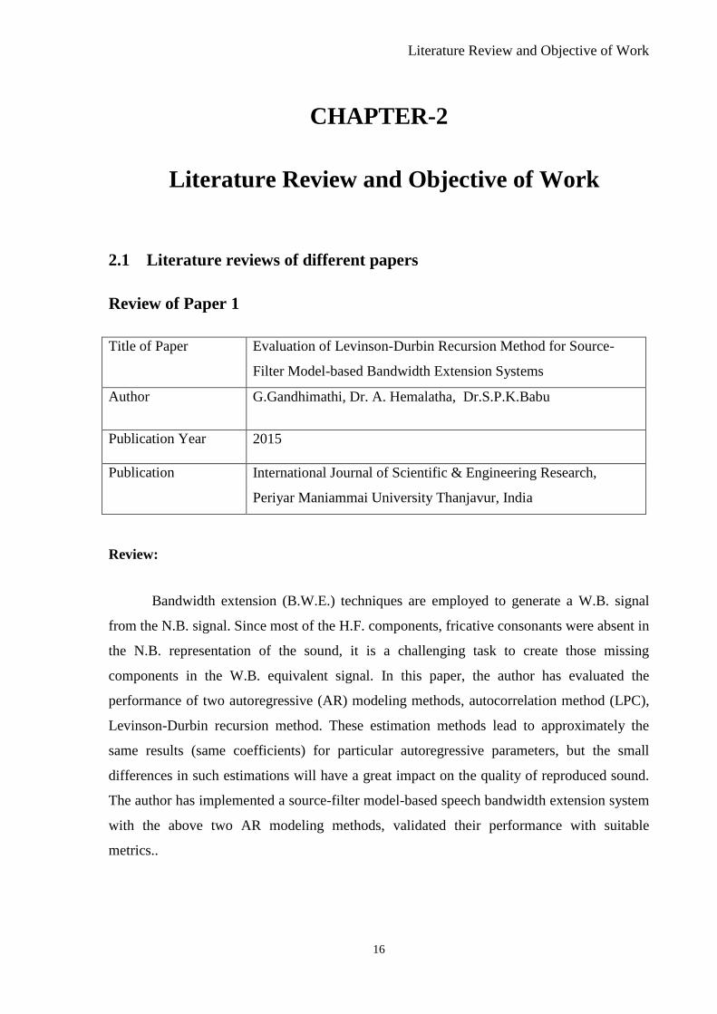
Review of Paper 1
Title of Paper
Evaluation of Levinson-Durbin Recursion Method for Source-
Filter Model-based Bandwidth Extension Systems
Author
G.Gandhimathi, Dr. A. Hemalatha, Dr.S.P.K.Babu
Publication Year
2015
Publication
International Journal of Scientific & Engineering Research,
Periyar Maniammai University Thanjavur, India
Review:
Bandwidth extension (B.W.E.) techniques are employed to generate a W.B. signal
from the N.B. signal. Since most of the H.F. components, fricative consonants were absent in
the N.B. representation of the sound, it is a challenging task to create those missing
components in the W.B. equivalent signal. In this paper, the author has evaluated the
performance of two autoregressive (AR) modeling methods, autocorrelation method (LPC),
Levinson-Durbin recursion method. These estimation methods lead to approximately the
same results (same coefficients) for particular autoregressive parameters, but the small
differences in such estimations will have a great impact on the quality of reproduced sound.
The author has implemented a source-filter model-based speech bandwidth extension system
with the above two AR modeling methods, validated their performance with suitable
metrics..
Page 43
Literature reviews of different papers
17
Review of Paper 2
Title of Paper
Bandwidth Extension for Speech in the 3GPP EVS Codec
Author
Venkatraman Atti ,Venkatesh Krishnan, Duminda Dewasurendra,
Venkata Chebiyyam
Publication Year
2015
Publication
IEEE International Conference on Acoustics, Speech and Signal
Processing (ICASSP)
Review:
In this paper, the author has approached the time-domain bandwidth extension
(T.B.E.) structure employed to code W.B., S.W.B. speech in the newly standardized 3GPP
enhanced voice service codec (E.V.S.). In particular, the advanced modeling techniques used
to recreate the W.B., S.W.B. frequencies with a fewer number of bits paved the way for EVS
to become the most advanced feature-rich conversational speech coder of its time. At 13.2
kbps, the S.W.B. coding of speech uses as low as 1.55 kbps for encoding the spectral content
from 6.4-14.4 kHz. Extensive MOS testing as per ITU-T P.800 has proven that the EVS
codec with time-domain bandwidth extension outperforms in comparisons with all other
standard codec references with significant margins, making it the ideal codec to be deployed
in modern VoLTE networks and other VOIP networks such as VoWiFi.
Review of Paper 3
Title of Paper
Simulation and overall comparative evaluation of performance
between different techniques for high band feature extraction based
on bandwidth extension
Author
Ninad S. Bhatt
Publication Year
2016
Publication
Springer, Int. Journal of Speech Technology
Page 44
Literature Review and Objective of Work
18
Review:
In this paper the author inspect, study, simulate calculation of the High band (H.B.)
component based on linear predictive coding (L.P.C.), M.F.C.C. techniques. The author has
made comparisons of B.W.E. using LPC, MFCC technique for different extension of
excitation. From the simulation result, bar chart for mean opinion score (MOS), Perceptual
evaluation of speech quality (P.E.S.Q.) highlighted by the author in the paper it is clear that
amongst various excitation methods the results obtained for sinusoidal transform
coding(S.T.C.) [82], Full-wave rectification (F.W.R.) as a Non-linear Distortion (N.L.D.)
component produce good results in comparisons with all other techniques for various speech
files for LPC, MFCC based methods[26].
Review of Paper 4
Title of Paper
Audio Bandwidth Extension
Author
Somesh Ganesh
Publication Year
2016
Publication
Georgia Institute of Technology Atlanta, Georgia
Review:
In this paper, the author has provided evidence that the audio bandwidth extension is
a technique used to improve the perceived quality of band-limited audio generated using
various audio codecs. The author proposes a few methods for audio bandwidth extension and
evaluates them by performing listening tests. A comparison between half-wave rectification,
full-wave rectification, along with the use of sub-band filtering is done. The wrapping up
from the experiment conducted is that half-wave rectification performs better than full-wave
rectification as a non-linear device and use of sub-band filtering improves the amount of the
perceived quality in the acquired bandwidth extended output signal.
Page 45
Literature reviews of different papers
19
Review of Paper 5
Title of paper B.W.E. of Speech Signals using Quadrature Mirror Filter
Author
Janki Patel, Nikunj V. Tahilramani and N.S.Bhatt
Publication Year
2018
Publication
IEEE- International Conference on Computation of Power,
Energy, Information and Communication (ICCPEIC)
Review:
In ordinary telephone networks, the speech signal looks like stiffened, muffled, thin
due to limited N.B. frequency range (300 Hz to 3.4 kHz). So it is a prime requirement to
apply the bandwidth extension algorithm on it. Here QMF based B.W.E. system is proposed
which analyzes, synthesizes the speech (voice) signal to acquire W.B. speech (voice) signal
at the receiver side to improve the quality and naturalness of the speech (voice). By applying
the B.W.E. algorithm, the missing higher frequency components of speech can be added at
the end terminal to produce W.B. speech. The objective, subjective evaluations show that the
quality of speech synthesized by the proposed method is better than N.B. speech.
Review of Paper 6
Title of Paper
Super Wideband Spectral Envelope Modeling for Speech Coding
Author
Guillaume Fuchs, Chamran Ashour
Publication Year
2019
Publication
INTERSPEECH 2019, September 15–19, 2019, Graz, Austria,
Erlangen, Germany,
Review:
N.B. speech traditionally transmitted in communication, has been extended to W.B.
(W.B. up to 8 kHz) in digital communications by different standards [83-85]. This trend
continued with the more recent introduction of super-wideband (S.W.B. up to 16 kHz)
speech coders [86-87]. Nonetheless, existing S.W.B. coding solutions are all built on a dual-
band system, coding the lower band separately from the upper band according to a source-
Page 46
Literature Review and Objective of Work
20
filter model of speech production, pure perceptual considerations using a parametric
representation respectively. The spectral envelope is generally modeled in speech coding by
Linear Predictive Coding (LPC) parameters characterizing the vocal tract and acting as an
autoregressive estimation of the speech. Although applying LPC to N.B. and W.B. speech
(voice) is well studied in the literature [88], very little consideration has been given in the
past to the S.W.B. The widening of the audio B.W. has two major impacts on the design of
LPC; the order of the prediction, design of the high-frequency pre-emphasis filter usually
applies before the linear prediction analysis. As the number of samples increases with a
higher sampling frequency, the prediction order must be adjusted accordingly. The LPC
order of 10 usually adopted for N.B. was increased to 16 for W.B. and should probably be
even higher for S.W.B.. However, the order has a significant impact on the bit-rate required
for transmitting the LPC coefficients.
2.2 Review sheet for each paper
Table 2.1 Review summary of all research paper.
Sr.
No
Paper Title
Review:
comment
(include work was done)
1 Evaluation of Levinson-
Durbin Recursion Method
for Source-Filter Model-
based Bandwidth Extension
Systems
1. Source-filter model-based B.W.E. using LPC
coefficients is a simple, reliable technique to achieve
B.W.E. from N.B. to W.B. and it can make a pedestal
for B.W.E. from W.B. to S.W.B.
2. From the Spectrogram comparison of N.B.,
Extended W.B. output by B.W.E., one can note that the
proposed algorithm can able to represent consonant
sounds, mostly fricative consonants like ( th /, sh/, / Isl
/, xl/ ch, /, etc..).
2 Bandwidth Extension for
Speech in the 3GPP EVS
Codec
1. At 13.2 kbps, the super-wideband coding of speech
(voice) uses as low as 1.55 kbps for encoding the
spectral content from 6.4-14.4 kHz.
2. Subjective (MOS) testing as per ITU-T P.800 has
Page 47
Literature reviews of different papers
21
confirmed that the EVS codec with time-domain
B.W.E. performs well in comparison with all other
standard codec references, making it the ideal codec to
be deployed in modern VoLTE & VOIP network.
3
Simulation and overall
comparative evaluation of
performance between
different techniques for high
band feature extraction
based on bandwidth
extension
1. The method employed in this paper is a narrative
approach to inspect, study, simulate calculation of the
High band (H.B.) component based on linear predictive
coding(L.P.C.), Mel frequency cepstral coefficient
techniques.
2. Amongst various excitation methods the results
obtained for sinusoidal transform coding(S.T.C.), Full-
wave rectification (F.W.R.) as a Nonlinear Distortion
component produce good results in comparisons with
all other techniques in terms MOS score for various
speech files for LPC and MFCC based methods.
4 Audio Bandwidth Extension 1. Audio bandwidth extension is a technique used to
improve the perceived quality of band-limited audio
generated using various audio codec.
2. From the conducted listening test as per ITU-T
recommendation for various methods of bandwidth
extension, one can make a note that half-wave
rectification performs better than full-wave
rectification as a non-linear device. The use of sub-
band filtering improves the amount of the perceived
quality in the bandwidth extended signal.
5 Bandwidth Extension of
Speech Signals using
Quadrature Mirror Filter
1. QMF based B.W.E. system analyzes and synthesizes
the speech (voice) signal to acquire W.B. speech
(voice) signal at the receiver side to improve the
quality, naturalness of the speech (voice).
2.The missing higher frequency components of speech
(voice) can be added at the end terminal to produce
W.B. speech (voice).
3.The objective, subjective evaluations show that the
Page 48
Literature Review and Objective of Work
22
quality of speech (voice) synthesized by the proposed
method is better than N.B. speech.
6 Super Wideband Spectral
Envelope Modeling for
Speech Coding
1.The author is paying attention to the spectral
envelope modeling by Linear Predictive Coding (LPC)
parameters characterizing the vocal tract.
2. The order of the prediction, design of the high-
frequency pre-emphasis filter usually applied before
the linear prediction analysis.
3. As the number of samples increases with a higher
sampling frequency, the prediction order must be
adjusted accordingly. The LPC order of 10 usually
adopted for N.B. was increased to 16 for W.B. and
should probably be even higher for SW.B.
4. The order has a significant impact on the bit-rate
required for transmitting the LPC coefficients.
2.3 Summary of Literature Survey
Bandwidth extension algorithms (B.W.E.) aspire to estimate missing higher
frequency components at 3.4-8kHz for W.B. or 6.8-16kHz for S.W.B. signal. In this chapter,
a survey of approaches to B.W.E. is presented. While B.W.E. approaches focus on N.B. to
W.B. extension, S.W.B.E. approaches for W.B. to S.W.B. extension are developed to bridge
the quality gap between W.B., S.W.B. communication. While studying bandwidth extension
several parameters, constraints need to be taken into consideration to propose a highly
efficient algorithm that introduces only negligible latency. During the literature review many
research papers, websites, journals, other articles on wireless-communication [1-5], [10],
ETSI standard [14],[17],[19], ITU-T Recommendation [8],[9],[12],[18],[22-23]
[25],[27],[29],[33],[109],[137-138],[140],[145], 3GPP TS series [20],[38],[40],[41],[59] for
coding of speech followed by B.W.E. [6],[34],[35],[54],[55],[62],[64],[65],[67],[77] are
referred. A general overview of the bandwidth extension has been presented in many
research papers [7],[13],[45-46],[50-52],[68][81]. This step led us to define the research
problem. In [69] author has given a solution to trim down the wideband speech coder bit-rate
Page 49
Summary of Literature Survey
23
by coding the parameters of wideband voice (speech) employing noteworthy enlarge in bit-
rates of N.B. coders. [51-52],[70-71] have discussed various approaches (i.e..Linear
Prediction algorithm using L.P.C. coefficients, codebook mapping approach) and make
subjective measurement comparison for various audio wave files.
Performance assessment of speech (voice) signal based on the sub-band filter
followed by source-filter model are discussed in [72]. Based on review it is found that Linear
prediction is an effective tool for the bandwidth extension. It plays a very significant role in
achieving data rate compression. After studying detailed linear prediction analysis, synthesis,
stability criteria, it is found that for next-generation wireless communication bandwidth
extension from the signal itself (without sending sideband information) is useful for data rate
reduction because no need of sending information in sideband is needed for reproduction of
signal at the receiver side. Codebooks mapping [73-74], linear mapping [75], Neural
Networks, etc.. are used to estimate the missing components. [76-78] bring into being the
potential features of speech (voice), evaluate their performance for BWE application. In [79]
author is paying attention to various approaches for bandwidth extension namely with and
without speech (voice) production model as well as BWE with side information. The author
has listed out all the techniques of estimation of the wideband spectral envelope. In [80] the
author has designed the source-filter model based on the vocal tract to retrieve bandwidth
extended output. So in this thesis, the basic discussion that takes place here is between first
general model and baseline model. Based on that model proposed system model for B.W.E.
with flow diagram are discussed. Simulation results achieved for proposed system model in
terms of mean opinion score (M.O.S.), perceptual evaluation of speech quality (P.E.S.Q.),
spectrogram are compared with baseline algorithm, next-generation super wideband coder
algorithm.
2.4 Definition of the Problem
The problem title is " Analytical Studies Relating To Bandwidth Extension of Speech
Signal For Next Generation Wireless Communication". The problem is the B.W.E. of the
speech (voice) signal from W.B. to S.W.B. to improve naturalness, pleasantness, clarity, the
brightness of the speech (voice) signal. In next-generation wireless communication many
smart devices hold up high-quality speech (voice) communication services at S.W.B. so
B.W.E. play a important role for the system.
This can be done by:
Page 50
Literature Review and Objective of Work
24
Employing S.F.M. based approach by taking general model for B.W.E., baseline
algorithm as a reference to achieve B.W.E. from W.B. to S.W.B. In the approach
performance of the subjective listening test (MOS) as per ITU-T recommendation for various
speech (voice) files followed by comparisons of spectrogram of estimated S.W.B. with the
baseline algorithm & next-generation super wideband coder algorithm is carried out.
2.5 Objectives and Overview of the Research
Bandwidth extension (B.W.E.) is utilized to produce W.B. & S.W.B. as good as
voice quality at end devices without much modification in the existing environment. In other
words, one can say that the objective of bandwidth extension (B.W.E.) is to extend the
bandwidth (B.W.) of the reproduced sound by synthesizing, adding additional high-
frequency components to the received low-band width speech signal.
So the objectives of bandwidth extension(B.W.E.) are listed as follows.
To increase transparency and genuineness of recovered speech, N.B.→W.B.
Further improvement in transparency and genuineness of speech (voice) signal,
W.B.→S.W.B.
To propose an algorithm based on the source-filter model(S.F.M.) by taking a baseline
algorithm as a reference and compare it with next-generation super wideband coder in terms
of perceptual evaluation of speech quality (PESQ), mean opinion score (MOS),
complementary mean opinion score (CMOS).
Compare the spectrogram of the extended output of baseline coder, proposed coder, next-
generation S.W.B. coder and prove that results obtained based on the proposed coder are
comparable with baseline as well as a next-generation super wideband coder.
B.W.E. based on the source-filter model is a suitable choice because the illustration of
20ms (frame duration) * 8KHz (sampling frequency) -160 samples by just 12 (twelve)
parameter results in data rate reduction ultimately save the bandwidth and storage
requirements.
The digital filter and its slowly changing parameters are the key factors to achieve
compression of a speech signal.
The research work presented here can be utilized to get better speech (voice) quality
obtainable by the W.B. system and to conserve speech (voice) quality when S.W.B. devices
are used at the side of W.B. services.
Page 51
Introduction
25
CHAPTER-3
Fundamental of Speech Production Model,
Types of Speech coder and its attributes
3.1 Introduction
Before studying in detail regarding B.W.E. for next-generation wireless
communication, it is essential to know the fundamental of the speech (voice) production
process as well as the data rate of a speech (voice) signal. A speech (voice) signal is defined
as the acoustic wave that is radiated from the human speech production arrangement when
air is expelled from the lungs, resulting flow of air is agitated by a constriction someplace in
the vocal tract.
Fig.3.1 represents speech (voice) production system model. A speech (voice) signal
is created by a speaker at his/her mouth or lips in the form of pressure waves. The organs
engaged in the speech (voice) creation mechanism are the lungs, larynx, vocal tract (V.T.).
The lungs generated an airflow is modulated by vocal cords or vocal folds of the larynx. The
airflow passing through the glottis-a slit-like orifice between the two vocal folds–is
translated to either a quasi-periodic or noisy airflow by the vocal folds vibration. The
resulting airflow source stimulates the V.T. that comprises oral, nasal, pharynx cavities. The
V.T. performs spectral shaping or coloring of the excitation source. The subsequent variation
of air pressure at the lips is spread out in the form of traveling waves called speech (voice)
[90]. Speech (voice) signals can be seen as the output of a filtering operation in which the
V.T. system (or filter) is excited by the modulation of an excitation source or airflow. The
mechanism is typically known as the source-filter model (S.F.M.) of speech (voice)
production which allows the modeling of speech (voice) signals as a convolution of the
impulse response of the V.T. filter, excitation source [91].
This section presents a concise overview of the different speech (voice) sounds with
their spectral characteristics, B.W. limitations imposed by telephone filter etc..
Page 52
Fundamental of Speech Production Model,
Types of Speech coder and its attributes
26
Figure 3.1 Speech (voice) production system model [90]
This section provides a brief overview of different speech sounds, their spectral
characteristics, bandwidth limitations imposed by telephone filter results in terms of
intelligibility,quality.
3.2 Speech (voice) sounds
Speech (voice) sounds are extensively separated into two categories: vowels, consonants
[147].
Vowels:
Vowels form the largest group of phonemes. The characteristics of vowels change based on
the position of the tongue–that mainly determine the V.T. shape – towards the front, center,
or back of the oral cavity [147].
Consonants:
Consonants form the second largest group of phonemes. It can be subcategorized into
nasals, plosives, fricatives, whispers, affricates [147].
Page 53
Speech (voice) sounds
27
Nasals:
Nasals are closest to vowels, produced at the nostrils by the quasi-periodic airflow only
through the nasal cavity; the oral cavity remains constricted. Depending upon the place of
constriction that is formed by the tongue across the oral cavity, nasals are distinguished, e.g.
/m/ as in “mo” and /n/ as in “no”[147].
Fricatives are of two types.
Unvoiced fricatives:
Unvoiced fricatives (e.g., /sh/ in “should”) are described by a noise source generated
due to turbulent airflow near the V.T. constriction. The noise source is spectrally shaped
depending upon the location, degree of constriction formed by the tongue at the teeth or lips
or along the oral cavity [147].
Voiced fricatives:
Voiced fricatives (e.g. /z/ as in “zebra”) are generated by the concurrent generation of
noise at the constriction, vibration of the vocal folds. These sounds are formed by a
combination of a noisy, periodic airflow [147].
Diphthongs:
Diphthongs are produced by vibrating vocal folds analogous to vowels, however, the
V.T. does not remain steady, but varies smoothly between two vowel configurations. So
diphthongs are described by formant transitions as the V.T. articulation changes gradually
between two vowel positions. The examples of diphthongs are /Y/ as in "hide", /W/ as in
"out", /O/ as in "boy" and /JU/ as in "new[147].
Spectral characteristics of speech sounds:
Different speech (voice) sounds are distinguished by different temporal, spectral
characteristics. it can be distinguished from each other based upon their acoustic properties
like rapid transitions in spectral content, abrupt changes in amplitude, presence or lack or
combination of voicing, spectral shape attributed to the V.T. configuration [92]. Based on
spectral properties, speech (voice) sounds can be categorized into voiced, unvoiced sounds
[147].
Page 54
Fundamental of Speech Production Model,
Types of Speech coder and its attributes
28
Voiced sounds:
The voiced sounds are the end result of excitation of the V.T. by a quasi-periodic
glottal airflow. They are expressed by a quasi-periodic time-domain waveform with large
variations in magnitude. The periodicity is calculated in terms of the pitch period. The
magnitude spectra of voiced sounds thus exhibit harmonic structure with peaks at integer
multiples of the fundamental frequency or pitch, especially in the L.F. region. [7,91].
Unvoiced sounds:
Unvoiced sounds are differentiated by time-domain waveforms with relatively lower
magnitude than voiced sounds, however, with rapid variations as a result of the noise-like
nature of the excitation source. So, the spectrum of unvoiced speech broadens over the whole
audio spectrum [147].
3.3 Representation of Speech Signals
There are many possibilities for the discrete-time representation of speech (voice)
signals as shown in fig.3.2. These representations can be classified into two broad groups,
namely waveform representation, and parametric representations.
Waveform representations are concerned with simply preserving the “wave shape” of
analog speech (voice) signal through a sampling, quantization process. Parametric
representations are concerned with representing the speech (voice) signal as the output of a
model for the speech (voice) production. The first step in acquiring a parametric
representation is often a digital waveform representation; (speech (voice) signal is sampled,
quantized and then further processed to achieve the parameters of the model for speech
(voice) production). The parameters of the models are classified as either excitation
parameters (it is related to the source of speech (voice) sounds or vocal tract response
parameters) [146].
3.4 Classification of Coder
In past for landline communication PCM-64kbps was used. After that ADPCM-
32kbps was used to enlarge the speech (voice) channel by a factor of 2. LPC based source
coders are become popular in the world market which is good for estimating basic speech
parameters like pitch, formant, V.T. area function, etc.. It is used for representing speech
Page 55
Classification of Coder
29
(voice) for low bit rate transmission or storage It requires 80000 bits for 100s speech frame
which is less than PCM-6400000 and ADPCM-3200000 bits.
The hierarchy of speech (voice) coder is shown in fig. 3.3. Speech coders differ
widely in their approaches to achieving signal compression. Based on how they accomplish
compression, speech (voice) coders are broadly classified into two categories: waveform
coders, vocoders. Also, there exists a hybrid coder made up of a combination of both the
coder to provide a good quality speech (voice) at low bit rates. The speech (voice) quality
produced by speech (voice) codec is a function of transmission bit-rate, complexity, Delay,
bandwidth. Hence when considering speech (voice) codec it is essential to consider all these
attributes [146].
3.4.1 Waveform Coding
Waveform coding techniques were the first to be investigated and are still widely
embodied in the relevant standards. In this class of coding, the objective is to minimize a
criterion that measures the dissimilarity between the original, reconstructed speech (voice)
signals, evaluated on a block-by-block basis. A block can be as small as one sample [146].
Waveform codec attempt, without using any knowledge of how the signal to be
coded was generated. Results from such codec can be improved if the predictor and
Representation
speech signals
Waveform
Representation
Parametric
Representations
Exercitation
Parameters
Vocal tract
Parameters
Figure 3.1
Figure 3.2 Representation of speech (voice) signals
Page 56
Fundamental of Speech Production Model,
Types of Speech coder and its attributes
30
quantizer are made adaptive so that they change to match the characteristics of the speech
(voice) being coded. This leads to Adaptive Differential PCM (ADPCM) codec.
Figure 3.3 Hierarchy of speech coders[146]
Waveform coders are most useful in applications that require the successful coding of
both speech, no speech signals. In the public switched telephone network (PSTN) successful
transmission of modem, fax signaling tones, switching signals is nearly as important as the
successful transmission of speech (voice). The most commonly used waveform coding
algorithms are uniform 16-bit PCM, commanded 8-bit PCM, ADPCM [146].
3.4.2 Source Coding
Source coders operate using a model of how the source was generated, attempt to
extract, from the signal being coded, the parameters of the model which are transmitted to
the decoder. The V.T. is represented as a time-varying filter, excited with either a white
noise source, for unvoiced speech segments, or a train of pulses separated by the pitch period
for voiced speech (voice). Therefore the information which must be sent to the decoder is the
filter specification, a voiced/unvoiced flag, the necessary variance of the excitation signal,
Page 57
Classification of Coder
31
pitch period for voiced speech. This is updated every 10-20 ms to follow the non-stationary
nature of speech (voice).
The model parameters can be determined by the encoder in several different ways,
using either time or frequency domain techniques. Also, the information can be coded for
transmission in various ways. Vocoders tend to operate at around 2.4 kbit/s or below,
produce speech (voice) which although intelligible is far from natural sounding. Increasing
the bit rate much beyond 2.4 kbit/s is not worthwhile because of the inbuilt limitation in the
coder's performance due to the simplified model of speech (voice) production used. The
main use of vocoders has been in military applications where natural-sounding speech
(voice) is not as important as a very low bit rate to allow heavy protection, encryption [146].
3.4.3 Hybrid Coding
Waveform coders are capable of providing good quality speech (voice) at bit rates
down to about 16 kbit/s but are of limited use at rates below this. Vocoders on the other hand
can afford an intelligible speech (voice) at 2.4 kbit/s and below, but cannot provide a natural-
sounding speech (voice) at any bit rate.
A hybrid coder tends to act like a waveform coder for high bit-rate, parametric coder
at low bit-rate, with fair to good quality for medium bit-rate. This technique dominates the
medium bit-rate coders. The most successful, commonly used coder are time-domain
Analysis-by-Synthesis (ABS) codec. Such coders use the same linear prediction filter model
of the vocal tract as found in LPC vocoders. However, instead of applying a simple two-
state, voiced/unvoiced, model to find the necessary input to this filter, the excitation signal is
chosen by attempting to match the reconstructed speech waveform as closely as possible to
the original speech (voice) waveform [146].
3.5 Speech (voice) coding
Speech (voice) coding algorithms have the target of approximating the compact
digital representations of continuous speech (voice) signals for efficient storage, transmission
[94]. In the year 1990s, the increased number of mobile phones, demands to mobile
communications brought new challenges for digital speech transmission systems [7]. General
block diagram of speech coding is shown in fig. 3.4.. As represented in the diagram the
digital transmission of speech (voice) involves A to D converter to covert continuous data in
digital arrangement. The function of codec at the encoder side is to converts an continuous
Page 58
Fundamental of Speech Production Model,
Types of Speech coder and its attributes
32
signal into squeezed, binary bits pattern as indicated in fig. 3.4. This binary bits pattern can
be sent over digital wireless networks. At the recipient side, the binary bit stream is
translated back to an continuous signal using a decoder. Codec are utilized in telephones,
cellular networks, televisions, set-top boxes etc..[89].
Considering the speech (voice) codec attributes like low complexity, limited delay,
lower cost, limited radio network resources it is must be necessary to operate speech (voice)
codec at lower bit rate [93,95]. Perception plays a fundamental role in the art of lossy speech
(voice) coding. Lossy speech (voice) coding can be summarized as the endeavor to reduce
the bit rate of the coded speech (voice) through an efficient, minimal representation of the
speech (voice) signal while maintaining an acceptable level of perceived quality of the
decoded speech (voice).
Fig. 3.5 (a) and 3.5 (b) show a section of the spectrogram for an unvoiced and a
voiced sound respectively. The range from 300-3400 Hz is called the narrowband. The
complete range is referred to as wideband. The "missing" range in narrowband compared to
the wideband is referred to as the extension band. Throughout the thesis the bands will
frequently be referred to by their abbreviations; N.B., W.B.,E.B. respectively. As can be seen
in both cases, there is a considerable amount of energy in the extension band, which would
result in a significantly improved version of the speech (voice)[69].
Speech can be divided into two classes, voiced and unvoiced. The difference between
the two signals is the use of the vocal cords and V.T. (mouth and lips). When voiced sounds
are pronounced you use the vocal cords, vocal tract. Because of the vocal cords, it is possible
to find the fundamental frequency of the speech. In contrast to this, the vocal cords are not
Speech
Encoder
Transmission Speech
Decoder
Transmitter Channel Receiver
Discrete Sample s (n)
10110011…..., 64kbps
1001..,
8kbps
1001…,
8kbps
10110011…,
64kbps
D/A
Converter
Retrieved
speech s^ (t)
A/D
Converter
Analog
speech s(t)
Figure 3.4 General block diagram of speech coding
Page 59
Speech (voice) coding
33
used when pronouncing unvoiced sounds. Because the vocal cords are not used, is it not
possible to find a fundamental frequency in unvoiced speech. In general, all vowels are
voiced sounds. Examples of unvoiced sounds are /sh/ /s/ and /p/.There are different ways to
detect if voices are voiced or unvoiced. the fundamental frequency can be used to detect the
voiced and unvoiced parts of speech. Another way is to calculate the energy in the signal
(signal frame). There is more energy in a voiced sound than in an unvoiced sound [69].
Figure 3.5 Voice (a) and Unvoiced (b) Speech frame representation [69]
3.6 Issues related to digital speech coding
Digital coding of speech (voice), bit rate reduction process has thus emerged as an
important area of research. This research largely addresses the following problems:
Although it is very attractive to reduce the PCM bit rate as much as possible, it
becomes increasingly difficult to maintain acceptable speech (voice) quality as the bit
rate falls.
As the bit rate falls, acceptable speech (voice) quality can only be maintained by
employing very complex algorithms, which are difficult to implement in real-time
even with new fast processors with their associated high cost, power consumption, or
by incurring excessive delay, which may create echo control problems in system.
Page 60
Fundamental of Speech Production Model,
Types of Speech coder and its attributes
34
To achieve low bit rates, parameters of speech production and/or perception model
are encoded and transmitted [96].
Speech quality as produced by speech codec is a function of transmission bit rate,
complexity, delay, B.W.. Therefore when considering speech (voice) codec it is essential to
consider all these attributes. For a given application some attributes are predetermined while
trade-off can be made among others. For example, low bit rate speech codec tends to have
more delay as compared to the higher-bit-rate codec. They are generally more complex to
implement, often have lower speech quality than the higher-bit-rate codec [146].
3.7 Speech codec attributes
Speech codes are characterized by five general attributes:-
3.7.1 Transmission bit rate
Specification of how many bits are required to describe one second of speech. The bit
rate is a measure of how much the speech model has been exploited in the coder; the lower
the bit rate, the greater the reliability on the speech production model. Depending on the
system and design constraints, fixed-rate or variable-rate speech coders can be used [146].
3.7.2 Speech Quality
The speech quality has the most important dimensions among all the attributes. The
decoded speech should have a quality acceptable for the target application. Bit rate, quality
are intimately related: the lower the bit rate, the lower the quality. While the bit rate is
inherently a number, it is difficult to quantify. The most widely used subjective measure of
quality is the Mean Opinion Score (MOS), which is the result of averaging opinion scores
for a set of untrained subjects (listeners). Each listener characterizes each set of utterances
with a score on a scale from 1 to 5 (1-bad, 2-poor, 3-fair, 4-good, 5- excellent). The MOS
quality rating is shown in Table 3.1. A MOS of 4.0 or higher defines good or toll-quality,
where the reconstructed speech (voice) signal is generally indistinguishable from the original
signal. A MOS between 3.5 and 4.0 defines communication quality, which is sufficient for
telephone communications. The most widely used objective measure of quality is the signal-
to-noise- ratio (SNR), SNR indicates how well the waveforms match but do not account for
how the decoded speech (voice) is perceived [146].
Page 61
Issues related to digital speech coding
35
Table 3.1 MOS Quality Rating
Quality scale Score Listening effort scale Impairment
Excellent 5 No effort required Imperceptible
Good 4 No appreciable effort
required
Perceptible but not
annoying
Fair 3 Moderate effort required Slightly annoying
poor 2 Considerable effort
required
Annoying
bad 1 No meaning understood
with reasonable effort
Very annoying
3.7.3 Bandwidth
The B.W. of the speech signal that needs to be encoded is also an issue. Typical
telephony requires 200–3400 Hz B.W. Wideband speech coding techniques (useful for audio
transmission, teleconferencing, tale teaching) necessitate 7–20 kHz bandwidth [146].
3.7.4. Communication Delay
The measure of the time taken for an input sample to be processed at the encoder,
transmitted, and decoded at the decoder. Delays over 150 ms can be unacceptable for highly
interactive conversations. Coder delay is the sum of different types of delay. The first is the
algorithmic delay arising because speech coders usually operate on a block of samples
(frames), which needs to be accumulated before processing can begin. The computational
delay is the time that the speech (voice) coder acquires to course of action the frame. In
practice, the total delay of many speech coders is at least three frames[146].
3.7.5 Complexity
Complexity is defined as The measure of computation (memory) required to
implement the coder. The computational complexity, memory requirements of a speech
(voice) coder determine the cost, power consumption of the hardware on which it is
implemented. In most cases, the real-time operation is required at least for the decoder. A
large complexity can result in high power consumption in the hardware [146].
Page 62
Fundamental of Speech Production Model,
Types of Speech coder and its attributes
36
3.8 Speech codec for next-generation wireless communications
Selection of Particular speech (voice) codec plays a vital role in design of digital
next-generation wireless communications. it a challenging task to shrink speech (voice) to
maximize the number of user on the system. The other important parameters are encoding
delay, complexity in design of encoder, necessity of power requirement, compatibility with
on hand standards, robustness of the coded speech (voice) to transmission errors etc...[146].
3.9 Speech (voice) quality, intelligibility
In a telephone chat, the acoustic signal is recognized by the near-end user's ear, origin
an auditory event in the brain results in a depiction of the voice (sound) [96]. former
knowledge of the communication system, emotions of the listener influence the quality
judgment [13,97]. According to [98] speech (voice) quality encompasses attributes such as
naturalness, clarity, pleasantness, brightness. Intelligibility is considered as a other
dimension to measure speech (voice) quality [7]. Besides the traditional N.B. (300–3.4kHz)
speech coding, transmission, W.B. (50–7kHz), S.W.B. (50–14kHz) speech transmission has
been deployed in many telephone applications..
3.9.1 Listening-only tests
Listening-only tests can play a vital role in assessing speech (voice) quality of a
communication system. This test can be done by means of pre-recorded, processed set of
speech (voice) samples (through headphones). The subjects are requested to assess the
quality using a predefined scale given by the experimenter. An advantage of listening-only
tests is that the evaluation is subjective, i.e. subjects listen to real speech samples, grade them
according to their personal opinion. A drawback listening-only tests is that test design
factors, rating procedures affect the subject's observation procedure. As shown in table 3.2.,
subjects are asked to assess the speech (voice) quality using the 5-point mean opinion scale
(MOS) for absolute category rating (ACR) test [99]. In degradation category rating (DCR)
test the subject is asked to assess a degraded signal w.r.t. reference signal using the
degradation mean opinion score (DMOS) as shown in table 3.3.
Page 63
Speech codec for next-generation wireless communications
37
Table 3.2 MOS as per recommendation ITU-T P.800 [99]
Score Quality of speech
5 Excellent
4 Good
3 Fair
2 Poor
1 Bad
Table 3.3 Degradation means opinion score as per recommendation ITU-T P.800 [99]
Score Degradation is
5 Inaudible
4 Audible but not annoying
3 Slightly annoying
2 Annoying
1 Very annoying
In the comparison category rating (CCR) test, two signals are judge against each
other as shown in table 3.4
Table 3.4 Comparison means opinion score according to ITU-T P.800 [99]
Score Quality of the second compared
to that of the first
3 Much better
2 Better
1 Slightly better
0 About the same
-1 Slightly worse
-2 Worse
-3 Much worse
3.9.2 Conversational tests
In comparisons with previous tests, conversational tests are much close to real
conversation situation. The test can be utilized to assess either a specific source of
degradation, such as delay or echo, or the overall quality of a transmission system. In test,
Page 64
Fundamental of Speech Production Model,
Types of Speech coder and its attributes
38
two subjects at a time are situated in separate soundproof rooms. The subjects can be experts,
experienced, or naive participants depending on the rationale of the test. During the test, the
subjects have a dialogue on a given topic or task, give their opinion on the speech (voice)
quality [100].
3.9.3 Field tests
This test is utilized to assess speech (voice) quality of transmission systems in most
realistic environment. For example, the speech (voice) quality of a wireless phone might be
judged during true phone calls. The arrangement of such a test is expensive during system
process development. so quality tests are typically arranged in laboratory.
3.9.4 Intelligibility tests
It is one types of subjective test computed as correctly recognized speech (voice)
sounds at the receiver side of a system in percentage. In rhyme tests rhyming words are
utilized[106]. The diagnostic rhyme test (DRT) consists of 96 rhyming word pairs that differ
in their initial consonant [107]. The modified rhyme test (MRT) contains 50-word lists of six
one-syllable words, differing in either the opening or the closing consonant [108]. To find a
presentation level for test speech (voice) speech reception threshold (SRT) test can be
utilized. In this test it is necessary for a listener to understand the speech (voice) correctly a
specified percentage of the time, usually 50%.
3.10 Objective quality evaluation
Objective quality estimation techniques are computational tools build-up to assess the
quality of speech (voice) signals. Objective quality assessment methods are often classified
into two parts namely parameter based, signal-based models [101-102]. Parameter-based
models, such as E model [103], rate the important quality of a whole transmission path. They
provide information on the whole network, helpful in planning of network. Signal-based
methods play a very important role in speech (voice) enhancement field. The perceptual
evaluation of speech (voice) quality (PESQ), normalized in ITU-T Recommendation P.862
[104], can be employed to assess N.B./W.B/S.W.B. quality. Both the degraded and a
reference signal are required for evaluation of speech (voice) quality. An extension of the
PESQ is presented in the recommendation P.862.2 [105].
Page 65
Speech (voice) quality, intelligibility
39
3.11 Effect of B.W. on speech (voice) quality, intelligibility
Selection of cut-off frequencies, telephone filter characteristics specified in ITU-T
recommendation G.120 [109] was relies on the B.W. limitations obliged by continuous
transmission systems. The selections were motivated by outcomes attained from subjective
listening tests [11]. To retain compatibility with existing analog PSTNs, initial progress in
digital telephony has occurred with B.W. constraints of 0.3-3.4kHz. After digitization of
speech (voice) transmission, speech (voice) coding techniques were developed to condense
speech (voice) signals to lower bit rates than PCM, without degrading speech (voice) quality.
So the bandwidth available for speech (voice) transmission was dictated by development of
cellular systems, speech (voice) coding techniques. However, the frequency content of
speech (voice) signals ranges from 60Hz to 20kHz.
The drawbacks upon the telephone B.W. thus result in a lack of distinctive spectral
properties of speech (voice) sounds. Some fricatives such as /f/ and /s/ differ in the location
of the lowest spectral peak, which occurs typically around 2.5kHz, 4kHz for a male adult
speaker correspondingly. Such distinctive properties are vanished in typical telephone speech
(voice), which often causes difficulties to the listener in distinguishing between different
fricative sounds [15]. Some plosives (/t/ and /d/) are characterized by higher energy bursts
occurring around 3.9kHz. Others (/b/, /p/) also exhibit similar energy bursts albeit with less
intensity. These distinct properties are vanished in N.B. speech (voice) results in trim down
intelligibility, naturalness for plosives. Nasals are too affected. They are dominated by the
first formant F1 which typically occurs around 250Hz. This is also vanished due to the lower
cut-off of the telephone band.
During a telephone call, occasionally H.F. sounds such as /f/ and /s/ (or /p/ and /t/)
are hard to distinguish. Improvements in intelligibility are thus essential to shrink the
listening effort, to afford comfortable communications [6]. The perceived quality as well as
the intelligibility of speech (voice) signals enhancing with increases in acoustic B.W.,
particularly for unvoiced sounds. This is because they restrain a substantial portion of their
spectral content beyond 3.4kHz. A changeover from N.B. to W.B. communication then
obviously leads to an raise in syllable, sentence intelligibility from 90% ,99.3% to 98%,
99.9% correspondingly [110-111]. The quality of communication is further improved at
S.W.B.
Page 66
Development of Bandwidth Extension Model For W.B. To S.W.B.
40
CHAPTER-4
Development of Bandwidth Extension Model
For W.B. To S.W.B.
4.1 Introduction
Before studying in detail regarding development of bandwidth extension model for
W.B. To S.W.B. general model for B.W.E. from N.B. to W.B., bandwidth limitation in
compressed speech/audio, High-Frequency Bandwidth Extension (H.F.B.E.) algorithm [120]
are discussed. The B.W.E. approaches can be categorized into two parts namely Non-model
based B.W.E., source-filter model based B.W.E..
4.2 Non-model based B.W.E. approaches
The non-model based B.W.E. approaches do not use a priori knowledge about speech
(voice) production mechanism and employ simple operations to introduce missing frequency
components. The operations include spectral translation or shifting (fixed or adaptive),
generation of high-frequency components via non-linear operations on time-domain signals,
band pass filtering on white noise, etc. Some approaches also perform spectral shaping of the
generated frequency components using some gain control parameter or an empirically
determined filter. The first commercial use of such B.W.E. methods by the British
Broadcasting Corporation (BBC) [112] is reported in the year 1972 where the acoustical
bandwidth of telephone speech in broadcast programs is improved. The notable examples are
[113-116]. Such methods, however, produce extended W.B. speech (voice) signals with
audible processing artifacts and distortions. This is because the energy of the generated
frequency components is either too weak or too strong compared to the N.B. component
[117]. Additionally, the quality of extended speech (voice) signals depends upon the
effective bandwidth of the original input signal [118].
Page 67
Introduction
41
4.3 B.W.E. approaches based on the source-filter model
The model-based B.W.E. algorithms use a priori knowledge about characteristics of
speech (voice) signals, human speech (voice) production mechanism. Since the beginning of
the 90s, most B.W.E. algorithms started exploiting the classical source-filter model (S.F.M.)
[119] of speech (voice) production where an N.B./W.B. speech signal is represented by an
excitation source, vocal tract filter. The frequency content of these two components can be
extended through independent processing before a W.B./S.W.B. signal is resynthesized.
The extension of N.B./W.B. speech is thus divided into two tasks;
Estimation of H.B. or W.B./S.W.B. spectral envelope from input N.B./W.B. features
via some form of an estimation technique
Generation of H.B. or W.B./S.W.B. excitation components via some form of time-
domain non-linear processing, spectral translation or spectral shifting methods. The
H.B. component is usually parameterized with some form of linear prediction (LP)
coefficients whereas the N.B./W.B.component is parameterized by a variety of static
and/or dynamic features
4.3.1 B.W.E. from N.B. to W.B. Speech Conversion:
In Digital Signal Processing signals are band-limited w.r.t. use of sampling
frequency. N.B., W.B., S.W.B. speech has a sampling frequency of 8kHz,16 kHz,24 kHz
respectively. Based on N.B. to W.B. speech conversion and baseline algorithms (H.F.B.E.)
proposed method for W.B. to S.W.B. has been discussed. It is a blind method because they
estimate missing H.F. component from available L.F. components. The proposed flow chart
of bandwidth extension based on baseline and proposed algorithms discuss the achievement
of W.B./S.W.B. speech signal at the receiver side without actually transmitting W.B./S.W.B.
4.3.2 General Model for B.W.E.:
The fundamental thought adopted here for the B.W.E. system is the separate
extension of the spectral envelope and the residual signal as depicted in fig.4.1. First, the
incoming telephone-band signal is analyzed through the LPC-analysis. Based on the spectral
envelope, telephone-band short time features, the spectral envelope is extended. The
extended version is essential to define the shaping filter characteristic. Second the extended
Page 68
Development of Bandwidth Extension Model For W.B. To S.W.B.
42
residual signal for this shaping filter is calculated from the telephone-band residual signal as
highlighted in fig.4.1. According to the linear speech production model the synthetic signal
is generated by driving the shaping filter with the extended residual signal. The resulting
power of the synthetic signal has to be matched to the telephone-band signal power such that
both signals can be added to build the desired W.B. signal [70].
Figure 4.1 General Model for B.W.E.[70]
4.3.3 Bandwidth Limitation in Compressed Speech/Audio:
Most perceptual speech/audio codec B.W. limits the input signals to use the available
bits for psycho acoustically relevant L.F. signals. The B.W. limitation becomes severe at
very low bit rates e.g. 128kbps mp3 encoded speech/audio is bandwidth limited to about 15
Page 69
B.W.E. approaches based on the source-filter model
43
kHz and 64kbps mp3 to about 8 kHz. Fig. 4.2 shows an example of a 96 kbps mp3 encoded-
decoded signal spectrum, the signal spectrum chopped beyond 11 kHz. These missing H.F.
signals cause speech/audio signals to sound dull and at times muffled. so it is becoming
essential to improve audio quality in such cases by artificially creating high frequencies from
low-frequency information[120].
Figure 4.2 Bandwidth Limitation in Compressed Speech/Audio [120]
Issues with the Approaches:
Bandwidth limitation becomes severe at very low bit rates.
Proposed Solution
Encoder side modifications solve the bandwidth limitation issues.
Internal Issue
An enormous amount of content available which suffers from the above-mentioned
quality issues.
Proposed Solution
Post-processing methods after decoding Ex..spectral extrapolation
Internal Issue
Computationally too expensive
Final Solution-
Employ Time-Domain Method for real-time Implementation.
Page 70
Development of Bandwidth Extension Model For W.B. To S.W.B.
44
4.3.4 Baseline System Model for B.W.E.
As shown in fig.4.3 baseline system model accepts decoded data as input from any
lossy audio decoder and recreates high frequencies blindly i.e. by using only the decoded
audio signal and nothing else. Since the bandwidth of the input signal is unknown it is first
estimated by using a real-time bandwidth detection process. After detecting the highest
frequency present in the signal at any given time, the decoded signal is divided into sub-
bands up to half the detected highest frequency of the signal. Each sub-band signal is then
individually passed through non-linearity to generate harmonics. The generated harmonics
are gain scaled to achieve spectral envelope shaping and added back to the original
signal[120].
Figure 4.3 High-Frequency Bandwidth Extension (H.F.B.E.) Algorithm [120]
Component Description of the Baseline System Model for B.W.E.:
Bandwidth Detection:
Bandwidth detection involves analyzing the signal in real-time e.g. every 20msec to
find the highest frequency present in the signal. A typical range of bandwidth of interest is
from 7 kHz to 16 kHz. Signals with B.W. below 7 kHz might means that the original audio
signal does not contain high frequencies[120].
B.W. beyond 16 kHz means that there are a significant amount of high frequencies
present and reconstruction is not required. A possible solution for bandwidth detection might
be to perform an FFT on the decoded audio data. Using the frequency response it would be
simple to detect the highest frequency with any significant energy. But an FFT would
increase the complexity of the reconstruction algorithm and application to various platforms
Sub-band
Filtering
Non-Linear
Processing Post-
Processing
Bandwidth
Detection
Bandwidth Limited
Input(WB) Bandwidth Etended
S.W.B. Output
Delay
Page 71
B.W.E. approaches based on the source-filter model
45
would be difficult. Instead of using an FFT, we could have a bank of band pass IIR filters
followed by the energy calculation of filtered results. For 1 kHz accuracy in detection, we
need to have 8 band pass filters in our frequency range of interest[120].
Sub band filtering:
The B.W. detection step is followed by sub-band filtering in which the input signal is
divided into multiple bands before the nonlinear processing step. It is well known that any
nonlinear operation produces harmonics of the input frequency along with intermediation
noise. The more the frequency contents are present in the signal before the nonlinear process
the more the intermediation noise. Hence if we band pass filters the input signal into multiple
bands and applies nonlinear processing individually on each sub-band the intermediation
noise would be reduced. The higher the number of sub-bands the lesser will be the
intermediation noise. In our implementation, we divided the signal into 2 sub-bands.
Although a higher number of sub-bands would have been desirable, the complexity of
implementation would have been significantly increased. If B is the B.W. detected then the
1st band extends from 0.5xB – 0.75xB and 2
nd band from 0.75xB – B. The 1
st and 2
nd sub-
bands are called Band1 and Band2. Since the detected bandwidth is approximated to be
within a set of fixed values, the filter coefficients used for sub-band filtering are
precalculated and stored. 4th
order IIR filters were found to be sufficient for the
purpose[120].
Non linear processing:
The sub-band filtered data is then passed through a non-linear process to detect
harmonics. Any non-linear process which generates second harmonic can be used. Full-wave
rectification is a suitable non-linear process. Along with the very low complexity of
implementation, it also exhibits harmonic signal amplitude linearity [121]. The full-wave
rectification process is followed by band pass filtering to filter out frequencies outside the
range of interest generated due to intermediation and aliasing. Band1 harmonics are post
filtered from B – 1.5xB and 2nd sub-band harmonics from 1.5xB – 2.0xB. The result of the
post-filtering of Band1 data is called Band3 and that of Band2 is called Band4. Fig. 4.4
shows the bands Band1, Band2, Band3, and Band4. If B is detected greater than 9 kHz, the
maximum recreated frequency is limited to 18 kHz.
Page 72
Development of Bandwidth Extension Model For W.B. To S.W.B.
46
Post processing:
The goal of the post-processing step is to modify the energy of the recreated bands
Figure 4.4 Input and Reconstruction band[120]
to have them match the original frequency content. A simple algorithm that attempts to
maintain the continuity of the spectral envelope by modifying energies of Band3 and Band4
has been developed. After the nonlinear processing and post-filtering step the energy in
bands Band1, Band2, Band3, and Band4 are evaluated on a short time basis. The energy of
the original signal's sub-band Band1 is called E1, that of Band2 is called E2 and those of
reconstructed Bands 3 and Band 4 are E3 and E4 respectively. Assume that E3Target and
E4Target are the desired energies of Band3 and Band4 respectively which would give a smooth
reconstructed spectral envelope. From our experiments, we found that the desired value of
E3Target is approximated by
1
22
3TargetE E
EE
.................................. (1)
3
3Target G 3
E
E
......................... (2)
2
3Target3Target
4TargetE E
EE
................ (3)
Page 73
B.W.E. approaches based on the source-filter model
47
4
4Target
4
G
E
E
............................... (4)
The reconstructed sub-bands Band3 and Band4 are then gain modified using G3 and
G4 from equations (3) and (4) and added back to the original signal to get the B.W.E. output
signal [120].
4.4 Detailed analysis of B.W.E. based on proposed S.F.M.
Fig. 4.5 depicts the proposed S.F.M. based algorithm block diagram for W.B. to
S.W.B. speech conversion. The block diagram is mainly categorized into four parts as
narrated below:
The first and main important step is to acquire the W.B. input signal from the pre-
processing stage and the framing & windowing is performed on the W.B. input signal.
In the second steps the output of the first step is carried out by the LP algorithm to
divide the signal into two parts namely spectral information and residual error signal, so one
can say that missing H.F. components are estimated from accessible L.F. components.
In the third step original L.F. component is extracted from the input W.B. frame by
zero insertion.
In the final step both the L.F. and H.F. components are added together to get
estimated S.W.B. output.
Detailed Analysis of Proposed System Model:
Framing:
Partitioning of a speech signal into frames is the first basic component of our
proposed Input from Preprocessing approach. on the whole, a speech (voice) signal is not
stationary, but it is typically is stationary in windows of 20 milliseconds. Therefore the
signal is divided into frames of 20 milliseconds which corresponds to n1 samples [122].
sst ftn *1 ..........................(5)
Page 74
Development of Bandwidth Extension Model For W.B. To S.W.B.
48
Xamr= xwb
Figure 4.5 Block diagram of the proposed approach for W.B. to S.W.B.
speech (voice) signal
Input from
Preprocessing
p
k
kwbzak1
1
1
Framing
LP
Analysis
Analysis
Windowing
Zero
insertion
FFT jwezZH |)(
HPF
Zero
Insertion
Synchronization
IFFT
Synchronization
Estimated
SWB XSWB
LPF
+
×
Page 75
Detailed analysis of B.W.E. based on proposed S.F.M.
49
Fig.4.6 depicts a pictorial representation for framing the signal into four frames of 20
ms[122]. Fig.4.7 illustrates a flow chart demonstration for framing where the signal is
divided into frames, finds out the number of samples in a frame, and plot the frames through
the audio read function in MATLAB is carried out.
Figure 4.6 Pictorial representation for framing [122]
Windowing:
During frame blocking, there is a possibility that signal discontinuity may arise at the
beginning and end of each frame. To reduce the signal discontinuity at either end of each
block the next step employed is windowing. The window function exists only inside a
window and evaluates to zero outside some chosen interval. When multiplied with the
original speech frame, the window function taper down the beginning and the end to zero
and thereby minimize spectral distortion at both the end. The simplest rectangular window
Figure 4.7 Flow chart representation for Framing
Using audio read function read the given wave file
Select 25 ms duration of frame and
sampling frequency= 16 kHz
Plot speech(voice) signal
Find out the number of sample in one frame and total
number of frames in wave file
Plot each frame by processing data of specified
duration of frames
uration of frames
Page 76
Development of Bandwidth Extension Model For W.B. To S.W.B.
50
function is given by
otherwise
1Nn0
0,
1,ω(n)
......................(6)
A more commonly used smoother function (Hamming window) is defined as
otherwise
1Nn0,
0,
1N-
πn2cos0.46-0.54
ω(n)
...............(7)
where n= sample no. in a frame, N= total no. of samples & 10-30ms window length[122].
Linear Prediction:
Linear prediction (LP) is the heart of the bandwidth extension algorithm for N.B. to
W.B. and W.B. to Super wideband (S.W.B.). In linear prediction, the present sample can be
estimated as a linear combination of past samples. Fig.4.8 and Fig.4.9 represent all-pole
spectral shaping synthesis filter and linear prediction (LP) model of speech(voice) creation
respectively. Naturally, three filters namely glottal pulse model G(z), vocal tract(VT) model
V(z), and radiation model R(z) are utilized to model the speech creation. The glottal pulse
model(GPM) contour the pulse train before it is used as input to V(z). Three models together
can be represented via single T.F. H(z), i.e..
H(z) = G(z)V(z)R(z) ..................(8)
Where H(z) is called as the synthesis filter and is shown in "Fig.5", Obviously the
synthesis filter can be represented via the inverse of the analysis filter, i.e.:
H(z) = 1/A(z) .................. (9)
In this way, we can parameterize a voice signal and it is a suitable and precise method [97].
Figure 4.8 All pole spectral shaping synthesis filter [97]
Excitation E(z) Synthetic speech
S(z) = E(z) * A(z)
)(
1 H(z)
zA
Page 77
Detailed analysis of B.W.E. based on proposed S.F.M.
51
Figure 4.9 Linear prediction (LP) model of speech(voice) creation[97]
Fig.4.10 represents the LPC based standalone B.W.E. algorithm (without sideband
information). It is a blind approach in the sense that there is no requirement of additional side
information to be sent. so no additional data rate burden occurs in this approach.
Bandwidth extension here can be divided into two tasks [123]:
Estimation of the W.B. spectral envelope
Extension of the excitation signal.
evaluation of the W.B. spectral envelope can be attained by a variety of techniques like
Codebook, adaptive Codebook mapping, Gaussian Mixture Models (GMM), etc...
x
Sn ARᶺw
unᶺ uwᶺ
Figure 4.10 LPC based B.W.E [123]
Feature
Extraction
Exertion
of excitation
Synthesis
1/Aᶺ (z)
Prior
Knowledge
Estimate wideband
envelope
Interpolator Analysis
Aᶺ (z)
N.B. Signal Estimated
W.B.signal
Page 78
Development of Bandwidth Extension Model For W.B. To S.W.B.
52
Codebook Mapping:
The codebook mapping techniques make use of two codebooks constructed in the
training phase utilizing vector quantization to find a representative set of N.B. and W.B.
speech frames. A W.B. codebook contains several wideband spectral envelopes that are
parameterized and stored as, e.g., LPC coefficients or line spectral frequencies (LSFs). An
N.B. codebook contains the parameters of the corresponding N.B. speech frames. When the
bandwidth extension system is used, the best matching entry for each N.B. input frame is
identified in the N.B. codebook and the spectral envelope of the extension band is generated
using the corresponding entry in the W.B. codebook. This technique was proposed in [124],
and presented in [125] with refinements. Separate codebooks were put up for unvoiced,
voiced fricatives as mentioned in [125], which boost the quality of the spectral envelope.
Also, a codebook mapping with interpolation was accounted in [126] to boost the extension
quality, Furthermore, codebook mapping with memory was implemented by interpolating
the current envelope estimate with the envelope estimate of the previous frame[127].
Linear mapping:
Linear mapping is utilized in [128] to estimate the highland spectral envelope. The
linear mapping between the input and output parameters (LPCs or LSFs) is denoted as
WX= Y ..............(10)
Where the matrix W is acquired via an off-line training procedure with the least-squares
method that diminishes the model error (Y–WX) by means of a training data with N.B.
parameters is indicated by a vector x = [x1, x2, . . . ,xn] ,corresponding wideband envelope to
be estimated by another vector Y = [y1, y2 . . . ,ym]. To better imitate the non-linear
correlation between the N.B. and H.B. envelopes, modifications for the basic linear mapping
method have been presented. The mapping can be realized by several matrices instead of
using a single mapping matrix. In [129], input data are clustered into four clusters, and for
every cluster, a separate mapping matrix is created. In [128], Objective analysis was showing
that spectral distortion (SD) for codebook mapping, neural network was bigger compare to
piecewise linear mapping. The objective comparison specified in [126] indicates that the
performance of codebook mapping is better than linear mapping.
Page 79
Detailed analysis of B.W.E. based on proposed S.F.M.
53
Gaussian Mixture Model:
In linear mapping, only linear dependencies between the N.B. spectral envelope, H.B.
envelope are exploited. Non-linear dependencies can be embraced in the statistical model by
employing the Gaussian mixture model (G.M.M). A G.M.M. approximates a probability
density function as a sum of several multivariate Gaussian distributions, a mixture of
Gaussians. G.M.M. are used in B.W.E. to model the joint probability distribution of the
parametric representations of the N.B. input, extension band. Given the input feature vector
of a speech (voice) frame, the parameters representing the extension band envelope are
determined using an error estimation rule.
The G.M.M. is utilized directly in envelope extension to estimate W.B. L.P..C
coefficients or L.S.F.s from corresponding N.B. parameters [130]. The act of the GMM
based spectral envelope extension was then augmented by using Mel frequency cepstral
coefficients (M.F.C.C.) instead of L.P.C. coefficients [131]. The G.M.M. mapping with
memory further results in better performance in terms of perceptual evaluation of speech
quality (P.E.S.Q.) [132].The benefit of the G.M.M. in envelope extension methods is that
they present a continuous estimation from N.B. to W.B. features in comparisons with
discrete acoustic space resulting from vector quantization (V.Q.). Better results were
reported for G.M.M. based schemes compared to codebook mapping in [130] in terms of
S.D, cepstral distance, a paired subjective comparison.
Extension of the excitation signal.
Extension of the excitation process is an imperative feature of any W.B./S.W.B.
enhancement scheme is the generation of the H.B./W.B. speech excitation. The residual
extension process mainly claims to double the sampling rate, from 8 to 16 kHz, as well as to
uphold the whole spectrum flat. The harmonics contained in the N.B. residual should also be
carried forwarded in the W.B. residual. Forthcoming are few of the popular techniques which
are referred to in this research for bringing forth the H.B./W.B. excitation signal from the
given input N.B. excitations (N.B. residual signal).
Spectral folding (SF)
Spectral translation (ST)
Nonlinear distortion (NLD)
Page 80
Development of Bandwidth Extension Model For W.B. To S.W.B.
54
Spectral folding (SF):
Spectral folding is a time-domain approach for extension of excitation and is one of
the most conventional, popular methods because of its simplicity, wide usage in high-
frequency excitation regeneration in B.W.E.. Inserting zero between each sample of N.B.
residual signal, folds the baseband spectrum to higher frequencies. Thus, the up-sampling
extends the signal bandwidth from 4 to 8 kHz. Spectrum folding results in the mirrored
image of the N.B. spectrum at the spectrum of H.B. but the major disadvantage of this
method is that the harmonic structure leaves a spectral gap at 4 kHz [133,134].
Spectral translation:
Spectral translation creates a shifted spectral version of the N.B. residual at the high-
frequency band. This approach prompts input N.B. residual to mix with (-1)n, (where n is the
index of each sample) which is rather similar to modulation of any signal with a frequency
equal to Nyquist frequency. This modulated signal is up-sampled, high pass filtered, added
to the up-sampled, low pass filtered N.B. residual to yield W.B. residual at the output. The
major shortfall of this approach is that it fails to preserve the original N.B. residual
information [134].
Nonlinear distortion (NLD):
In the NLD approach, initially, the N.B. residual is up-sampled by factor two and
then delivered to a nonlinear function as expressed in Eq.11. The desired bandwidth and
harmonic structure can be obtained over the whole spectrum from the resulted distorted
signal. After the whitening filter, the resulting signal spectrum is then flattened so that the
excitation does not affect the overall spectral shape. Finally, the output meets the
requirement of the W.B. residual. A simple nonlinear function can be illustrated by:
2/)]()1()()1[( (t) txtxy .................(11)
where x(t)= input signal, y(t)= distorted output signal, and α is a parameter between 0 and 1.
When α = 1, it becomes the absolute value function. Furthermore, after varying the values
within a specific stipulated range on the trial and error basis in this work, it is witnessed that
the value of α = 0.7 offers overall promising and better results[134].
Page 81
Detailed analysis of B.W.E. based on proposed S.F.M.
55
H.F. & L.F. component addition to getting Estimated SW.B. speech signal:
As discussed in Step 2 of the proposed system model for B.W.E. after framing,
windowing, L.P. analysis the signal is divided into two different parts namely spectral
envelope estimation and residual error signal. Both parts are processed separately as shown
in the fig.4.5 and shaped by shaping filter and High pass filter to get the H.F. component.
The Band limited signal at the input side is resampled via zero insertion to get the L.F.
component. After getting both components they are added together via the over-lap add
method to get the estimated SW.B. output.
Fig.4.11 Depicts the proposed flow for W.B. to S.W.B. indicating subjective,
objective measurement. As shown in the flow diagram first the simulation parameter is
defined and the required filter is loaded. After that, the speech files AMRWB, EVS, S.W.B.
are read by utilizing audio read function and it is passed through the H.F.B.E. algorithm
function as shown in Fig.4.12. H.F.B.E. baseline algorithm first W.B. signal is up sampled
via zero insertion, low pass filter. After that to extract the highest octave from the up-
sampled W.B. signal, find out the absolute value of function bandwidth detection, sub-band
filtering, N.L.D. devices are utilized. After that to capture the required parts of the spectrum,
omit the remaining part post-processing with Filtering is utilized. Finally, it is added with a
delayed version of input to get the required S.W.B. output. Fig.4.13 depicts the proposed
algorithm proposed flow chart for obtaining the estimated S.W.B. signal. The basic
difference between the baseline and the proposed approach is that in baseline only AMRWB
input, filter, and gain parameter are processed while in the proposed approach three
parameters like LPC order, NFFT Points, window length of S.W.B. are additional parameter
to be processed. In the proposed method input W.B. Signal framing, separation of a framed
signal into a spectral envelope & residual error, finding of missing H.B. components is done
in a loop which is to process for the whole number of frames. Then after adjustment of delay
H.B. and N.B. components are added to get the estimated S.W.B. signal. Spectrogram,
objective & subjective measurement are performed on the estimated S.W.B. signal w.r.t.
input wave files.
All experiments reported in this thesis were carried out by utilizing voice records
from The CMU file (database) [135] & TSP file (database) [136] at different sampling rate
fs. Fig.4.14 demonstrates the data pre-processing, assessment for W.B. to S.W.B. TSP, CMU
ARCTIC were down sampled to S.W.B. signals databases so that both the databases have a
common fs of 32kHz. Down sampling can be done employing the Resamp-Audio tool
Page 82
Development of Bandwidth Extension Model For W.B. To S.W.B.
56
Figure 4.11 Proposed Flow for W.B. to S.W.B. indicating Subjective and
Objective measurement
Figure 4.12 Baseline algorithm proposed flow chart
Band limit extended speech file to 15kHz
Read speech files
Remove few samples at the start and end to remove
inconsistencies for initial and last 2 frames
Subjective & Objective measures foe given speech files
Plot and analyze various spectrograms
Load filters
Define Filter delays
Extract highest octave from the up sampled WB
signal & find out absolute value using function
abs
Up sample input WB signal
Synthesize extended speech
Extract HB speech
Define Input and output parameters
Page 83
Detailed analysis of B.W.E. based on proposed S.F.M.
57
for m = 0 :Nframes-1
Loop Ends
Figure 4.13 Proposed Algorithm Proposed Flow Chart
contained in the AFsp package [137]. The voice level of all utterances in both files
(databases) maintained to 26dBov [138] to produce Xswb. After that next-generation voice
coder (EVS) encoding [139] is applied to produce Xevs, Xswb. down sampled to 16kHz and
Define Filter delays
Input WB signal framing
Carry out the overlap-add FFT processing:
Excitation extension via zero insertion
Get WB LP spectral envelope and residual/excitation
Define Input and output parameters
Get NB components from up sampled WB signal
Resynthesize the HB speech
Combine HB and NB components
Adjust delays
Page 84
Development of Bandwidth Extension Model For W.B. To S.W.B.
58
processed through BPF [140] as per recommendation P.341, so finally we can get the data
Xwb on which AMRWB coding [141] has been applied to produce Xamr, (Xwb in fig.4.5 is
replaced by Xamr). As shown in fig. 4.5 Xamr is the input to baseline/Proposed Algorithm to
get the Estimated S.W.B. output after processing the signal through the Algorithm. The
proposed B.W.E. algorithm is to evaluate and compare to AMRWB and next-generation
voice coder (EVS) processed voice signals, baseline H.F.B.E. algorithm [120].
XSWB Xevs
Xamr
XᶺSWB
Figure 4.14 Data Pre-Processing, Assessment for W.B. to S.W.B.
TSP
Database
P341
CMU
ARCTIC
Database
EVS
AMR-
WB
Down
sample to
32 kHz
Down
sample to
16 kHz
Level
Alignment
Baseline
/Proposed
Algorithm
Page 85
Introduction
59
CHAPTER 5
Linear prediction analysis and synthesis
5.1 Introduction
This chapter starts with a basic block diagram representation of speech file
compression based on LPC analysis & Synthesis followed by a source-filter model for sound
production. N.B. to W.B. speech conversion based on LPC, Linear prediction autoregressive
modeling comparisons, Mathematical analysis of LPC model, stability consideration of LP.
5.2 Speech file Compression based on LPC
Fig. 5.1 represents the complete block diagram showing LPC co-efficient obtained
from input speech(voice) signal. First, the input signal is divided into a frame duration of
20ms duration followed by windowing to remove discontinuity and taper down the edge.
After windowing speech (voice) signal is given to linear predictor to find out LPC co-
efficient. Thus, instead of transmitting the PCM samples, parameters of the model are sent to
achieve compression.
Figure 5.1 LPC co-efficient obtained from Input Speech Signal [some
part adapted from [142]
Page 86
Linear prediction analysis and synthesis
60
Fig.5.2 depict the detailed analysis of speech file compression based on LPC analysis &
synthesis. As shown in fig. 5.2 compression of the speech file from the original speech file based
on LPC can be done in seven steps as below:-
(1) Speech file-This is a speech file in .wav form. This may be any arbitrary speech file
given as an input to the next module.
(2) Divide into the frames-This module will divide each .wav file into 20-30 ms frames.
Each frame generated in this way will be given as input to the next module for its analysis.
The frames obtained in this way are given as input to the function.
(3) Find parameters- This module will collect some of the data required for regenerating
the original input signal (voiced/unvoiced, gain, pitch). High amplitudes of the voiced
sounds and high frequency of the unvoiced sounds will be used to determine whether a
sound is voiced or unvoiced. An algorithm called the Average Magnitude Difference
Function (AMDF) will be used for pitch period estimation. The gain of the filter will also be
determined.
(4) LPC technique-This module will generate the remaining data required to reconstruct the
original speech signal. This data is the coefficients of the synthesis filter. These are to be
calculated using the Autocorrelation method. In this method using the concept of minimum
prediction error, a matrix is obtained where the variables are the filter coefficients. The
solution of the matrix obtained in the Autocorrelation method will be found using the
efficient Levinson Durbin algorithm. This algorithm can be used because of the special
properties of the Autocorrelation matrix. It reduces the complexity of multiplication
.
(5) Regenerate frames-This module will consist of the synthesis filter. The synthesis filter
will receive input. The excitement signal will be passed through the filter to produce the
synthesized speech signal.
(6) Reconstruct signals-In this module, the frames are put back together to reconstruct the
originalsignal.
Page 87
Speech file Compression based on LPC
61
(7) Compressed Speech file-This is the final output of our system. It will be compared with
input and analyzed accordingly.
Analysis
Synthesis
Synthesis
Figure 5.2 Block diagram representation of Speech file compression based on LPC Analysis
& Synthesis
5.3 Source filter model for sound production
The source-filter model for sound production is shown in fig. 5.3. As represented in
fig.5.3 air from the lungs is taken as a source and the vocal tract as a filter. Voiced sounds
are usually vowels and often have high average energy levels and very distinct resonant or
formant frequencies. Voiced sounds are generated by air from the lungs being forced over
the vocal cords. Unvoiced sounds are usually consonants and generally have less energy and
higher frequency than voiced sounds. The production of unvoiced sounds involves air being
forced through the vocal tract in a turbulent flow. During this process the vocal cords do not
vibrate, instead, they stay open until the sound is produced. It is based on the idea of
separating the source from the filter in the production of sound.
The V.T. and nasal tract can be shown as tubes of non-uniform cross-sectional area.
As sound generated and propagates down the tubes, the frequency spectrum is shaped by the
frequency selectivity of the tube. This effect is very similar to the resonance effects observed
with organ pipe or wind instruments. In the context of speech production, resonant
frequencies of the vocal tract tube are called formant frequencies or simply formants. The
formants depend upon the shape and dimension of the vocal tract; each shape is
characterized by a set of formant frequencies. Different sounds are formed by varying the
Speech
file
Divide into
frames
Find
parameters
Apply LPC
techniques
Reconstruct
signal
Regenerate
frames
Compressed
speech file
Page 88
Linear prediction analysis and synthesis
62
shape of the V.T. Thus the spectral properties of the speech signal vary with time as the
vocal tract shape varies.
HUMAN SPEECH PRODUCTION
QUASI PERIODIC
EXCITATION SIGNAL
LUNGS
MOUTH-NOSE
VOCAL CORDS SPEECH
VOICE CODER SPEECH PRODUCTION
LUNGS VOICED/UNVOICED
DECISIION MOUTH-NOSE
FUNDAMENTAL SPEECH
FREQUENCY
FILTER
CO-EFFICIENT
ENERGY VALUE
.............................EXCITATION................................ ......ARTICULATION............
Figure 5.3 Source filter model for sound production [13]
When the tenth-order all-pole filter representing the vocal tract is excited by white
noise, the signal model corresponds to an autoregressive (AR) time-series representation.
The coefficients of the AR model can be determined using linear prediction techniques. The
application of linear prediction in speech processing, specifically in speech coding, is often
referred to as Linear Predictive Coding (LPC). The LPC parameterization is a central
component of many compression algorithms that are used in cellular telephony for
bandwidth compression and enhanced privacy. Bandwidth is conserved by reducing the data
rate required to represent the speech signal. This data rate reduction is achieved by a
parameterzing speech in terms of the AR or all-pole filter coefficients, a small set of
SOUND
PRESSURE
UNVOICED
EXCITATION
VOICED
EXCITATION
ARTICU
LATION
ENERGY
NOISE
GENERATOR
TONE
GENERATOR
VARIABLE
FILTER
Page 89
Source filter model for sound production
63
excitation parameters. The two excitation parameters for the synthesis configuration shown
in fig. 5.4 are the following: (a) the voicing decision (voiced/unvoiced) and (b) the pitch
period. In the simplest case, 160 samples (20 ms for 8 kHz sampling) of speech (voice) can
be represented with ten all-pole vocal tract parameters and two parameters that specify the
excitation signal. Therefore, in this case,160 speech samples can be represented by only
twelve parameters which result in a data compression ratio of more than 13 to 1 in terms of
the number of parameters that will be encoded, transmitted. In new standardized algorithms,
more elaborate forms of parameterization exploit further redundancy in the signal, yield
better compression, much-improved speech (voice) quality [13,143].
Speech
Pitch
Period
Filter
co-efficient
Voicing Gain
Figure 5.4 The Classical Linear Prediction Coefficients (LPC) model of speech (voice)
production [13]
5.4 Linear predictive coding (LPC)
Linear predictive coding (LPC) is a widely used technique in audio signal processing,
especially in speech signal processing. It has found particular use in voice signal
compression, allowing for very high compression rates. Linear prediction (LP) forms an
integral part of almost all modern-day speech coding algorithms. The fundamental idea is
that a speech (voice) sample can be approximated as a linear combination of past samples.
Within a signal frame, the weights used to compute the linear combination are found by
minimizing the mean-squared prediction error; the resultant weights, or linear prediction
White noise
generator
Impulse train
generator Synthesis
filter
Voiced/
unvoiced
switch
All pole
representing
Vocal Tract
×
Page 90
Linear prediction analysis and synthesis
64
coefficients (LPCs), are used to represent the particular frame. LPC determines the
coefficients of a forward linear predictor by minimizing the prediction error in the least-
squares sense. It has applications in filter design and speech coding.
Linear prediction is an identification technique where parameters of a system are
found from the observation. The basic assumption is that speech can be modeled as an AR
signal, which in practice is appropriate. LP is a spectrum estimation method in the sense that
its analysis allows the computation of the AR parameters, which define the PSD of the signal
itself. By computing the LPCs of a signal frame, it is possible to generate another signal in
such a way that the spectral contents are close to the original one. LP can also be viewed as a
redundancy removal procedure where information repeated in an event is eliminated. After
all, there is no need for transmission of certain data can be predicted. By displacing the
redundancy in a signal, the number of bits required to carry the information is lowered,
therefore achieving the purpose of compression [7,13].
As shown in fig. 5.5, consider the block to be a predictor, which tries to predict the
current output as a linear combination of previous outputs(hence LPC) The predictor‟s input
is the prediction error. The parameter estimation process is repeated for each frame, with the
results representing information on the frame Thus, instead of transmitting the PCM
samples, parameters of the model are sent. By carefully allocating bits for each parameter to
minimize distortion, an impressive compression ratio can be achieved up to 50-60 times.
Here, linear prediction is described as a system identification problem, where the parameters
of an AR model are estimated from the signal itself. The situation is illustrated in fig. 5.5.
The white noise signal x[n] is filtered by the AR process synthesizer to obtain s[n]-the AR
signal-with the AR parameters denoted by ^ai. A linear predictor is used to predict s[n] based
on the M past samples; this is done with
M
i
insi
ans
1
][][^
........................(12)
where the ai are the estimates of the AR parameters and are referred to as the linear
prediction coefficients (LPCs). The constant M is known as the prediction order. Therefore,
the prediction is based on a linear combination of the M past samples of the signal, and
hence the prediction is linear. The prediction error is equal to
][][][ nsnsne ^...................................(13)
Fig.5.6 shows the signal flow graph implementation of the error equation and is
Page 91
Linear predictive coding (LPC)
65
known as the prediction-error filter: it takes an AR signal as input to produce the prediction-
error signal at its output [13].
Error Minimization:
The system identification problem consists of the estimation of the AR parameters ^ai from
s[n], with the estimates being the LPCs. To perform the estimation, a criterion must be
established. In the present case, the mean-squared prediction error,
Figure 5.6 The prediction-error filter
2
1
][)(]}[{ 2M
i
insiansEneEJ
...............(14)
is minimized by selecting the appropriate LPCs. Note that the cost function J is precisely a
second-order function of the LPCs. Consequently, we may visualize the dependence of the
cost function J on the estimates a1, a2..., aM as a bowl-shaped (M+1)-dimensional surface
Figure 5.5 Linear prediction as system identification
Page 92
Linear prediction analysis and synthesis
66
with M degrees of freedom. This surface is characterized by a unique minimum. The optimal
LPCs can be found by setting the partial derivatives of J concerning ai to zero; that means
0][
1
][)(2
kns
M
i
insiansEka
J
...........(15)
for k=1,2.........M At this point, it is maintained without proof that when the above equation
is satisfied, then ai = ^ai; that is, the LPCs are equal to the AR parameters. Thus, when the
LPCs are found, the system used to generate the AR signal (AR process synthesizer) is
uniquely identified[13].
Prediction Gain:
The prediction gain of a predictor is given by
.........(16)
It is the ratio between the variance of the input signal and the variance of the prediction error
in decibels (dB). Prediction gain is a measure of the predictor‟s performance. A better
predictor is capable of generating lower prediction error, leading to a higher gain[13].
Minimum Mean-Squared Prediction Error:
From Fig. 5.5 we can see that when ai=^ai, e[n]=x[n]; that means prediction error is
the same as the white noise used to generate the AR signal s[n]. Indeed, this is the optimal
situation where the mean-squared error is minimized, with
2][2]}[{ 2
xnxEneEJ
...........(17)
or equivalently, the prediction gain is maximized. The optimal condition can be reached
when the order of the predictor is equal to or higher than the order of the AR process
synthesizer. In practice, M is usually unknown. A simple method to estimate M from a signal
source is by plotting the prediction gain as a function of the prediction order. In this way it is
possible to determine the prediction order for which the gain saturates; that means further
increasing the prediction order from a certain critical point will not provide additional gain.
The value of the predictor order at the mentioned critical point represents a good estimate of
the order of the AR signal under consideration. The cost function J in the error minimization
equation is characterized by a unique minimum. If the prediction order M is known, J is
]}[2{
]}[2{log10
2
2log10
1010
neE
nsE
e
sPG
Page 93
Linear predictive coding (LPC)
67
minimized when ai =^ai, leading to e[n]= x[n]; that is, the prediction error is equal to the
excitation signal of the AR process synthesizer. This is a reasonable result since the best that
the prediction error filter can do is to „„whiten‟‟ the AR signal s[n]. Thus, the maximum
prediction gain is given by the ratio between the variance of s[n] and the variance of x[n] in
decibels. Taking into account the AR parameters used to generate the signal s[n], we have
M
i
isRias
Rx
J
1
][]0[2min
......................(18)
White noise is generated using a random number generator with uniform distribution
and unit variance. This signal is then filtered by an AR synthesizer with co-efficient as
indicated in table 5.1.
Table 5.1 AR synthesizer with ten LPC co-efficient
a1 = 1.534 a2 = 1 a3 = 0.587 a4 = 0.347 a5 = 0.08
a6 = -0.061 a7 = -0.172 a8 = -0.156 a9 = -0.157 a10 = -0.141
The frame of the resultant AR signal is used for LP analysis, with a length of 240
samples. Nonrecursive autocorrelation estimation using a Hamming window is applied. LP
analysis is performed with prediction order ranging from 2 to 20; prediction error and
prediction gain are found for each case. Fig. 5.7 summarizes the results, where we can see
that the prediction gain (PG) grows initially from M= 2 and is maximized when M = 10.
Further increasing the prediction order will not provide additional gain; in fact, it can even
reduce it. This is an expected result since the AR model used to generate the signal has order
ten. We observe that for the unvoiced frame, PG increases abruptly when the prediction
order goes from 2 to 5. Increasing the prediction order provides additional gain increase but
at a milder pace. For M > 10, prediction gain remains essentially constant, implying the fact
that correlation between far separated samples is low[13].
Figure 5.7 Prediction gain (PG) as a function of the prediction order (M)
Page 94
Linear prediction analysis and synthesis
68
As shown in Fig. 5.8 for the voiced frame, prediction gain is low for M˂ 3, it remains almost
constant for 4 < M < 49, and it reaches a peak for M˃ 49. The phenomenon is because, for
the voiced frame under consideration, the pitch period = 49. For M < 49, the number of
LPCs is not enough to remove the correlation between samples one pitch period apart. For
M˃ 49, however, the linear predictor is capable of modeling the correlation between samples
one pitch period apart, leading therefore to a substantial improvement in prediction gain.
Further note that the change in prediction gain is abrupt: between M = 48 and 49, for
instance, a jump of nearly 3 dB in prediction gain is observed[13].
Figure 5.8 A plot of PG as a function of the prediction order (M) for the signal frames [13]
The effectiveness of the predictor at different prediction orders can be studied further
by observing the level of „„whiteness‟‟ in the prediction-error sequence. The prediction-error
filter associated with a good predictor is capable of removing as much correlation as possible
from the signal samples, leading to a prediction error sequence with a flat PSD. The fig. 5.9
illustrates the prediction-error sequence of the unvoiced frame and the corresponding
periodogram for different prediction order. Note that M=4 is not enough to „„whiten‟‟ the
original signal frame, where we can see that the periodogram of the prediction error does not
mimic the flat spectrum of a white noise signal. For M=10, however, flatness is achieved in
the periodogram and, hence, the prediction error becomes „„roughly‟‟ white.
The fig.5.10 shows the prediction-error sequences and the corresponding
periodograms of the voiced frame. We can see that for M=3, a high level of periodicity is
still present in the prediction-error sequence and a harmonic structure is observed in the
corresponding periodogram. When M =10, the amplitude of the prediction error sequence
Page 95
Linear predictive coding (LPC)
69
Figure 5.10 Plots of prediction error and periodograms for the voiced frame
M=3, M =10 and M= 50[13]
Figure 5.9 Plots of prediction error and period grams for the unvoiced frame
Top: M = 4 & Bottom: M =10[13]
Page 96
Linear prediction analysis and synthesis
70
becomes lower, However, the periodic components remain. As we can see, the periodogram
develops a flatter appearance, but the harmonic structure is still present. For M=50,
periodicity in the time and frequency domain is reduced to a minimum. Hence, to effectively
''whiten'' the voiced frame, a minimum prediction order 50 is required.
Fig. 5.11 compares the theoretical PSD (defined with the original AR parameters)
with the spectrum estimates found with the LPCs computed from the signal frame using M =
2, 10, and 20. For low prediction order, the resultant spectrum is not capable of fitting the
original PSD. An excessively high order, on the other hand, leads to over fitting, where
undesirable errors are introduced. In the present case, a prediction order of 10 is optimal.
Note how the spectrum of the original signal is captured by the estimated LPCs. This is the
reason why LP analysis is known as a spectrum estimation technique, specifically a
parametric spectrum estimation method since the process is done through a set of parameters
or coefficients [13].
Figure 5.11 Plot of PSD for M=2, M=10,M=20[13]
Page 97
Linear Prediction and Autoregressive Modeling
71
5.5 Linear Prediction and Autoregressive Modeling
Linear Prediction Autoregressive Modeling
In the case of linear prediction, the
intention is to determine an FIR filter that
can optimally predict future samples of an
autoregressive process based on a linear
combination of past samples.
In the case of autoregressive modeling,
the intention is to determine an all-pole
IIR filter, that when excited with white
noise produces a signal with the same
statistics as the autoregressive process
that we are trying to model.
LPC returns the coefficients of the entire
whitening filter A(z), this filter takes AR
signal x as a input and returns as output
the prediction error. However, A(z) has
the prediction filter embedded in it, in the
form B(z)= 1- A(z).
Generate an AR Signal using an All-
Pole Filter with White Noise as Input
By using the LPC function and an FIR
filter simply to come up with
parameters we will use to create the
autoregressive signal
Extract B(z) from A(z) as described
above to use the FIR linear predictor
filter.
To generate the autoregressive signal,
we will excite an all-pole filter with
white Gaussian noise of variance p0.
Obtain an estimate of future values of the
autoregressive signal based on linear
combinations of past values.
To get variance p0, use SQRT(p0) as
the 'gain' term in the noise generator.
Compare Actual and Predicted Signals. Use the white Gaussian noise signal
and the all-pole filter to generate an
AR signal.
Plot 200 samples of the original AR
signal along with the signal estimate
resulting from the linear predictor.
Find AR Model from Signal using the
Yule-Walker Method.
Compare Prediction Errors. Compare AR Model with AR Signal.
The prediction error power (variance) is
returned as the second output from LPC.
overlay the power spectral density of
the output of the model, computed
using FREQZ, with the power spectral
density estimate of x, computed using
PERIODOGRAM.
Page 98
Linear prediction analysis and synthesis
72
5.6 Linear Prediction (L.P.) and Bandwidth extension (B.W.E.)
LPC analysis is used to constructing the LPC coefficients for the inverse transfer
function of the vocal tract. The standard methods for LPC coefficients estimation have the
assumption that the input signal is stationary. The quasi-stationary signal is obtained by
framing the input signal which is often done in frames in the length of 20 ms. A more
stationary signal results in a better LPC analysis because the signal is better described by the
LPC coefficients and therefore minimizes the residual signal.
5.6.1. LPC analysis
The fig. 5.12 shows a block diagram of an LPC analysis, where S is the input signal,
g is the gain of the residual signal and a is a vector containing the LPC coefficients to a
specific order. The size of the vector depends on the order of the LPC analysis. Bigger order
means more LPC coefficients and therefore better estimation of the vocal tract.
Figure 5.12 LPC analysis
5.6.2 LPC estimation
LPC estimation calculates an error signal from the LPC coefficients from LPC
analysis. This error signal is called the residual signal which could not be modeled by the
LPC analysis. This signal is calculated by filtering the original signal with the inverse
transfer function from LPC analysis. If the inverse transfer function from LPC analysis is
equal to the vocal tract transfer function then the residual signal obtained from the LPC
estimation equal to the residual signal which is put into the vocal tract. In that case, residual
signal equal to the impulses or noise from human speech production. The fig. 5.13 shows a
block diagram of LPC estimation where S is the input signal, g and a is calculated from LPC
analysis and e is the residual signal for LPC estimation.
Figure 5.13 LPC estimation
g, gwb *awb
a
Input
Signal S
LPC
analysis g, a
Input
Signal
S
LPC
estimation e
Page 99
Linear Prediction (L.P.) and Bandwidth extension (B.W.E.)
73
5.6.3 LPC-synthesis
LPC synthesis is used to reconstruct a signal from the residual signal and the transfer
function of the vocal tract. Because the vocal tract transfer function is estimated from LPC
analysis can this be used combined with the residual/error signal from LPC estimation to
construct the original signal. Fig. 5.14 shows a block diagram of LPC synthesis where e is
the error signal found from LPC estimation and g and a from LPC analysis. Reconstruction
of the original signal s is done by filtering the error signal with the vocal tract transfer
function respectively. finally both the output are combined via an LPC synthesizer to get the
required W.B. signal.
Figure 5.14 LPC synthesis
Input signal before LPC analyzer, input signal after LPC synthesizer with the error signal is
depicted in fig.5.15.
Figure 5.15 Input signal before LPC analyzer, input signal after LPC synthesizer with the
error signal.
g, a
e LPC
synthesis Input
Signal S
Page 100
Linear prediction analysis and synthesis
74
Fig. 5.16 represents the complete block diagram of bandwidth extended output from band-
limited N.B. signal. The N.B. signal is processed by the LPC Estimation block to get gain
and LP Coefficient, while LPC Analyzer produced residual error signal based on two input
signals one is the N.B. signal and the other is LPC estimated output. after that LPC
estimated output is will be processed by envelope extension and LPC analyzer output
processed by Excitation Extension to get W.B. gain and LP Coefficient and W.B. residual
error signal. The more simplified version of the fig.5.16 is depicted in the fig.5.17. The basic
thought approached in the fig.5.17 is to create a signal that contains the frequencies that are
missing from the original N.B. signal. This signal having its energy mainly on the frequency
band 4–8kHz is then added to an interpolated version of the original N.B. signal that has
most of its energy on the band 0–4kHz. the extension causes a delay in the signal and so the
resampled N.B. signal must be delayed to synchronize the signals. Start the procedure by
windowing the incoming signal. The frames are decomposed into source signal and filter
parts using LP analysis and the parts are extended separately. The frame waveform is rebuilt
by filtering the extended source signal using the extended filter. After scaling the frames are
joined together using overlap-add.
Figure 5.16 Complete block diagram of B.W.E. output from band-limited N.B. signal
LPC
Estimation
Envelope
Extension
LPC
Analysis
Excitation
Extension
LPC
Synthesis
enb ewb
Swb
Snb gnb *anb gwb *awb
Page 101
Bandwidth Extension based on Sub band filter and Evaluation of speech signal through
Source Filter Model
75
Figure 5.17 Bandwidth extension (B.W.E.) based on Linear Prediction (L.P.)
5.7 Bandwidth Extension based on Sub band filter and Evaluation of
speech signal through Source Filter Model
The Bandwidth extension system based on the Sub band filter is shown in fig. 5.18.
The block diagram containing high band, low band analysis sub band coder, down sampler,
G.711 encoder at transmitting terminal, G.711 decoder, up sampler, high band, low band
synthesis sub-band coder. At the user end terminal original W.B. speech signal is placed into
a sub-band filter [18]. Then filter outcomes are decimated by two. In this way, both HF and
LF segments through 8 kHz sampling frequency are acquired. Next, the LF parts are encoded
by the narrowband encoder which is G.711 encoder [19]. the HF part is transmitted without
changes at the transmitter side to the receiver through the transmission channel. At the user
end, the N.B. speech (voice) signal is decoded through the N.B. speech (voice) decoder, HF
is restored as it is. Finally the signal is synthesized by high band, low band synthesis sub-
band coder for attaining near-perfect reconstruction of the original signal at the output which
can be observed on the spectrum analyzer. Listener speech (voice) file played on the Audio
device writer.
Performance evaluation of speech (voice) signal based on the source filter model are
shown in fig. 5.19, 5.20 and 5.21 respectively. As shown in fig. 5.18 the original speech
(voice) signal is passed through the LPC analysis block to separate the LPC co-efficient,
residual component which is further processed by bit stream quantization to make a
quantized signal level that is processed by LPC synthesizer to make a compressed original
speech (voice) signal. As shown in fig. 5.19 the speech (voice) signal is broken up into
frames of size 20 ms (160 samples), with an overlap of 10 ms (80 samples). Each frame is
LP
Analysis
Source
Signal
Extension
Spectral
Envelope
Extension
Waveform
generation
Narrowband
Signal
Bandwidth
Extended
Output
Resampled and
Delayed N.B.
Signal
Page 102
Linear prediction analysis and synthesis
76
windowed using a Hamming window. 11th
order autocorrelation coefficients are initiated,
reflection coefficients are calculated from the autocorrelation coefficients using the Levinson
approach. The original speech (voice) signal is conceded via an analysis filter, which is an
all-zero filter with coefficients as the reflection coefficients obtained above. The output of
the filter is the residual signal. As shown in fig. 5.21 LPC Synthesizer is a time-varying filter
found in the receiver section of the system. It reconstructs the original signal using the
reflection coefficients, residual signal. Speech file is played through the audio player.
Fig. 5.22 & 5.23 shows the input and output time-domain waveform of the wave file
''OM SHRI GANESHAY NAMAH'', while fig. 5.24 & 5.25 the input, output frequency
domain waveform of the wave file ''OM SHRI GANESHAY NAMAH''. From fig. 5.22,
5.23, 5.24, 5.25, it is identified that the signal looks very different in the time domain but in
the frequency domain, it looks like same because of the nearly same power distribution at the
same frequency will be observed which can be heard on the audio player. The result
displayed on each stage by using a spectrum analyzer or time scope or display is taking some
time because in our simulation 1536 samples need to be updated for displaying result at each
stage once the required number of samples are acquired there is no issue regarding results.
one other noticeable remark from viewing various time/frequency domain waveform is that
at each stage of the source-filter model approach the sampling frequency is changing so
variation in the signal waveform can be obtained. Pre-Emphasized Speech signal, hamming
windowed Speech signal, LPC analyzer output, LPC synthesizer output, auto cor-relation co-
efficient, reflection coefficient(RC), and LPC co-efficient are represented in fig. 5.26 to 5.29
respectively. From the obtained RC co-efficient in fig. 5.30 ,one can say that the value of
RC co-efficient <1 is obtained for the given input speech file to ensure stability for Linear
prediction (L.P.) which can be discussed further in the next section.
Figure 5.18 Bandwidth extension based on Sub band filter
Page 103
Bandwidth Extension based on Sub band filter and Evaluation of speech signal through
Source Filter Model
77
Figure 5.19 Performance evaluation of speech signal based on Source filter
Figure 5.20 Source Filter model-based Analysis
Figure 5.21 Source Filter model-based Synthesis
Page 104
Linear prediction analysis and synthesis
78
Figure 5.22 I/P time-domain waveform of wave file ''OM SHRI GANESHAY NAMAH''
Figure 5.23 O/P time-domain waveform of wave file "OM SHRI GANESHAY NAMAH"
Figure 2 Input frequency domain waveform of wave file "OM SHRI GANESHAY
NAMAH"
Figure 5.24 Input frequency domain waveform of Wave file "OM SHRI GANESHAY
NAMAH"
Page 105
Bandwidth Extension based on Sub band filter and Evaluation of speech signal through
Source Filter Model
79
Figure 5.25 O/P freq. domain waveform of Wave file "OM SHRI GANESHAY NAMAH"
Figure 5.26 Pre-Emphasized Speech signal
Figure 3 A hamming windowed Speech signal
Figure 5.27 A hamming windowed Speech signal
Page 106
Linear prediction analysis and synthesis
80
Figure 5.28 LPC analyzer output
Figure 5.29 LPC synthesizer output
5.8 Stability consideration (LP)
The prediction-error filter with system function
n
k
kk za
1
1A(z) ..............(19)
where the ai are the LPCs found by solving the normal equation, is a minimum phase system
if and only if the associated RCs ki satisfy the condition.
Mi .......2,1;1ik ..........(20)
The fact that A(z) represents a minimum phase system implies that the zeros of A(z) are
inside the unit circle of the z-plane. Thus, the poles of the inverse system 1/ A(z) are also
Page 107
Stability consideration (LP)
81
inside the unit circle. Hence, the inverse system is guaranteed to be stable if the RCs satisfy
the above equation. Condition Since the inverse system is used to synthesize the output
signal in an LP-based speech coding algorithm, stability is mandatory with all the poles
located inside the unit circle.
Figure 5.30 Auto cor-relation co-efficient, Reflection co-efficient & LPC co-efficient
For real speech data prediction order must be high enough to include at least one
pitch period to model adequately the voiced signal under consideration. A linear predictor
with an order of ten is not capable of accurately modeling the periodicity of the voiced signal
having a pitch period of 50. The problem is evident when the prediction error is examined: a
lack of fit is indicated by the remaining periodic component. By increasing the prediction
order to include one pitch period, the periodicity in the prediction error has largely
disappeared, leading to a rise in prediction gain. High prediction order leads to excessive bit-
rate and implementation cost since more bits are required to represent the LPCs, and extra
computation is needed during analysis. Thus, it is desirable to come up with a scheme that is
simple and yet able to model the signal with sufficient accuracy[13].
An increase in prediction gain is due mainly to the first 8 to 10 coefficients, plus the
coefficient at the pitch period, equal to 49 in that particular case. The LPCs at orders between
11 and 48 and at orders greater than 49 provide essentially no contribution toward improving
the prediction gain. This can be seen from the flat segments from 10 to 49, and beyond 50.
Therefore coefficients that are not contributing toward elevating the prediction gain can be
Page 108
Linear prediction analysis and synthesis
82
eliminated, leading to a more compact and efficient scheme. In long-term LP short-term
predictor is connected in cascade with a long-term predictor as shown in fig.5.31. The short-
term predictor has relatively low prediction order M in the range of 8 to 12. This predictor
eliminates the correlation between nearby samples or is short-term in the temporal sense. The
long-term predictor targets the correlation between samples one pitch period apart.
Figure 5.31 Short-term prediction-error filter connected in series to a long-term prediction-
error filter
The long-term prediction-error filter with input es[n] and output e[n] has system function
T-bz 1 H(z)
.......................(21)
two parameters are required to specify the filter: pitch period T and long term gain b (also
known as long-term LPC or pitch gain).
The fig.5.32 shows the block diagram of the synthesis filter, where a unit-variance
white noise is generated and scaled by the gain g and is input to the synthesis filter to
generate the synthesized speech at the output. Since x[n] has unit variance, g[n] has variance
equal to g2.
Figure 5.32 Block diagram of the synthesis filter
Page 109
Stability consideration (LP)
83
M
i
iRa si
1
][ [0]R sg ........................(22)
Thus, the gain can be found by knowing the LPCs and the autocorrelation values of the
original signal. In the above equation, g is a scaling constant. A scaling constant is needed
because the autocorrelation values are normally estimated using a window that weakens the
signal‟s power. The value of g depends on the type of window selected and can be found
experimentally. Typical values of g range from 1 to 2. Also, it is important to note that the
autocorrelation values in the equation must be the time-averaged ones, instead of merely the
sum of products[13].
The long-term predictor is responsible for generating a correlation between samples
that are one pitch period apart. The filter with system function
T-bz 1
1 (z)HP
........................................ (23)
describing the effect of the long-term predictor in synthesis is known as the long-term
synthesis filter or pitch synthesis filter. On the other hand, the short-term predictor recreates
the correlation present between nearby samples, with a typical prediction order equal to ten.
The synthesis filter associated with the short-term predictor, with system function given by
equation is also known as the formant synthesis filter since it generates the envelope of the
spectrum in a way similar to the vocal track tube, with resonant frequencies known simply as
formants. For the pitch synthesis filter with system function (4.89), the system poles are
found by solving
0bz 1T- ................................ (24)
bzT-
............................................ (25)
So we can say that there are T different solutions for Z, the system has T different poles.
For Long term LP analysis
n s
n s
Tne
Tnesneb
][
][][2
............. (26)
There are a total of T different solutions for z, and hence the system has T different
poles. These poles lie at the vertices of a regular polygon of T sides that is inscribed in a
circle of radius |b|1/T
. Thus, for the filter to be stable, the following condition must be
satisfied:
Page 110
Linear prediction analysis and synthesis
84
1 b
....................................................................... (27)
An unstable pitch synthesis filter arises when the absolute value of the numerator is
greater than the denominator as in (4.84), resulting in |b| > 1. This usually arises when a
transition from an unvoiced to a voiced segment takes place and is marked by a rapid surge
in signal energy. When processing a voiced frame that occurs just after an unvoiced frame,
the denominator quantity Σes2[n-T] involves the sum of the squares of amplitudes in the
unvoiced segment, which is normally weak. On the other hand, the numerator quantity
Σes[n]*es[n-T] involves the sum of the products of the higher amplitudes from the voiced
frame and the lower amplitudes from the unvoiced frame. Under these circumstances, the
numerator can be larger in magnitude than the denominator, leading to |b| > 1. To ensure
stability, the long-term gain is often truncated so that its magnitude is always less than
one[13].
Page 111
Subjective & Objective Measurement for W.B. to S.W.B.
85
CHAPTER 6
Comparative Analysis of Proposed Model with
Baseline & Next-Generation Speech Codec
6.1 Subjective & Objective Measurement for W.B. to S.W.B.
For quality measurement which is highly subjective evaluation, comparison based
mean-opinion score (CMOS) ratings are performed on various speech files [28,41]. In each
examination bandwidth, extended signals are compared with XEVS ,XH.F.B.E. Each
examination was carried out by 56 listeners, among them 28 were male, 28 were female
Speakers. They were requested to judge against the superiority of 13 randomly ordered pairs
of speech (voice) signals X and Y. Either X or Y can be processed with the proposed
algorithm, remaining by baseline or next-generation coder. The selected wave files were
judged by the individual listener and give a rating to the selected wave files in the range of -3
to 3 (7 Scale) where -3 is much worse and 3 is much better. zero ratings meaning both are of
the same quality.-2 & -1 for slightly worse and worse while 1 & 2 rating means better and
slightly better. The age group selected for the above measurement is in between 21 years to
50 years.
As shown in Table 6.1 each Listener has given the rating in the scale of -3 to 3 for
Each of the 13 wave files and finally, the average value of all listeners is calculated to
rate/judge the CMOS Score of the proposed algorithm and baseline/next generation coder
algorithm. here the table 6.1 is prepared for the proposed coder, the same way table can be
prepared for baseline/next generation coder algorithm. The samples were played using
Logitech good quality headphones. Speech files used for quality measurement are available
online. For intelligibly highly objective measurement PESQ can be characterized as
.....................(28)
where x is the raw P.E.S.Q. output (ITU P.862.2). One can use the above expression to
obtain an equivalent PESQ score for the M.O.S.L.Q. score (=y) as discussed in subjective
measurement for W.B. to S.W.B.. Below expression can be used to get P.E.S.Q. output from
8224.3*3669.11
999.0999.4999.0
xey
Page 112
Comparative Analysis of Proposed Model with Baseline & Next-Generation Speech Codec
86
M.O.S.L.Q. score [41].
.............................(29)
Table 6.1 Listener rating in a scale of -3 to 3 for different wave files
Speech
file
MA0
1_
01
MA0
1_02
MA0
1_03
MA0
1_04
MA0
1_05
FA01
_01
FA01
_03
FA0
1_04
FA0
1_05
arctic
_a000
2
arcti
c_a0
003
arcti
c_a0
004
arcti
c_a0
002
L
i
s
t
n
e
n
e
r
r
a
t
i
n
g
i
n
a
s
c
a
l
e
o
f
-
3
t
o
3
L-1 (M)
2 2 2 2 2 2 2 2 1 2 1 1 3
L-2
(M)
2 3 3 2 2 0 1 1 0 1 2 2 2
L-3 (M)
2 1 1 2 1 2 2 1 1 2 1 2 3
L-4
(M)
1 2 2 1 1 1 1 1 1 1 0 1 1
L-5 (M)
2 2 1 2 2 2 2 2 1 1 2 2 2
L-6
(M)
1 3 2 1 3 1 1 1 1 1 0 1 2
L-7 (M)
0 1 2 2 2 2 1 2 0 2 2 2 1
L-8
(M)
2 1 2 2 1 1 1 1 1 1 1 1 2
L-9 (M)
2 3 1 2 2 0 0 2 2 1 2 2 2
L-10
M)
1 2 0 1 2 2 1 1 1 2 2 1 2
L-11 (M)
2 2 2 2 3 1 1 0 0 2 1 0 2
L-12
(M)
2 2 1 2 2 1 0 1 1 2 2 2 1
L-13(M)
1 1 2 1 1 1 1 2 2 1 1 2 2
L-
14(M)
1 3 2 2 3 0 0 1 1 2 2 2 2
L-
15(M)
1 2 3 1 2 0 2 2 1 0 2 1 3
L-
16(M)
1 3 2 2 3 2 1 0 1 1 1 1 2
L-
17(M)
2 1 3 1 1 2 2 2 0 1 1 0 2
L-
18(M)
1 2 1 0 2 1 1 1 1 2 1 2 3
L-
19(M)
2 3 2 2 1 2 2 1 1 2 2 1 2
L-
20(M)
2 2 2 2 2 1 1 1 2 0 1 2 1
L-
21(M)
2 3 1 2 3 0 2 1 1 2 2 1 2
L-
22(M)
2 2 2 1 2 2 0 1 2 1 2 2 1
L-
23(M)
1 1 2 2 1 1 2 0 1 1 1 1 2
L-
24(M)
2 0 2 2 0 0 1 1 1 0 2 1 2
L-
25(M)
1 2 2 1 2 1 2 1 1 2 1 2 1
L-26(M)
1 1 1 2 1 1 2 0 2 1 2 2 1
L-
27(M)
1 3 2 1 3 2 1 1 1 2 1 2 2
L-28(M)
2 2 2 2 2 1 2 0 2 1 2 2 1
L-1 (F) 1 3 3 1 3 1 1 0 2 0 0 2 2
L-2 (F) 2 2 2 1 2 2 1 2 1 2 2 1 3
4945.1
999.0
999.4ln6607.4
y
y
x
Page 113
Subjective & Objective Measurement for W.B. to S.W.B.
87
L-3 (F) 2 3 2 0 3 1 0 2 2 2 1 2 1
L-4 (F) 2 1 3 2 1 1 1 1 1 2 2 1 2
L-5 (F) 2 3 2 1 2 0 1 2 2 2 2 2 1
L-6 (F) 1 2 1 2 2 1 0 1 1 1 1 2 2
L-7 (F) 2 1 2 1 1 0 1 0 1 2 2 2 2
L-8 (F) 2 2 1 2 2 2 2 1 2 1 0 2 1
L-9 (F) 1 2 2 1 2 2 1 1 1 1 2 1 1
L-
10(F)
1 3 2 1 3 1 1 0 2 2 1 2 0
L-11(F)
2 2 1 2 2 1 1 1 1 1 1 1 2
L-
12(F)
2 2 2 2 1 2 2 1 2 2 2 2 1
L-13(F)
2 3 2 2 3 1 1 0 1 2 1 1 2
L-
14(F)
2 1 1 2 1 2 2 1 2 1 0 2 2
L-15(F)
1 3 1 2 3 1 0 2 0 2 1 2 1
L-
16(F)
1 2 2 1 2 2 2 1 2 2 2 2 2
L-17(F)
1 3 1 2 2 2 2 2 1 1 1 1 1
L-
18(F)
2 3 0 1 3 0 1 1 2 2 0 2 0
L-19(F)
2 2 2 2 2 1 2 2 2 2 1 2 2
L-
20(F)
0 3 1 2 3 2 1 1 1 1 2 1 1
L-21(F)
2 2 2 2 2 0 0 2 2 1 1 2 2
L-
22(F)
1 3 1 2 1 2 1 0 0 1 1 2 1
L-
23(F)
1 2 2 1 2 1 2 2 2 2 0 2 2
L-
24(F)
0 3 3 2 3 0 1 1 2 2 1 2 3
L-25(F)
2 1 1 1 1 2 0 2 1 1 1 1 1
L-
26(F)
1 3 2 2 3 1 1 2 2 2 1 2 2
L-27(F)
2 2 1 1 2 0 2 1 1 1 1 1 1
L-
28(F)
1 3 2 2 1 1 1 2 0 0 0 2 2
=1.48 =2.13 =1.74 =1.56 =1.96 =1.14 =1.18 1.15 1.23 1.38 1.24 1.57 1.70
From the MATLAB based simulation results obtained through programming in
MATLAB, one can observe that in terms of objective measurement (P.E.S.Q.) the proposed
method based on LP comparable results is achieved in comparison with the baseline
algorithm, next-generation super wideband E.V.S. coder as indicated in Table 6.3 (fig. 6.2)
& Table 6.5 (fig. 6.4). In terms of subjective measurement (mean opinion score) the result of
the proposed coder is comparable in comparison with the baseline algorithm and next-
generation Super wideband E.V.S. coder as seen in Table 6.2 (fig. 6.1) and Table 6.4 (fig.
6.3).The Comparative analysis of all algorithms for various wave files has been carried out.
From the results, it can be concluded that the result of the proposed coder is comparable in
comparison with the baseline algorithm and next-generation Super wideband E.V.S. coder.
As indicated in Table 6.6 (fig. 6.5), Table 6.7 (fig.6.6) , Table 6.8 (fig.6.7) to observe the
Page 114
Comparative Analysis of Proposed Model with Baseline & Next-Generation Speech Codec
88
effect of energy on speech (voice) quality subjective measurement (CMOS) has been carried
out by taking variation in gain for different prediction order and it is found that baseline
H.F.B.E. algorithm is dependent on variation in gain, No change in prediction order affect
result. For next generation S.W.B. coder variation of gain and prediction order not affect the
obtained result means steady results for all prediction order and change in gain. For Proposed
algorithm for unity gain not much variation is observed for various prediction order, so
prediction order of 16 (LP) with unity gain is considered as a standard at various stages in
the thesis due to accurate representation and complexity problem. By observing the
spectrogram of input and output speech files for baseline, proposed as well as a next-
generation coder and by comparing all the performed results one can say that in the
bandwidth-limited input signal(N.B./W.B.) the required spectral component is absent due to
missing H.B. information and the result obtained by proposed coder are comparable in
comparison with baseline algorithm and next-generation super wideband E.V.S. coder as
shown in fig. 6.8 to 6.20.
Table 6.2: C.M.O.S.-L.Q.O.for proposed, H.F.B.E., LP_order=12,16,24 & E.V.S. algorithm for
bdl_arctic_a0001.wav
File name proposed
algorithm
(CMOS-
L.Q.O.)
(LP-12)
proposed
Algorithm
(CMOS-
L.Q.O.)
(LP-16)
proposed
Algorithm
(CMOS-
L.Q.O.)
(LP-24)
HFBE
algorithm
(CMOS-
L.Q.O.)
EVS
algorithm
(CMOS-
L.Q.O.)
bdl_arctic_a0001.wav 1.117 1.116 1.114 1.123 1.138
Figure 6.1 C.M.O.S.-L.Q.O. for proposed, H.F.B.E., L.P._order=12,16,24 & E.V.S. algorithm
for bdl_arctic_a0001.wav
Page 115
Subjective & Objective Measurement for W.B. to S.W.B.
89
Table 6.3: P.E.S.Q. for proposed, H.F.B.E., LP_order=12,16,24 & E.V.S. algorithm for bdl_arctic_a0001.wav
Figure 6.2 P.E.S.Q. for proposed, H.F.B.E., LP_order=12,16,24 & E.V.S. algorithm for
bdl_arctic_a0001.wav Table 6.4: C.M.O.S.-L.Q.O. for proposed, HFBE, LP_order=12,16,24 & EVS algorithm for 13 different
speech files
Complementary Mean Opinion Score
Speech Files
Proposed
Algorithm
(LP_12)
Proposed
Algorithm
(LP_16)
Proposed
Algorithm
(LP_24)
HFBE
Algorithm
(Baseline)
EVS
Algorithm
MA01_01 1.469 1.477 1.473 1.816 4.644
MA01_02 2.116 2.128 2.123 2.573 4.644
MA01_03 1.726 1.739 1.729 2.189 4.644
MA01_04 1.560 1.562 1.558 1.992 4.644
MA01_05 1.926 1.959 1.953 2.388 4.644
FA01_01 1.143 1.145 1.142 1.223 4.644
FA01_03 1.186 1.189 1.182 1.287 4.644
FA01_04 1.145 1.15 1.142 1.241 4.644
FA01_05 1.234 1.239 1.231 1.365 4.644
arctic_a0002 1.369 1.379 1.37 1.606 4.644
arctic_a0003 1.24 1.242 1.233 1.37 4.644
arctic_a0004 1.552 1.568 1.562 1.834 4.644
arctic_a0005 1.696 1.7 1.69 1.964 4.644
file name proposed
algorithm
(P.E.S.Q.)
(LP-12)
proposed
algorithm
(P.E.S.Q.)
(LP-16)
proposed
algorithm
(P.E.S.Q.)
(LP-24)
HFBE
algorithm
(P.E.S.Q.)
EVS
algorithm
(P.E.S.Q.)
bdl_arctic_a0001.wav 0.238 0.236 0.236 0.28 0.368
Page 116
Comparative Analysis of Proposed Model with Baseline & Next-Generation Speech Codec
90
Figure 6.3 C.M.O.S.-L.Q.O. for proposed, HFBE, LP_order=12,16,24 & EVS algorithm for
13 different speech files Table 6.5: P.E.S.Q. for proposed, HFBE, LP_order=12,16,24 & EVS algorithm for 13 different speech files
PESQ
Speech Files
Proposed
Algorithm
(LP_12)
Proposed
Algorithm
(LP_16)
Proposed
Algorithm
(LP_24)
HFBE
Algorithm
EVS
Algorithm
MA01_01 1.335 1.340 1.336 1.8 1.094
MA01_02 2.114 2.125 2.121 2.48 1.094
MA01_03 1.712 1.721 1.718 2.17 1.094
MA01_04 1.509 1.528 1.524 1.991 1.094
MA01_05 1.913 1.925 1.918 2.34 1.094
FA01_01 1.126 1.128 1.123 0.73 1.094
FA01_03 0.165 0.17 0.164 0.92 1.094
FA01_04 1.138 1.142 1.139 0.78 1.094
FA01_05 0.77 0.78 0.772 1.114 1.094
arctic_a0002 1.128 1.137 1.131 1.54 1.094
arctic_a0003 0.78 0.79 0.782 1.138 1.094
arctic_a0004 1.46 1.48 1.470 1.7 1.094
arctic_a0005 1.66 1.66 1.63 1.958 1.094
Page 117
Subjective & Objective Measurement for W.B. to S.W.B.
91
Table 6.6: C.M.O.S.L.Q. for proposed, HFBE, LP_order=24 & EVS algorithm for various gain for wave file
bdl_arctic_a0001.wav
Table 6.7: C.M.O.S.L.Q. for proposed, HFBE, LP_order=16 & EVS algorithm for various gain for wave file
bdl_arctic_a0001.wav
LP_order_wb = 16 & Gain= 0.50, 0.75 & 1
Complementary Mean Opinion Score for wave file bdl_arctic_a0001.wav
LPAS
(Proposed)
LP_order=
16
Gain =0.5
LPAS
(Propos
ed)
LP_ord
er=16
Gain
=0.75
LPAS
(Propos
ed)
LP_orde
r=16
Gain =1
(HFBE
_Base
line)
Gain
=0.5
(HFBE
_Base
line)
Gain
=0.75
(HFB
E_Bas
e line)
Gain
=1
EVS
Gain
=0.5
EVS
Gain
=0.75
EVS
Gain =1
1.121
1.116
1.114
1.132
1.127
1.123
1.138
1.138
1.138
Table 6.8: C.M.O.S.L.Q. for proposed, HFBE, LP_order=12 & EVS algorithm for various gain for wave file
bdl_arctic_a0001.wav
LP_order_wb = 12 & Gain= 0.50, 0.75 & 1
Complementary Mean Opinion Score for wave file bdl_arctic_a0001.wav
LPAS
(Proposed)
LP_order=
12
Gain =0.5
LPAS
(Proposed)
LP_order=
12
Gain =0.75
LPAS
(Proposed)
LP_order=
12
Gain =1
(HFBE
_Base
line)
Gain
=0.5
(HFBE_Ba
se line)
Gain =0.75
(HFBE_
Base
line)
Gain =1
EVS
Gain
=0.5
EVS
Gain
=0.75
EVS
Gain
=1
1.128
1.123
1.115
1.132
1.127
1.123
1.138
1.138
1.138
LP_order_wb = 24 & Gain= 0.50, 0.75 & 1
Complementary Mean Opinion Score for wave file bdl_arctic_a0001.wav
LPAS
(Propo
sed)
LP_or
der=24
Gain
=0.5
LPAS
(Proposed)
LP_order=
24
Gain =0.75
LPAS
(Propos
ed)
LP_ord
er=24
Gain =1
(HFBE_Ba
se line)
Gain =0.5
(HFBE_B
ase line)
Gain
=0.75
(HFBE_
Base
line)
Gain =1
EVS
Gain
=0.5
EVS
Gain
=0.75
EVS
Gain =1
1.126
1.119
1.114
1.132
1.127
1.123
1.138
1.138
1.138
Page 118
Comparative Analysis of Proposed Model with Baseline & Next-Generation Speech Codec
92
Figure 6.4 P.E.S.Q. for proposed, HFBE, LP_order=12,16,24 & EVS algorithm for 13
different speech files
Figure 6.5 C.M.O.S.L.Q. for proposed, HFBE, LP_order=24 & EVS algorithm for various
gain for wave file bdl_arctic_a0001.wav
Figure 6.6 C.M.O.S.L.Q. for proposed, HFBE, LP_order=16 & EVS algorithm for various
gain for wave file bdl_arctic_a0001.wav
Page 119
Spectrogram
93
Figure 6.7 C.M.O.S.L.Q. for proposed, HFBE, LP_order=12 & EVS algorithm for various
gain for wave file bdl_arctic_a0001.wav
6.2 Spectrogram
A sound spectrogram is a visual representation of sound. A spectrogram provides
more complete, precise information because it is based on actual measurements of the
changing frequency content of a sound over time. The horizontal dimension of the
spectrogram corresponds to time, and the vertical dimension corresponds to frequency or
pitch, with higher sounds , shown higher on the display. The relative intensity of the sound at
any particular time and frequency is indicated by the color of the spectrogram at that point.
Spectrograms are usually created in either of two ways: approximated as a filter bank that
results from a series of band pass filters, or calculated from the time signal using the short-
time Fourier transform (STFT) when applied to an audio signal, spectrograms are sometimes
called sonograph, voiceprints, or voice grams.
Figure 6.8 Spectrogram for speech file MA01_01.wav
Page 120
Comparative Analysis of Proposed Model with Baseline & Next-Generation Speech Codec
94
Figure 6.9 Spectrogram for speech file MA01_02.wav
Figure 4 Spectrogram for speech file MA01_02.wav
Figure 5 Spectrogram for speech file MA01_03.wav
Figure 6.10 Spectrogram for speech file MA01_03.wav
Page 121
Spectrogram
95
Figure 6.11 Spectrogram for speech file MA01_04.wav
Figure 6.12 Spectrogram for speech file MA01_05.wav
Page 122
Comparative Analysis of Proposed Model with Baseline & Next-Generation Speech Codec
96
Figure 6.13 Spectrogram for speech file FA01_01.wav
Figure 6.14 Spectrogram for speech file FA01_03.wav
Page 123
Spectrogram
97
Figure 6.15 Spectrogram for speech file FA01_04.wav
Figure 6.16 Spectrogram for speech file FA01_05.wav
Page 124
Comparative Analysis of Proposed Model with Baseline & Next-Generation Speech Codec
98
Figure 6.17 Spectrogram for speech file arctic-a0002.wav
Figure 6.18 Spectrogram for speech file arctic-a0003.wav
Page 125
Spectrogram
99
Figure 6.19 Spectrogram for speech file arctic-a0004.wav
Figure 6.20 Spectrogram for speech file arctic-a0005.wav
Page 126
Comparative Analysis of Proposed Model with Baseline & Next-Generation Speech Codec
100
CHAPTER-7
Conclusion, Major Contribution, and Future Scope
Conclusion
In this research, an approach to B.W.E. lying on S.F.M. (L.P.) for N.B. to W.B. ,W.B. to
S.W.B. are discussed with measurement based on Mean Opinion Score (Subjective) and
Perceptual Evaluation of Speech Quality (P.E.S.Q.).
When only narrowband speech transmission is available, B.W.E. can be applied to the
signal at the receiving end of the communication link. B.W.E. method aims to improve
speech quality, intelligibility by regenerating new frequency components in the signal in
frequencies above 3400 Hz. Since the extension is made without any transmitted
information the algorithm is suitable for any telephone application that can reproduce
wideband audio signals.
By performing subjective, objective measurement for various speech (voice) files,
comparing the spectrogram of estimated S.W.B. with the baseline algorithm & next-
generation super wideband (E.V.S.) coder algorithm one can say that the results obtained
are comparable to the next-generation super wideband (E.V.S.) coder algorithm making
them an attractive alternative to conventional speech coder.
The subjective, objective measurement adopted here indicates that the baseline
algorithm, adopted proposed method is tremendously well-organized with minor latency.
By observing the spectrogram of input, output speech files for baseline, proposed, next-
generation coder and comparing all the performed results - one can say that in the
bandwidth-limited input signal (N.B./W.B.) the required spectral component is absent
due to missing H.B. information and the result obtained by proposed coder are
comparable in comparison with baseline algorithm, next-generation Super wideband
E.V.S. coder.
Being codec neutral, the proposed algorithm can be used to improve the speech (voice)
quality offered by wideband networks, devices. It can also be used to preserve quality
when super-wideband devices are used alongside wideband services. When used in
combination with a wideband codec which operates on some form of linear prediction
Page 127
Future Scope
101
coefficients, the proposed approach avoids an additional resynthesis step to obtain super-
wide bandwidth signals, thereby reducing the complexity.
Major Contribution
The key contributions reported in thesis involve the development of an especially
efficient approach to S.W.B. B.W.E. based on linear prediction analysis-synthesis which
avoids the statistical estimation of missing higher frequency components.
In addition to computational efficiency, the solution delivers a speech (voice) of superior
quality to wideband speech signals processed with an adaptive-multi-rate wideband
codec and comparable quality attainable by super wideband E.V.S. coder.
MATLAB based simulation of sub band filter processed via source filter model are
performed. Also LPC based analysis, synthesis was carried out and result obtained are
compared in terms of spectrogram at input and output.
LPC stability is examined by checking the value of reflection co-efficient for stability
purpose.
Future Scope
In discussing directions of research, it is not viable to be exhaustive, and in predicting
what the successful directions maybe, we do not necessarily expect to be accurate.
Nevertheless, it may be useful to set down some broad research directions, with a range
that covers the obvious as well as the speculative.
The research work in this thesis may help to shed light on the proposed S.F.M. based
algorithm which can be an alternative for the next generation super wideband E.V.S.
coder employed for speech quality, intelligibility improvement.
S.W.B. to F.B. speech quality is also the next targeted area of work for researchers found
interest in the area of speech coding and processing. One can propose the model based on
the source-filter model for attaining the F.B. signal from the S.W.B. signal. The proposed
work can also be extended for music signals and music and mixed (speech and music).
Page 128
References
102
References
[1] N. R. Council, The evolution of untethered communications, National Academies
Press, 1998.
[2] W. Goodall, “Telephony by pulse code modulation,” The Bell System Technical
Journal, vol. 26, no. 3, pp. 395–409, 1947.
[3] K. Cattermole, “History of pulse code modulation,” in Proc. Institution of Electrical
Engineers, pp. 889–892, IET, 1979.
[4] A. Dodd, The essential guide to telecommunications, 5th edition, Prentice Hall
Professional, 2002.
[5] https://www.rfpage.com (Evolution of- wireless technologies 1G to 5G).
[6] P.Jax, P. Vary, “On bandwidth extension of telephone speech,” signal
process. ,vol. 83, no. 8:, 1707–1719, 2003.
[7] L. Laaksonen, “bandwidth extension of N.B. speech enhanced speech quality and
intelligibility in mobile devices,” Ph.D. Thesis, Aalto University, Finland, 2013.
[8] ITU-T Recommendation G.711: Pulse code modulation (PCM) of voice frequencies,
2001.
[9] ITU-T Recommendation G.712: Transmission performance characteristics of pulse
code modulation channels,1988.
[10] B. Oliver, J. Pierce, and C. Shannon, “The philosophy of PCM,” Proc. of the IRE, vol.
36, no. 11, pp. 1324–1331, 1948.
[11] P. Vary and R. Martin, Digital speech transmission: Enhancement, coding and error
concealment. John Wiley & Sons, 2006.
[12] ITU-T Recommendation G.726: 40, 32, 24, 16 kbit/s Adaptive Differential Pulse
Code Modulation (ADPCM),” 1990.
[13] W. Chu, “Speech coding algorithms” Foundation and evolution of standardized
coders, 2003.
[14] ETSI Recommendation GSM 06.10 : GSM full rate speech transcoding,1992.
[15] R. Salami, C. Laflamme, B. Bessette, and J.-P. Adoul, “ITU-T G. 729 Annex A:
reduced complexity 8 kb/s CS-ACELP codec for digital simultaneous voice, data,”
IEEE Communications Magazine, vol. 35, no. 9, pp. 56–63,1997.
[16] R. Salami, C. Laflamme, B. Bessette, and J. Adoul, “Description of ITU-T rec. G. 729
Annex A: Reduced complexity 8 kbit / s CS-ACELP coding,” in Proc. IEEE Int.Conf.
on Acoustics, Speech and Signal Processing (ICASSP), 1997.
[17] ETSI Recommendation GSM 06.60 : Digital Cellular Telecommunications System
Page 129
References
103
(Phase 2+); Enhanced Full Rate (EFR) Speech Transcoding, 1996.
[18] ITU-T Recommendation G.729: Coding of speech at 8 kbit/s using Conjugate
Structure Algebraic Code-Excited Linear-Prediction (CS-ACELP), 1996.
[19] ETSI Recommendation GSM 06.90 : Digital Cellular Telecommunications System
(Phase 2+); Adaptive Multi-Rate (AMR) Speech Transcoding,1998.
[20] 3GPP TS 26.090: Mandatory Speech Codec speech processing functions; Adaptive
Multi- Rate (AMR) Speech Codec; Transcoding Functions, 2000.
[21] Global mobile Suppliers Association (GSA), “Mobile HD voice: Global Update
report, May, 2016. [Online]: https://gsacom.com/paper/mobilehd-voice-global-
update-report-2/ Last accessed : April 2019.
[22] ITU-T Recommendation G.722: 7 kHz audio-coding within 64 kbit/s, 1988.
[23] ITU-T Recommendation G.722.1: Low-complexity coding at 24 and 32 kbit/s for
hands- free operation in systems with low frame loss,2005.
[24] 3GPP TS 26.190: Speech Codec Speech Processing Functions; AMR-WB speech
codec; Transcoding functions,2002. [Online]:www.etsi.org/deliver/etsi_ts/126100_
126190/13.00.00_60/ts_126190v130000p.pdf, ver. 13.0.0 Rel. 13,2016.
[25] ITU-T Recommendation G.722.2: Wideband Coding of Speech at Around 16 kbits/s
using Adaptive Multi-Rate Wideband (AMR-WB),2002.
[26] P. Ojala, A. Lakaniemi, H. Lepanaho, and M. Jokimies, “The adaptive multirate
wideband speech codec: system characteristics, quality advances, and deployment
strategies,” IEEE Communications Magazine, vol. 44, no.5,pp. 59–65, 2006.
[27] ITU-T Recommendation G.729.1: G.729 Based embedded variable bit-rate coder:
An 8–32 kb/s scalable wideband coder bit stream interoperable with g.729,” 2006.
[28] D. Sinder, I. Varga, V. Krishnan, V. Rajendran, and S. Villette, “Recent speech
technologies and standards,” in Speech and Audio Processing for Coding,
Enhancement and Recognition, pp. 75–109, Springer, 2015.
[29] ITU-T Recommendation G.729.1: Annex E: Super wideband scalable extension for
G.729.1,2010.
[30] Y. Lee and S. Choi, “S.W.B. B.W.E. using normalized MDCT coefficients for
scalable speech and audio coding,” Advances in Multimedia, vol. 2013, p.1-4, 2013.
[31] 3GPP ts 26.290: Audio Codec Processing Functions; Extended AMR-WB+ Codec;
Transcoding functions, 2005. [Online]: tps://www.etsi.org/deliver/etsi_ts/126200_
26299/126290/15.00.00_60/ts_126290v150000p.pdf, ver. 15.0.0,Rel. 15,2018.
[32] J. Makinen, B. Bessette, S. Bruhn,R. Salami, and A. Taleb, “AMR-WB+:a new audio
Page 130
References
104
coding standard for 3rd generation mobile audio services,” in Proc. IEEE Int. Conf. on
Acoustics, Speech, and Signal Processing (ICASSP), vol. 2, pp. ii–1109, 2005.
[33] ITU-T Recommendation G.719: Low-complexity full-band audio coding for high-
quality conversational applications,2008.
[34] P. Ekstrand, “Bandwidth extension of audio signals by spectral band replication, in
Proc. IEEE Benelux Workshop on Model Based Processing and Coding of Audio
(MPCA), pp.53–58, 2002.
[35] M. Dietz, L. Liljeryd, K. Kjorling, and O. Kunz, “Spectral Band Replication, a novel
approach in audio coding,” in AES Convention, Audio Engineering Society, 2002.
[36] J. Herre and M. Dietz, “MPEG-4 high-efficiency AAC coding, IEEE Signal
Processing Magazine, vol. 25, no. 3, pp. 137–142, 2008.
[37] Full HD Voice,” Huawei white paper, October, 2014. [Online]: https:
//www.huawei.com /ilink/en/download/HW_377700 (Last accessed : April 2019).
[38] 3GPP TR 22.813, Study of use cases and requirements for enhanced voice codec
for Evolved Packet System (EPS),” 2010.
[39] A. Rämö and H. Toukomaa, “Subjective quality evaluation of the 3GPP EVS codec,”
in Proc. IEEE Int. Conf. on Acoustics, Speech and Signal Processing (ICASSP), pp.
5157–5161, 2015.
[40] 3GPP TS 26.445: Codec for Enhanced Voice Services; Detailed algorithmic
description, 2014. [Online]: https://www.etsi.org/deliver/etsi_ts/
126400_126499/126445/13.04.01_60/ts_126445v130401p.pdf, ver. 13.4.0 Rel. 13,
2016 (Last accessed : April 2019).
[41] 3GPP TS 26.441: Codec for EVS; General overview,” 2014. [Online]:
https://www.etsi.org/deliver/etsi_ts/126400_126499//ts_126441v130000 p.pdf, ver.
13.0.0Rel. 13, 2016 (Last accessed : April 2019).
[42] S. Bruhn, B. Grill, J. Gibbs, L. Miao, K. Järvinen, L. Laaksonen, N. Harada, N. Naka,
et al., “Standardization of the new 3GPP EVS codec,” in Proc. IEEE Int. Conf. on
Acoustics, Speech and Signal Processing (ICASSP), pp. 5703–5707, 2015.
[43] M. Dietz, M. Multrus, V. Eksler, E. Norvell, H. Pobloth, L. Miao,L. Laaksonen, A.
Vasilache, et al., “Overview of the EVS codec architecture,” in Proc. Int. Conf. on
Acoustics, Speech and Signal Processing (ICASSP), pp. 5698–5702, 2015.
[44] Global mobile Suppliers Association (GSA), “Enhanced Voice Services (EVS):
market Update,” Sept-2018. [Online]: https://gsacom.com/paper/ evs-enhanced-voice-
services-market-update-september-2018/ (Last accessed : April 2019).
Page 131
References
105
[45] N.Prasad, “Bandwidth Extension of speech(voice) signal: A comprehensive
Review,” MECS,2016.
[46] Ninad S. Bhatt, “ Implementation and Performance Evaluation of CELP based
GSM AMRNB coder over B.W.E., ” IEEE,2015.
[47] X. Liu and C. Bao, “Blind bandwidth extension of audio signals based on non-linear
prediction and hidden Markov model,” APSIPA Transactions on Signal and
Information Processing, vol. 3, p.1-8, 2014.
[48] S. Villette, S. Li, P. Ramadas, and D. J. Sinder, “eAMR: Wideband speech over
legacy narrowband networks,” in Proc. IEEE Int. Conf. on Acoustics, Speech and
Signal Processing (ICASSP), pp. 5110–5114, 2017.
[49] T.Rappaport, “Wireless Communications: Principles and Practice,” Prentice-Hall,
1996.
[50]G.Gandhimathian, “Analysis On Source-Filter Model Based B.W.E.System,”
Journal of Theoretical And Applied Information Technology,2014.
[51] A. Sagi and D. Malah, “Bandwidth extension of telephone speech aided by data
embedding,” EURASIP Journal on Advances in Signal Processing, 2007.
[52] S. Chen and H. Leung. “Speech B.W.E. by data hiding and phonetic classification,” In
Proceedings of the IEEE Int. Conference on Acoustics, Speech, and Signal Processing
(ICASSP), vol. 4, Honolulu, Hawaii, USA,pp.593–596,2007
[53] C. Beaugeant, I. Varga, “Challenges of 16 khz in acoustic pre-and post- processing for
terminals,” IEEE Communications Magazine, vol. 44, no. 5, pp. 98–104, 2006.
[54] S. Villette, S. Li, P. Ramadas, and D. J. Sinder, “An objective evaluation methodology
for blind bandwidth extension.,” in Proc. INTERSPEECH, pp. 2548–2552, 2016.
[55] L. Laaksonen, H. Pulakka, V. Myllyla, and P. Alku, “Development, evaluation and
implementation of B.W.E. method of telephone speech in mobile terminal,” IEEE
Transactions on Consumer Electronics, vol. 55, no. 2, pp. 780–787, 2009.
[56] B. Geiser, “High-definition telephony over heterogeneous networks,” Ph.D. Thesis.
Rheinisch-Westfälischen Technische Hochschule Aachen, Germany, 2012.
[57] S. Moller, M. Waltermann, and P. Vidales, “Speech quality while roaming in next
Page 132
References
106
generation networks,” in Proc. IEEE Int.conf. on Communications, pp. 1–5, 2009.
[58] S. Voran, “Subjective ratings of instantaneous and gradual transitions from N.B.to
W.B.active speech,” in Proc. IEEE Int. Conf. on Acoustics, Speech and Signal
processing (ICASSP), pp. 4674–4677, 2010.
[59] 3GPP TS 26.976: Performance characterization of the AMR-WB speech codec,2003.
[Online]: https://www.etsi.org/ deliver/etsi_tr99/126976/tr_126976v150000p.pdf,
ver. 15.0.0 Rel. 15, 2018.
[60] P. Nidadavolu, V. Iglesias, J. Villalba, and N. Dehak, “Investigation on neural B.W.E.
of telephone speech for improved speaker recognition,” in Proc. IEEE Int. Conf. on
Acoustics, Speech and Signal Processing (ICASSP),pp. 6111–6115, 2019.
[61] K. Li, Z. Huang, Y. Xu, and C.-H. Lee, “DNN-based speech B.W.E.and
its application to adding H.F. missing features for automatic speech recognition of
N.B. speech,” in Annual Conf. of the Int. Speech Comm. Association, 2015.
[62] D. Haws and X. Cui, “Cyclegan bandwidth extension acoustic modeling for automatic
speech recognition,” in Proc. IEEE Int. Conf. on Acoustics, Speech and Signal
Processing (ICASSP), pp. 6780–6784, 2019.
[63] R. Masumura, T. Tanaka, T. Moriya, Y. Shinohara, T. Oba, and Y. Aono, “Large
context end- to-end automatic speech recognition via extension of hierarchical
recurrent encoder- decoder models,” in Proc. IEEE Int. Conf. on Acoustics, Speech
and Signal Processing (ICASSP), pp. 5661–5665, 2019.
[64] M. Faúndez-Zanuy and W. B. Kleijn, “On relevance of B.W.E. for speaker
identification,” in Proc. IEEE European Signal Processing Conference,pp. 1–4, 2002.
[65] R. Kaminishi, H. Miyamoto, S. Shiota, and H. Kiya, “Investigation on blind
bandwidth extension with a non-linear function and its evaluation of x-vector-based
speaker verification,” pp. 4055–4059, 2019.
[66] C. Liu, Q.-J. Fu, and S. S. Narayanan, “Effect of bandwidth extension to telephone
speech recognition in cochlear implant users,” The Journal of the Acoustical Society
of America,vol. 125, no. 2, pp. EL77–EL83, 2009.
Page 133
References
107
[67] W. Nogueira, J. Abel, and T. Fingscheidt, “speech bandwidth extension improves
telephone speech intelligibility and quality in cochlear implant users,” The Journal of
the Acoustical Society of America, vol. 145, no. 3, pp. 1640–1649, 2019.
[68] Ninad S. Bhatt,2016, “Simulation and overall comparative evaluation of performance
between different techniques for high band feature extraction based on
bandwidth extension”, Int. Journal of Speech Technology.
[69] Bandwidth Expansion of Narrowband Speech using Linear Prediction, AALBORG
UNIVERSITY, Institute of Electronic Systems, September - December 2004.
[70] Ulrich Kornagel, “Speech Techniques for bandwidth extension of telephone” Signal
Processing 86, (Elsevier),Germany. pp.1296–1306,2006
[71] Peter Jax and Peter Vary Bandwidth Extension of Speech Signals: A Catalyst for the
Introduction of Wideband Speech Coding? RWTH Aachen University, IEEE
Communications Magazine -May 2006.
[72] SchnitZier, J. “A 13.0 Kbit/S wide band codec based on SB- ACELP”, in
Proc.ICASSP, Vol.1, pp-157- 160,1998.
[73] Makhoul, J., Berouti,M. “ High frequency generation in speech coding system”, in
proc.ICASSP, pp 428- 431,1979.
[74] Carl,H., and Heute,U., “B.W. Enhancement of N.B. speech signals”,Signal Processing
VII, Theories and applications, EUSIPCO, Vol 2, pp. 1178- 1181, 1994.
[75] Yoshida ,Y.,and Abe ,M. “An algorithm to reconstruct the wideband speech from NB
speech on codebook mapping”, in Proc.ICSLP,pp1591- 1594, 1994.
[76] Jax P., and Vary P., “ Wide band Extension of speech using Hidden Markov Model”
in Proc. IEEE workshop on speech coding ,2000.
[77] R.N.Rathod, M.S.Holia & N.S.Bhatt, "B.W.E. and Quality Evaluation of Speech
Signal Based On QMF And S.F.M. Using Simulink and MATLAB," International
Journal of Research and Analytical Reviews,pp 404-411,2019.
[78] CCITT, “7 kHz Audio Coding Within 64 kBit/s”, Recommendation G.722, Vol.
Fascile III.4 of Bluebook, Melbourne,1988
[79] Cheng,Y.M., ‟Shaughnessy,D.O, Mermelstein,P., “Statistical Recovery of
Wideband Speech from narrowband Speech,” IEEE Transactions on Speech and
Page 134
References
108
Audio Processing,Vol.2, no4,pp.544– 548,1994
[80] Chennoukh,S., Gerrits, A., Miet, G.,and Sluitjer, R., "Speech enhancement via
frequency bandwidth extension using line spectral frequencies," Pro. IEEE, Int. Conf.
on Acoustics, Speech, Signal Processing, vol. 1, pp.665- 668,2001
[81] Holger Carl and Ulrich Heute, Bandwidth Enhancement of Narrow-Band Speech
Signals, In Proceedings of European Signal Processing Conference (EUSIPCO), pages
1178–1181, Edinburgh, Scotland, September 1994.
[82] McAulay, R. J., and Quatieri, T. F., “Sinusoidal coding, in Speech Coding and
Synthesis,” Elsevier, Amsterdam, Chapter 4, pp.121-173,1995.
[83] J. Schnitzler and P. Vary, “Trends and perspectives in wideband speech coding,”
Signal Processing, vol. 80, pp. 2267–2281, 2000.
[84] 7kHz Audio Audio-Coding within 64kbit/s ITU-T Recommendation G.722, ITU-T
G.722.[Online]. Available: https://www.itu.int/rec/T-REC-G.722-198811-S/en
[85] B. Bessette, R. Salami, R. Lefebvre, M. Jelinek, J. Vainio, H. Mikkola, and K.
Jarvinen,“The adaptive multi-rate wideband speech codec (AMR-W.B.),”IEEE
Transactions on Speech and Audio Processing, vol. 10, no. 8, pp. 620–636, Nov 2002.
[86] M. Neuendorf, P. Gournay, M. Multrus, J. Lecomte, B. Bessette, R. Geiger, S. Bayer,
R.Salami, G. Schuller, R. Lefebvre, and B. Grill, “Unified speech and audio coding
scheme for high quality at low bitrates,” in 2009 IEEE International Conference on
Acoustics, Speech and Signal Processing, pp. 1–4, April 2009.
[87] M. Dietz, M. Multrus, V. Eksler, V. Malenovsky, E. Norvell, H. Pobloth, L. Miao,
Z.Wang, L.Laaksonen, A. Vasilache, Y. Kamamoto, K. Kikuiri, S. Ragot, J. Faure, H.
Ehara, V. Rajendran, V. Atti, H. Sung, E. Oh, H. Yuan, and C. Zhu, “Overview of the
evs codec architecture,” in 2015 IEEE International Conference on Acoustics, Speech
and Signal Processing (ICASSP), pp. 5698–5702, April 2015.
[88] D. O‟Shaughnessy, “Linear predictive coding,” IEEE Potentials, vol. 7, pp. 29–
32, Feb 1988.
[89] A. Dodd, The essential guide to telecommunications. 5th edition, Prentice Hall
Professional, 2002.
[90] T. Quatieri, Discrete-Time Speech Signal Processing: Principles and Practice. Prentice
Hall, 2002.
[91] D. O‟shaughnessy, Speech communication: Human and Machine. Universities press,
USA, 1987.
Page 135
References
109
[92] K. Stevens, “Acoustic correlates of some phonetic categories,” The Journal of the
Acoustical Society of America, vol. 68, no. 3, pp. 836–842, 1980.
[93] P. Vary and R. Martin, Digital speech transmission: Enhancement, coding and error
concealment., John Wiley & Sons, 2006.
[94] A. Spanias, “Speech coding: A tutorial review,” Proc. of the IEEE, vol. 82,
no. 10, pp. 1541–1582, 1994.
[95] H. Pulakka, “Development and evaluation of bandwidth extension methods for
narrowband telephone speech,” Ph.D. Thesis, Aalto University, Finland, 2013.
[96] L. R. Rabiner and R.W. Schafer. Digital processing of speech signals. Prentice-Hall,
1978.
[97] Nels Rohde, Svend Aage Vedstesen, " Bandwidth Extension of Narrowband Speech"
September 4, 2006 - June 7, 2007.
[98] A. M. Kondoz, University of Surrey, UK., Speech, Coding for Low Bit Rate
communication Systems.wiley,1994.
[99] ITU-T Recommendation P.800 Methods for subjective determination of transmission
quality, available at http://www.itu.int/ITU-T/rec=3638 (Last Accessed: May 2015).
[100] Hu, Y., & Loizou, P.,Subjective comparison and evaluation of speech
enhancement algorithms. Speech Communication, 49, 588–601,2007.
[101] Hu, Y., & Loizou, P.,Evaluation of objective measures for speech enhancement. In
Proc. inter speech,pp. 1447–1450,2006.
[102] Hu, Y., & Loizou, P. C.,Evaluation of objective quality measures for speech
enhancement. IEEE Transactions on Audio, Speech, Language Processing, 16(1),2008
[103] T. E. Tremain, “The Government Standard Linear Predictive Coding LPC-10”,
Speech Technology, pp.40-49, 2014.
[104] ITU-T Perceptual evaluation of speech quality (PESQ), an objective method
for end-to-end speech quality assessment of N.B. telephone networks(ITU-T
RecommendationP.862, 2001)
[105] Salmela, J., & Mattila, V. ,New intrusive method for the objective quality
evaluation of acoustic noise suppression in mobile communications. In Proc. 116th
audio eng. soc. conv., Preprint 6145,2004.
[106] Falk, T. H., & Chan, W.,Single-ended speech quality measurement using
machine learning methods. IEEE Transactions on Audio, Speech, and Language
Processing, 14(6), pp.1935–1947,2006.
[107] Grundlehner, B., Lecocq, J., Balan, R., & Rosca, J. The performance
Page 136
References
110
assessment method for speech enhancement systems. In Proc. 1st Annu. IEEE
BENELUX/DSP valley signal process, Symp,2005.
[108] Hu, Y., & Loizou, P.,Subjective comparison of speech enhancement algorithms. IEEE
int. conf. acoustic., speech, signal process.vol.1, pp.153–156),2006.
[109] ITU-T Recommendation P.341: Transmission characteristics of national networks,
1998.
[110] A. Nour-Eldin, “Quantifying and exploiting speech memory for the improvement
of N.B. speech B.W.E.,” Ph.D. Thesis, McGill University, Canada, 2013.
[111] S. Voran, “Listener ratings of speech pass bands,” in Proc. IEEE Workshop on
Speech Coding For Telecommunications, pp. 81–82, 1997.
[112] M. Croll, Sound-quality improvement of broadcast telephone calls. Research
Department, Engineering Division, BBC, 1972.
[113] P. Patrick, “Enhancement of band-limited speech signals,” Ph.D. Thesis,
Loughborough University of Techology, UK, 1983.
[114] H. Yasukawa, “Signal restoration of broad band speech using nonlinear processing,”
in Proc. IEEE European Signal Processing Conference, pp. 1–4, 1996.
[115] M. Dietrich, “Performance and implementation of a robust ADPCM algorithm for
wideband speech coding with 64 kbit/s,” in Proc. Int. Zürich Seminar on Digital
Communications, 1984.
[116] U. Lindgren and H. Gustafsson, “Speech bandwidth extension,” US Patent no.
2002/0128839 A1,2002.
[117] P. Jax, “Enhancement of band limited speech signals: Algorithms and theoretical
bounds,” Ph.D. Thesis, Aachen University (RWTH), Germany, 2002.
[118] B. Iser and G. Schmidt, “Bandwidth extension of telephony speech,” in Speech and
Audio Processing in Adverse Environments, pp. 135–184, Springer, 2008.
[119] J. Flanagan, Speech analysis synthesis and perception. 2nd edition, Springer,1972.
[120] M. Arora, High Quality Blind B.W.E. of Audio for Portable Player Applications,
Audio Engineering Society, Paris, France, May 20–23,2006.
[121] Somesh Ganesh , Audio Bandwidth Extension , Georgia Tech Center for Music
Technology Georgia Institute of Technology, Atlanta, Georgia 30318,2018.
[122] Bjarke Bliksted Andersen,Jakob Dyreby,Peter Drustrup Nielsen,Brianensen,
"Bandwidth Extension of Narrowband Speech using Linear Prediction", AALBORG
UNIVERSITY Institute of Electronic Systems,pp. 1-91,2004.
[123] P. Jax and P. Vary, “B.W.E. of speech signals: A catalyst for the introduction of
Page 137
References
111
wideband speech coding?,” IEEE Commun.Mag., vol. 44, no. 5, pp. 106–111, 2006.
[124] Y.Yoshida and M.B.W.E., “An algorithm to reconstruct W.B.speech from N.B.
speech based on codebook mapping,” In Pro. of ICSLP, pages 1591–1594, 1994.
[125] Y.Qian and P.Kabal, “Wideband speech recovery from narrowband speech using
classified codebook mapping, "In Pro.of AICSST, pp.106–111, Australia, 2002.
[126] J.Epps and W.H.Holmes, “A new technique for W.B.enhancement of coded N.B.
speech,” IEEE Workshop on Speech Coding, pp.174–176, Finland, 1999.
[127] R.Hu et al., “Speech B.W.E. by improved codebook mapping towards increased
phonetic classification,” In Pro.of Interspeech,pp.1501–1504, Portugal, 2005.
[128] Y.Nakatoh et al., “Generation of broadband speech from N.B.and speech using
piecewise linear mapping,” EUROSPEECH, Pages 1643-1646, Greece, 1997.
[129] S.Chennoukh et al., “Speech enhancement via frequency bandwidth extension using
line spectral frequencies,” In Proc.of ICASSP, Pages 665-668, USA, 2001.
[130] K.Y.Park and H.S.Kim, “Narrowband to the wideband conversion of speech using
GMM based transformation," In Proc. of ICASSP, pages 1843–1846, Turkey, 2000.
[131] A.H.Nour Eldin and P.Kabal, “MFCC based bandwidth extension of N.B.. speech,”
In Proc.of Interspeech, pages 53–56, Australia, 2008.
[132] A.H.NourEldin and P.Kabal, “Combining frontend based memory with MFCC
features for B.W.E.of N.B. speech,” ICASSP, pp. 4001– 4004, Taiwan,2009.
[133] Fuemmeler, J., Hardie, R., & Gardner, W.,Techniques for the regeneration of
wideband speech from narrowband speech. EURASIP Journal on Applied Signal
Processing, 2001.
[134] Cabaral, J., & Oliveira, L. Pitch-synchronous time-scaling for high-
frequency excitation regeneration. In INTERSPEECH,pp.1513-1516,2005.
[135] J. Kominekand A. Black,“CMU ARCTIC databases, ” [Online]:http://festvox.org/
/index.html.
[136] P.Kabal,“TSPSpeechDatabase, http://mmsp.ece.mcgill.ca/Data, pp.02–10,2002.
[137] ITU, [Online]: https://www.itu.int/rec/T-REC-P.501.,2012.
[138] ITU-T Recommendation P. 56, Objective measure of active speech (voice) level,
ITU, 2011.
[139] Codec for Enhanced Voice Services; ANSI C Code (fixed point) (3GPP TS 26.442
ver. 13.3.0 rel. 13),” 2016.
[140] ITU-T Recommendation G.191, Software Library User‟s Manual, ITU, 2009.
[141]ANSI-C Code for the AMR-WB Speech Codec (3GPP TS26.173ver.13.1.rel.13),”2016.
Page 138
References
112
[142] Monika Yadav et al, “Speech Coding Technique And Analysis Of Speech Codec
Using CS-ACELP”, IJESAT, ISSN:2250-3676,vol.-6, Issue-3, pp.143-151,
JUNE-2016.
[143] Karthikeyan N.Ramamurthy and Andreas S. Spanias, MATLAB Software for the
Code Excited Linear Prediction Algorithm The Federal Standard–1016,2010.
[144] D. Zaykovskiy and B. Iser, “Comparison of neural networks and linear mapping in
an application for bandwidth extension," in Proc of Int. Conf. on Speech and
Computer (SPECOM), pp. 1–4, 2005.
[145] ITU-T Recommendation P. 800: Methods for subjective determination of
transmissionquality,”ITU,1996.
[146] Vijay K. Garg & Joseph E. Wilkes, “principles and application of GSM” Pearson
Education, 2004.
[147] Enyi Francis, Chiadika Mario, Ifezulike N. Florence, “Analysis of Vocoder
Technology on Male Voice”, IJCSMC, Vol. 2, Issue. 10, pp.243 – 266, October 2013.
Page 139
List of Publications
113
List of Publications
“Quantization & Speech Coding for Wireless Communication”, R.N.Rathod, Dr.
M.S.Holia, Kalpa Publications in Engineering,ICRISET2017, International
Conference on Research and Innovations in Science, Engineering & Technology.
Selected Papers in Engineering, volume 1, pp.19-25,2017
“Performance Analysis of Speech Coder for Wireless Communication under Varying
Channel Condition” R.N. Rathod, Dr. M.S. Holia, International Journal of
Innovations & Advancement in Computer Science IJIACS ISSN 2347-8616, UGC
Approved Journal, Journal, Impact factor 2.65, volume7, Issue-2 February 2018.
“Bandwidth Extension and Quality Evaluation of speech signal based on QMF and
source filter model using simulink and MATLAB”, R.N.Rathod, Dr. M.S.Holia,
N.S.Bhatt, International Journal of Research and Analytical Reviews,ISSN2348-
1269,UGC Approved Journal, Impact factor 5.75 Volume-6,Issue-1,Jan-March-
2019.
"Bandwidth Extension of Speech Signal Artificially & Transmission & Coding for
Wireless Communication", R. N. Rathod, M. S. Holia, Journal of Communication
Engineering & Systems, SJIF: 6.144 , Volume- 9, Issue-2, 2019.
"Analytical Studies Relating to Bandwidth Extension from Wideband to Super
wideband for Next Generation Wireless Communication", R.N.Rathod, Dr.
M.S.Holia, paper has been submitted, presented in International Conference on
Research and Innovations in Science, Engineering & Technology (ICRISET2020)
held on 4-5 September-2020 & Published in SCOPUS Indexed UGC CARE
Journal RT&A, Special Issue № 1 (60) Volume 16,Pp:206-22 January 2021.