+ All Categories
Home > Documents > DOCUMENT DE TRAVAIL 2003-028 - Université Laval

DOCUMENT DE TRAVAIL 2003-028 - Université Laval

Date post: 30-Jan-2022
Category:
Upload: others
View: 1 times
Download: 0 times
Share this document with a friend
29
Publié par : Published by : Publicación de la : Faculté des sciences de l’administration Université Laval Québec (Québec) Canada G1K 7P4 Tél. Ph. Tel. : (418) 656-3644 Fax : (418) 656-7047 Édition électronique : Electronic publishing : Edición electrónica : Aline Guimont Vice-décanat - Recherche et partenariats Faculté des sciences de l’administration Disponible sur Internet : Available on Internet Disponible por Internet : http ://www.fsa.ulaval.ca/rd [email protected] DOCUMENT DE TRAVAIL 2003-028 MINIMIZING THE EXPECTED PROCESSING TIME ON A FLEXIBLE MACHINE WITH RANDOM TOOL LIVES Bernard F. Lamond Manbir S. Sodhi Version originale : Original manuscript : Version original : ISBN 2-89524-178-3 Série électronique mise à jour : On-line publication updated : Seria electrónica, puesta al dia 08-2003
Transcript

Publié par : Published by : Publicación de la :

Faculté des sciences de l’administration Université Laval Québec (Québec) Canada G1K 7P4 Tél. Ph. Tel. : (418) 656-3644 Fax : (418) 656-7047

Édition électronique : Electronic publishing : Edición electrónica :

Aline Guimont Vice-décanat - Recherche et partenariats Faculté des sciences de l’administration

Disponible sur Internet : Available on Internet Disponible por Internet :

http ://www.fsa.ulaval.ca/rd [email protected]

DOCUMENT DE TRAVAIL 2003-028

MINIMIZING THE EXPECTED PROCESSING TIME ON A FLEXIBLE MACHINE WITH RANDOM TOOL LIVES Bernard F. Lamond Manbir S. Sodhi

Version originale : Original manuscript : Version original :

ISBN – 2-89524-178-3

Série électronique mise à jour : On-line publication updated : Seria electrónica, puesta al dia

08-2003

Minimizing the Expected Processing Time on a

Flexible Machine With Random Tool Lives

Bernard F. Lamond1 Manbir S. Sodhi2

1 Faculté des Sciences de l’Administration,Université Laval, Québec, Canada G1K 7P4.

Email: [email protected] Industrial and Manufacturing Engineering,

University of Rhode Island, Kingston, RI, USA 02881.Email: [email protected]

29 July 2003

Abstract

We present a stochastic version of economic tool life models for machines with finite

capacity tool magazines and variable processing speed capability, where the tool life

is a random variable. Using renewal theory to express the expected number of tool

setups as a function of cutting speed and magazine capacity, we extend the (determin-

istic) mathematical programming models of Lamond and Sodhi (1997) to the case of

minimizing the expected total processing time. A numerical illustration with typical

cutting tool data shows the deterministic model underestimates the optimal expected

processing time by more than 8% when the coefficient of variation equals 0.3 (typi-

cal for carbide tools), and the difference exceeds 15% for single injury tools having an

exponentially distributed economic life (worst case).

1

1 Introduction

Modern manufacturing facilities now routinely utilize computer controlled machines with

integrated tool magazines and programmable speed capabilities. These capabilities enable

parts to be processed with low setup times, fewer machine changes, and under pre-selected

optimal processing conditions. Such machines, which we refer to as flexible machines, are

a basic component of flexible manufacturing systems (FMSs) [15], and are essential for

automated/lights-out operation. Because of the relatively high cost of these machines, the

tool loading policy can have a significant impact on the overall operational efficiency (OOE)

of these systems.

Methods to minimize the processing time of a batch of parts on a single flexible machine,

using tool life models to account for the tool wear process, were presented in [7]. Under the

same assumptions, [14] examined heuristics for allocating parts to several identical machine

tools. Two mathematical programming models were considered in [7], where the tool wear

process is represented by Taylor’s empirical formula [18] relating tool life and cutting speed

under normal operating conditions. The first one is a nonlinear programming (NLP) model

in which both the cutting speed and the number of tool setups, for all part types, are

continuous variables. The second one is a nonlinear integer programming (NLIP) model in

which the speed is a continuous variable but the number of tool setups is discrete. Both

models minimize the total processing time, which is the sum of the time needed to cut the

parts plus the time required to setup the extra tools in excess of the tool magazine capacity.

The first model being a continuous relaxation of the second one, its optimal solution gives a

lower bound on the optimal processing time of the discrete model.

The life of a cutting tool is an important component in the economics of machining

operations. Under normal cutting conditions, flank wear is the primary mechanism of tool

wear. The rate of flank wear increases with time, and can ultimately lead to rapid breakdown

of the cutting tool [2]. The tool should therefore be changed before it enters the phase

where rapid breakdown is possible. The decision to change a tool is thus defined by some

tool wear criterion that is a function of flank tool wear, such as criteria recommended by

2

the International Standards Organization [5]. Tool life is then defined as the cutting time

required to reach a tool life criterion.

In conventional systems, the machine operator is responsible for tool changes. However,

it is now possible to integrate tool monitoring capabilities with the tool changing devices.

Other than off-line sensing, there are several methods for tool wear monitoring: direct sensing

methods using mechanical and physical sensors such as vision sensors, radioactive sensors

and proximity sensors; indirect methods that monitor cutting force, vibration and acoustic

emission monitoring etc. [6]. The incorporation of such sensors allows a greater degree of

process control and reaction to changes in parameters governing the cutting process. Related

advances in condition monitoring methods have improved the resolution and signal to noise

ratio of the data collected, enhancing the gain potential.

In a deterministic environment, it is assumed that the tool life of each tool is known

exactly and can be determined by some function of the cutting parameters (such as cutting

material, depth of cut and cutting speed). In [7], for instance, the cutting tools are assumed

to behave according to Taylor’s empirical relation so that the tool life is given as a function

of the cutting speed. Under the assumption of determinism, the scheduling becomes strictly

a problem of selecting the cutting speed and of assigning tools to the magazine, because

the instants when tool changes will occur can be programmed in advance and hence, tool

wear detection capability is not required (at least in theory). This assumption was used, for

instance, in [7, 14, 16, 17, 19].

In practice, however, it has been observed that identical tools used under similar operating

conditions usually have unequal tool lives. In fact, tool life experiments used to estimate the

parameters for tool life have provided ample experimental evidence that the tool life itself is a

random variable whose distribution is related to the cutting conditions. For example, if tool

failure is assumed to be the result of a single injury, the use of an exponential distribution

for the tool life was suggested in [8]. The effect of multiple injuries, or shocks, on tool

failures was also studied in [9], with the conclusion that the gamma, normal or lognormal

distributions best represent the life of a tool under these conditions. Based on extensive

cutting experiments, [20] computed a coefficient of variation of 0.3 for tool life when turning

3

steel. Given that the variance of tool lives is significant, an immediate question of interest is

the practical utility of solutions obtained under deterministic assumptions when operating

in stochastic environments.

The purpose of this paper is to investigate the influence of stochastic tool life in the

scheduling and control of a FMS. Assuming the lives of successive cutting tools are inde-

pendent and identically distributed random variables, we propose a model based on renewal

theory for evaluating the expected processing time of a batch of parts on a single machine.

Our approach further assumes the flexible machine has perfect tool wear detection capabil-

ity. A numerical illustration with typical cutting tool data shows the deterministic model

underestimates the optimal expected processing time by more than 8% when the coefficient

of variation equals 0.3 (typical for carbide tools), and the difference exceeds 15% for single

injury tools having an exponentially distributed economic life (worst case).

The models presented in this paper do not allow for the error in tool condition monitoring.

Nonetheless, these models are useful in at least two ways: first, although the situation

is idealized, our model provides valuable insights into the effect of tool life randomness;

second, our results show that deterministic analysis significantly underestimates the expected

processing time of a flexible machine with perfect tool wear detection, therefore we argue

that the expected processing time will be even longer on a flexible machine with less than

perfect tool wear detection. Our model thus provides a lower bound on a realistic estimate

of the expected processing time, and this lower bound is better than the one previously

obtained using deterministic analysis. This analysis is necessary if flexible machines are to

be operated in a lights-out/unmanned mode to plan minimum run lengths during periods

when the machine is set up to operate autonomously. Even though this form of operation has

long been a quest of manufacturing systems designers, it is only recently that manufacturers

have begun to realize the economic advantage of unmanned operation [1], and these models

add to a foundation of exploratory work in lights-out operation.

The paper is organized as follows. The deterministic tool life model is briefly reviewed

in §2. Then a stochastic tool life model is presented in §3 with the corresponding renewal

process in §4 for the expected number of tool setups. Next, an extension to a machine tool

4

with a tool magazine is discussed in §5. The minimization problem is then discussed in §6

and a numerical example is solved in §7. Some detailed algebraic derivations and numerical

results are given in the appendix.

2 Deterministic analysis

The nominal tool life t` can be expressed as a function of the cutting speed v, using Taylor’s

empirical formula [18]:v

vr

=(trt`

)n

⇒ t` = tr

(v

vr

)−1/n

, (1)

where tr is the nominal tool life at some reference speed vr and n is a given constant. Under

the deterministic tool life assumption, the tool life t` is known with certainty. Following [7],

if S is the setup time for manually changing a tool, then the processing time of a part type

on a machine-tool without a tool magazine is given by

TP (v) = τ(v) + dθ(v)eS, (2)

where

τ(v) = K1/v (3)

is the cutting time,

θ(v) =τ(v)

t`= K2v

α (4)

is the quantity of tool used for cutting the part type, and we define the constants

α = (1− n)/n, K1 = vrτ(vr) and K2 = τ(vr)/(vαr tr).

In this context, selecting the best cutting speed is a discrete minimization problem because

at the optimal speed v∗, only an integer number θ∗ = θ(v∗) of tools is used (see [7, §4]).

Taylor’s relation is usually considered valid for cutting speeds within an admissible range

v` ≤ v ≤ vu, but for simplicity, we will omit this constraint throughout the paper. This is

equivalent to taking v` = 0 and vu = ∞.

5

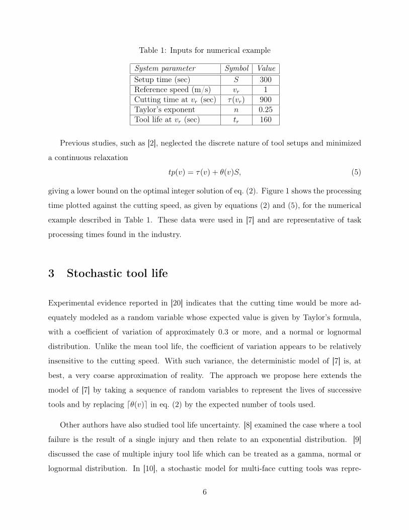
Table 1: Inputs for numerical example

System parameter Symbol ValueSetup time (sec) S 300Reference speed (m/s) vr 1Cutting time at vr (sec) τ(vr) 900Taylor’s exponent n 0.25Tool life at vr (sec) tr 160

Previous studies, such as [2], neglected the discrete nature of tool setups and minimized

a continuous relaxation

tp(v) = τ(v) + θ(v)S, (5)

giving a lower bound on the optimal integer solution of eq. (2). Figure 1 shows the processing

time plotted against the cutting speed, as given by equations (2) and (5), for the numerical

example described in Table 1. These data were used in [7] and are representative of task

processing times found in the industry.

3 Stochastic tool life

Experimental evidence reported in [20] indicates that the cutting time would be more ad-

equately modeled as a random variable whose expected value is given by Taylor’s formula,

with a coefficient of variation of approximately 0.3 or more, and a normal or lognormal

distribution. Unlike the mean tool life, the coefficient of variation appears to be relatively

insensitive to the cutting speed. With such variance, the deterministic model of [7] is, at

best, a very coarse approximation of reality. The approach we propose here extends the

model of [7] by taking a sequence of random variables to represent the lives of successive

tools and by replacing dθ(v)e in eq. (2) by the expected number of tools used.

Other authors have also studied tool life uncertainty. [8] examined the case where a tool

failure is the result of a single injury and then relate to an exponential distribution. [9]

discussed the case of multiple injury tool life which can be treated as a gamma, normal or

lognormal distribution. In [10], a stochastic model for multi-face cutting tools was repre-

6

0.4 0.45 0.5 0.55 0.6 0.65 0.7 0.75 0.8 0.85 0.91800

1900

2000

2100

2200

2300

2400

2500

Cutting velocity

Pro

cess

ing

time

__ deterministic tool life

−− continuous relaxation

.... exponential distribution

Figure 1: Processing time versus cutting speed

sented with the use of a normal or lognormal distribution when thermal or mechanical tool

fatigue occurs. An extension was proposed in [21] when tools are used to cut different parts,

based on conditional probabilities. Recently, [4] discussed a stochastic tool life model with

regard to tool inventory management.

In the present paper, we suppose the lives of the successive cutting tools are i.i.d. (in-

dependent and identically distributed) random variables Xi, i = 1, 2, . . ., with a given dis-

tribution. Let N(v) be the discrete random variable giving the number of tools required to

finish a part type at constant cutting speed v. We present a simple model to evaluate the

expected value N(v) = E[N(v)] of the number of tools used to process a single part type.

Decisions based on expected values are often justified in common manufacturing environ-

ments, because of the repetitive aspect of processing successive tasks. Equation (2) can then

be replaced by

TP (v) = τ(v) +N(v)S. (6)

Unlike equation (2), here we do not need to round up to the nearest integer since we are

7

calculating the expected value of a discrete, integer valued random variable. The expected

value itself does not have to be integer.

Let µ = E[Xi] be the mean tool life and σ2 = Var[Xi] = E[(Xi − µ)2] its variance.

We suppose the mean tool life is related to the cutting speed by Taylor’s formula, i.e.,

µ = t` = tr(v/vr)−1/n. Moreover, we suppose the coefficient of variation ξ = σ/µ is given

and is independent of the cutting speed v. This information is sufficient for determining

a tool life distribution with two parameters. For example, when Xi ∼ Gamma(r, λ), then

µ = r/λ and σ2 = r/λ2, so we obtain the two parameters:

r = 1/ξ2 and λ =r(v/vr)

1/n

tr. (7)

For the gamma distribution, there are three special cases of particular interest:

• Deterministic. Xi = t`, ξ = 0, r →∞.

• Exponential. Xi ∼ Exp(λ), ξ = 1, r = 1.

• Carbide tool. From Wager and Barash [20], ξ ≈ 0.3, so r ≈ 11 typically.

The exponential distribution represents tools with a highly variable lifetime, for example

when failure results from single injury. The expected processing time is plotted in Figure 1.

It is consistently larger than for a deterministic tool life, however the difference is always

bounded above by one setup time S. This is shown in the next section, where a method for

computing N(v) is also given.

It is well known (see, e.g., [11, 12, 13] that the exponential and gamma (with r ≥ 1)

distributions have an increasing failure rate (IFR). Also, any distribution such that ln(1 −

F (x)) is concave in x > 0 is IFR. On the other hand, a distribution such that ln(1− F (x))

is convex has a decreasing failure rate (DFR). The above discussion about the tool wear

process (and the discussion in [7]) would suggest that IFR distributions should be used to

model the tool life. Another reason for not using DFR distributions is that our convention

of a fixed coefficient of variation ξ may not be appropriate in this case.

8

In fact, as pointed out in [11], a common class of DFR distributions consists of mixtures of

exponential distributions. For example, one could imagine a certain tool has a probability p

of being of type 1, with Taylor parameters n1 = 0.18 and tr1 = 162.5, and a probability

1− p of being of type 2, with n2 = 0.28 and tr2 = 168.2. (In both cases, assume a reference

speed vr = 1.) This could be the case if the tool has been taken at random from one of two

toolboxes. For a tool of type i, i = 1, 2, Taylor’s relation will assign the parameter values

λi =1

tri

(v

vr

)1/ni

to the corresponding exponential distributions. Then each exponential distribution has a

coefficient of variation equal to 1, independent of the cutting speed, but the coefficient of

variation of the resulting hyperexponential distribution varies significantly with the cutting

speed, in contradiction with our convention and experimental evidence. For example, with

p = 0.7, we get ξ = 0.7609 at speed v = 0.7 and ξ = 0.6550 at speed v = 1.

4 Renewal process

We now find an expression for N(v). First, we denote τ = τ(v) as the cutting time used

to process a part. Let M(τ) be the random variable giving the number of tools needed for

processing during a certain time τ (so that the part is completed), i.e.,

M(τ)−1∑j=1

Xj < τ ≤M(τ)∑j=1

Xj.

Let M(τ) = E[M(τ)]. By construction N(v) = M(τ) so that N(v) = M(τ). Now {M(t)−

1, t ≥ 0} is a renewal process whose interarrival times are the random variables Xi, i =

1, 2, . . .. Then M(t) − 1 represents the corresponding renewal function. It is thus possible

to obtain this function from renewal theory, for example using Laplace transforms or a

numerical method. From the renewal function, we get N(v) = M(K1/v) by setting t = τ(v)

and using eq. (3).

There are two special cases for which the renewal function is trivial and thus M(t) is

easily obtained.

9

• Deterministic tool life: then Xj = t` with certainty and is given by equation (1).

So we get M(t) = 1 + bt/t`c. With t = τ(v), we derive N(v) = 1 + bK2vαc. Then eq.

(6) reduces to eq. (2), except at cutting speeds for which an integral number of tools

are used. (By convention, the renewal function counts all tool changes up to time t

inclusively, while in [7] the last tool setup was not counted if that tool was not used.)

• Exponential tool life: then Xj ∼ Exp(λ), which gives

M(t) = 1 + λt, for t ≥ 0. (8)

Replacing λ and t, we get

N(v) = 1 +K2vα. (9)

We remark that (6, 9) give exactly one extra setup time S when compared to (4, 5). This

explains the observation, in Figure 1, that when the tool life has an exponential distribution,

the expected processing time exceeds the lower bound of the continuous relaxation by exactly

one setup time.

Now let F (t) be the cumulative distribution function of the tool life, i.e., F (t) = P (Xi ≤

t). Let also the random variable Sk be the time at which the life of the kth tool ends, i.e.,

Sk = X1 + . . . + Xk, for k = 1, 2, . . .. By convention, let S0 = 0. For k = 0, 1, 2, . . ., define

the cumulative distribution functions Fk(t) = P (Sk ≤ t). Then F0(t) ≡ 1, F1(t) = F (t) and

Fk(t) is the k-fold convolution of F (t) with itself. Then from [11, Prop. 3.2.1], we have

M(t) =∞∑

k=0

Fk(t). (10)

If the tool life follows a gamma distribution with shape parameter r and scale parameter λ,

then Sk also has a gamma distribution but with shape parameter kr and scale parameter λ.

Then the functions Fk(t) can be computed using the incomplete gamma function, which is

available in standard scientific subroutine libraries. In this case, M(t) can be computed by

truncating the infinite sum in eq. (10). Similarly, if the tool life follows a discrete distribution

with a finite number of mass points, then the functions Fk(t) can be obtained using a standard

subroutine for discrete convolutions.

10

Another expression for M(t) can be obtained using Laplace transform analysis. We now

suppose the tool life Xi has an arbitrary continuous distribution with a Laplace transform.

Lemma 1 Let f(x) be the density function of Xi, and Lf (s) its Laplace transform. Then,

the Laplace transform of M(t) is given by

LM(s) =1/s

1− Lf (s). (11)

Proof. Let M̂(t) = M(t)− 1 be the renewal function of Xi, i = 1, 2, . . ., and m̂(t) = M̂ ′(t)

its renewal density. Then, their Laplace transforms are given by:

Lm̂(s) =Lf (s)

1− Lf (s)

LM̂(s) =Lf (s)/s

1− Lf (s).

Knowing that M(t) = M̂(t) + 1, ∀t ≥ 0, we obtain LM(s) = LM̂(s) + 1/s and the result

follows. 2

In some cases, it is possible to invert equation (11) using an expansion in partial frac-

tions. We now obtain the function M(t) in closed form when the tool life follows an Erlang

distribution (the gamma distribution with integer shape parameter r is called an Erlang

distribution). Recall the Laplace transform of an Erlang density is

Lf (s) =

s+ λ

)r

. (12)

The proofs of the following lemma and theorem are given in the appendix.

Lemma 2 Suppose Xi ∼ Erlang(r, λ), and let φk = ei2πk/r (the r-th unit root) and γk =

2(1− cos(2πk/r)) for k = 1, . . . , r − 1. Then

LM(s) =r + 1

2rs+

λ

rs2+

r−1∑k=1

(1− φk)/(rγk)

s+ (1− φk)λ. (13)

11

Theorem 3 Suppose Xi ∼ Erlang(r, λ) and let Ck = cos(2πk/r) and Sk = sin(2πk/r).

Then

M(t) =r + 1

2r+λt

r+

[1− (r mod 2)]

2re−2λt

+1

r

b(r−1)/2c∑k=1

e−(1−Ck)λt

{cos(Skλt) +

Sk sin(Skλt)

1− Ck

}. (14)

The function N(v) is obtained from (14) by taking r = 1/ξ2 (rounded to the nearest

integer) and substituting t = K1/v and λ = r(v/vr)1/n/tr as in (7). We can see that if r = 1

(exponential case) then equation (14) becomes M(t) = 1 + λt, as in (8). When r → ∞,

numerical computations show that TP (v) tends to the deterministic case. For example,

compare figures 1 and 2 (r = 10000).

0.4 0.45 0.5 0.55 0.6 0.65 0.7 0.75 0.8 0.85 0.91800

1900

2000

2100

2200

2300

2400

2500

Cutting velocity

Pro

cess

ing

time

__ r=10000

−. r=50

.... r=11

−− r=6

−. r=1

Figure 2: Processing time for gamma distribution

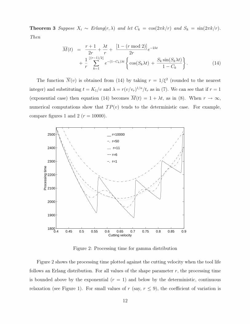
Figure 2 shows the processing time plotted against the cutting velocity when the tool life

follows an Erlang distribution. For all values of the shape parameter r, the processing time

is bounded above by the exponential (r = 1) and below by the deterministic, continuous

relaxation (see Figure 1). For small values of r (say, r ≤ 9), the coefficient of variation is

12

large (ξ ≥ 1/3), and the curves are in the upper half of the graph, with almost no oscillations.

On the other hand, for larger r there is less variability in the tool life and oscillations appear,

of greatest amplitude in the deterministic case, when r →∞.

5 Machine with tool magazine

In many manufacturing environments, machines are often equipped with a tool magazine.

This permits having a number of different tools immediately available for processing. We

suppose the setup times are negligible for tools that are preloaded into the magazine. More-

over, extra tools are manually inserted one by one in the machine when needed, and thus

each incurs a setup time S. Let TC be the number of tool slots in the magazine. The special

case TC = 0 corresponds to a machine with no tool magazine, as in the previous sections,

and for which all tools require a setup time.

Now let NTC(v) be the random variable of the number of tool setups needed to complete a

part at cutting speed v. With τ = τ(v) = K1/v the cutting time, we have NTC(v) = MTC(τ)

where the random variable MTC(τ) gives the number of tool setups that occur during a time

interval of duration τ . We now argue that {MTC(t), t ≥ 0} is a delayed renewal process. Let

Sk be the epoch of the kth tool loading. Then

S1 =TC∑j=1

Xj

is the instant when the last preloaded tool must be replaced. For k = 2, 3, . . ., we have

Sk = S1 +k−1∑j=1

XTC+j.

The interarrival times between successive tool loadings are therefore the i.i.d. random vari-

ables XTC+1, XTC+2, . . .. The time S1 of the first tool loading has a different distribution,

however, and the renewal process is thus delayed because of the tool magazine. From [11,

eq. (3.5.1)], the renewal function MTC(t) = E[MTC(t)] is given by

MTC(t) =∞∑

k=TC

Fk(t) = M(t)−TC−1∑k=0

Fk(t). (15)

Particular expressions are straightforward for three special cases.

13

• Deterministic tool life. As before, Xj = t` with certainty. So we get

MTC(t) = 1 +

⌊(t

t`− TC

)+⌋.

• Exponential tool life. Then Xj ∼ Exp(λ) and S1 ∼ Erlang(TC, λ). Let G0(t) ≡ 1

for t ≥ 0 and, for j = 1, 2, . . ., let Gj(t) be the cumulative distribution function of a

Erlang(j, λ). Then

MTC(t) = 1 + λt−TC−1∑k=0

Gk(t).

• Erlang tool life. If Xi ∼ Erlang(r, λ) then

MTC(t) = M(t)−TC−1∑`=0

Gr`(t), (16)

with M(t) given by eq. (14).

0.4 0.5 0.6 0.7 0.8 0.9 10

1

2

3

4

5

6

7

Cutting velocity

Too

l set

ups

__ exponential distribution

.... gamma distribution (r=50)

−− deterministic tool life

Figure 3: Tool setups versus cutting speed

The expected number of tool setups NTC(v) is obtained by substituting the correct values

for r, λ and t in (14, 16). Figure 3 shows N(v) and NTC(v) plotted against the cutting

14

speed, for a tool magazine of capacity TC = 2, compared to TC = 0. For the exponential

distribution, the expected number of tool setups when a tool magazine is present is near zero

at small speed but it remains positive. On the other hand, for tool life distributions with

small variance, the expected number of tool setups is much nearer zero in a significant range

of the cutting speed.

6 Minimizing the expected processing time

We now look at the problem of finding the cutting speed giving the minimum expected

processing time. For a flexible machine without a tool magazine, we simply minimize TP (v)

given by eq. (6). For a flexible machine with a tool magazine of capacity TC, we minimize

TP (v, TC) = τ(v) +NTC(v). (17)

Clearly, the special case with TC = 0 corresponds to a machine without a tool magazine

since TP (v, 0) = TP (v).

From this point on, we find it convenient to make a change of variable. Rather than

using the cutting speed v, we will use θ = θ(v), the corresponding quantity of tool used for

cutting the part type at speed v under Taylor’s deterministic tool life model, as given by eq.

(4). The cutting speed can easily be recovered from

v = (θ/K2)1/α.

Redefining the cutting time as ϕ(θ) = τ(v)/S, where S is the tool setup time, we get

ϕ(θ) = K3θ−1/α, (18)

with K3 = τ(vr)θ1/αr and θr = (τ(vr)/tr)

1/α is the amount of tool used at Taylor’s reference

cutting speed. We remark that the function ϕ(θ) is decreasing and convex provided α > 0.

This is true whenever the Taylor exponent n satisfies 0 < n < 1. Hence our analysis

is applicable to a wider range than was claimed in [7, Table 2], where only the interval

0 < n < 1/2 was considered.

15

We further remark that by setting t = τ(v) as in §4, then eq. (4) gives θ = t/t`. This

means θ expresses time in units of the mean tool life. Hence in the renewal process {M(t)−

1, t ≥ 0}, we can replace t by θ provided we choose the scale parameter of the interarrival

time distribution so that the expected tool life E[Xi] = 1. For the exponential distribution,

we would then have λ = 1, while for an Erlang distribution with shape parameter r, we

would have λ = r.

Under this convention, we then define the function

ωk(θ) = Nk(v) = Mk(θ) (19)

giving the expected number of tool setups under the cutting speed v, for a flexible machine

with a tool magazine of capacity TC = k tools. By construction, ωk(θ) gives the expected

number of renewals in excess of k−1 at time θ of a renewal process with unit mean interarrival

time. It increases with θ and it decreases with k. Moreover, it is easily shown that

ωk+1(θ)− ωk(θ) ≥ ωk(θ)− ωk−1(θ)

for any fixed value of θ, and for general tool life distribution. Hence the expected number

of tool setups is a discretely convex function of the magazine capacity. On the other hand,

for fixed k, the function ωk(θ) is not convex in θ, in general. There is one notable exception,

however.

Lemma 4 The function ωk(θ) is convex in θ for any given k when the tool life follows an

exponential distribution.

Proof.

ω′′k(θ) =∞∑

`=k

G′′` (θ) =

∞∑`=k

[g`−1(θ)− g`(θ)] = gk−1(θ) ≥ 0,

where g`(θ) = θ`−1/(`− 1)! is the `th Erlang density. 2

Nonetheless, even under exponential tool life, the function ωk(θ) is not jointly convex in k

and θ. For example, it is easily verified that

ω2(2) = 1.1353 > 1.1245 = 0.5[ω1(1) + ω3(3)].

16

Finally, for k = 0, 1, 2, . . ., we define the functions

ψk(θ) = ϕ(θ) + ωk(θ). (20)

Then the problem of minimizing eq. (20) is equivalent to minimizing eq. (17) with TC = k.

In particular, the optimal solutions θ∗k and v∗k satisty eq. (4) and the optimal values satisfy

TP (v∗k, k) = Sψk(θ∗k). Now let ψ∗k = ψk(θ

∗k), for k = 0, 1, 2, . . ..

Lemma 5 For general tool life distribution, the optimal solutions θ∗k are increasing and the

optimal values are decreasing: for k = 0, 1, 2, . . ., θ∗k+1 ≥ θ∗k and ψ∗k+1 ≤ ψ∗k.

Proof. This follows trivially from the fact that ψk(θ) = Fk(θ) + ψk+1(θ), where Fk(θ), the

probability distribution function of Sk = X1 + . . .+Xk, is increasing in θ. 2

The above argument also shows that ψ∗1 − ψ∗0 = −1 and θ∗0 = θ∗1. Also, in the special case of

the exponential distribution, the first-order optimality conditions give

θ∗0 = θ∗1 = ϕ−1(1) =(nK3

1− n

)1−n

.

Moreover, our numerical experience with the exponential and Erlang distributions of the

tool life suggest that these sequences have much stronger monotonicity properties, in fact.

Conjecture 6 Both the optimal solutions and the optimal values have increasing incre-

ments, with the increments of the optimal solutions being bounded above by 1: for k = 1, 2, . . .,

0 ≤ θ∗k − θ∗k−1 ≤ θ∗k+1 − θ∗k ≤ 1

−1 ≤ ψ∗k − ψ∗k−1 ≤ ψ∗k+1 − ψ∗k ≤ 0.

These monotonicity properties, when present, have two important consequences for com-

putations. One important consequence is that the discrete convexity of the optimal values ψ∗kallows the use of the greedy algorithm of [3] for allocating magazine capacity among multiple

part types as in [7]. Another consequence is to restrict the range for searching the optimal

solution for k+1 when θ∗k is given. Lower and upper bounds on the expected number of tool

17

setups can also be used to restrict the range of search for optimal solutions. For this, we

recall that a nonnegative random variable X is said to be new better than used in expectation

(NBUE) if

E[X − a | X > a] ≤ E[X] for all a ≥ 0.

It is well known that IFR distributions are also NBUE [11, 12, 13].

Lemma 7 For k = 0, 1, 2, . . ., and θ ≥ 0:

(θ − k)+ ≤ ωk(θ) ≤ 1 + θ −k−1∑`=0

G`(θ). (21)

where the lower bound is valid for general tool life distributions and the upper bound is valid

whenever the tool life distribution is NBUE.

Proof. The result is well known in the special case k = 0 (see, e.g., [11, 12, 13]): for a renewal

process with mean interarrival time 1/λ, the renewal function m(θ) is always bounded below

by λθ − 1, and if the distribution of the interarrival times is NBUE, it is bounded above by

λθ. (Here, by convention, we have λ = 1.) When k > 0, the lower bound follows from the

rightmost part of eq. (15) because M(θ) ≥ θ and F`(θ) ≤ 1. The upper bound, on the other

hand, follows from the middle part of eq. (15) by applying [11, Lemma 8.6.5]:

Mk(θ) =∞∑

`=k

F`(θ) ≤∞∑

`=k

G`(θ).

The result follows from the fact that

∞∑`=0

G`(θ) = 1 + θ.

2

Now suppose the tool life follows a NBUE distribution F (θ) and we want to find the

optimal solution θ∗k minimizing ψk(θ). Then Lemma 7 implies that

ϕ(θ) + (θ − k)+ ≤ ψk(θ) ≤ ψ̂k(θ),

where ψ̂k(θ) is the expected processing time when the tool life follows an exponential distri-

bution. But then both the lower and upper bounds are convex functions of θ. Now suppose

18

ψ̂∗k is the minimal value of ψ̂k(θ), then θk ≤ θ∗k ≤ θk where θk and θk are the two roots of the

equation

ϕ(θ) + (θ − k)+ − ψ̂∗k = 0.
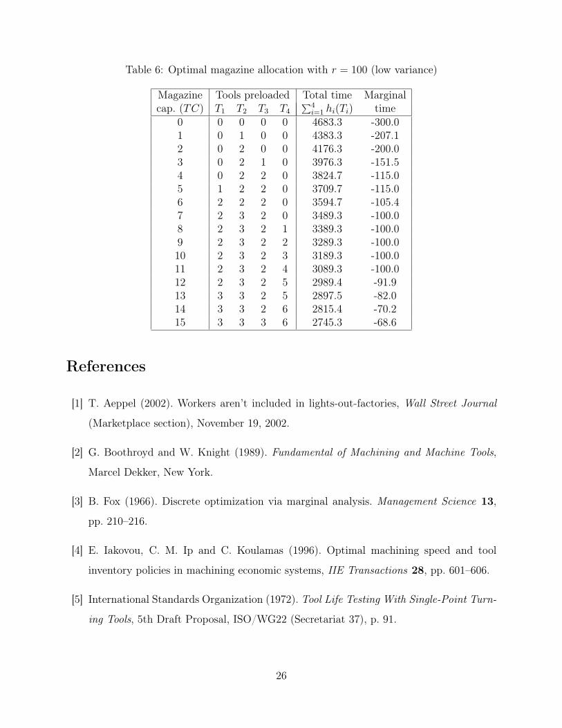
7 Numerical example

We now illustrate our stochastic tool life model with a numerical example, taken from [7], in

which the magazine capacity of TC = 15 tools has to be allocated optimally between four

different part types, and whose tool characteristics are given in Table 2. For a given part

type, and for TC = 0, 1, 2, . . ., we define the function

h(TC) = minv≥0

TP (v, TC)

where TP (v, TC) is the expected processing time given by eq. (17). Then h(TC) = Sψ∗TC .

Now as in [7], the problem of allocating the magazine capacity among the different part

types can be formulated as follows:

Min∑

i hi(Ti)s.t.

∑i Ti ≤ TC

Ti ≥ 0, integer

Table 2: Inputs for numerical example with four part types

Tool Part typescharacteristics 1 2 3 4S (seconds) 115 300 200 100vr (m/s) 1 1 1 1τ(vr) (seconds) 500 900 400 550n 0.25 0.18 0.28 0.38vrt

nr 3.2 2.5 4.2 5.0

Under the assumption of deterministic tool lives related to cutting speed by Taylor’s

equation, it was shown in [7] that the functions hi(Ti) have nondecreasing marginals, i.e.,

∆hi(Ti + 1) ≥ ∆hi(Ti), with ∆hi(Ti) = hi(Ti + 1) − h(Ti). The magazine capacity, in

this case, can then be allocated using the greedy method of [3], which increments Ti by

19

one whenever ∆hi(Ti) is the smallest marginal among all tool parts. Our computational

experience with stochastic tool life under exponential and Erlang distributions has been that

the same property seems to hold as well.

To investigate the effect of random tool life, we have computed the optimal tool allocation

for three different cases.

1. Worst case: exponential distribution (Erlang with r = 1) which has a coefficient of

variation ξ = 1.

2. Carbide tool: Erlang distribution with r = 11, with ξ ≈ 0.3.

3. Low variance: Erlang distribution with r = 100, with ξ = 0.1.

The detailed allocation results are given in the appendix (tables 4–6) and in [7, Table 8].

These results are summarized in Table 3 where

TP (v∗, TC) = expected processing time at deterministic optimal speed

TP ∗(TC) = optimal expected processing time,

and the numbers in parentheses give the increase in processing time relative to the deter-

ministic optimal value.

Table 3: Effect of random tool lives on optimal processing time

TC = 0 TC = 15Coef. var. TP (v∗) TP ∗ TP (v∗, TC) TP ∗(TC)

0 4500.1 4500.1 2632.1 2632.10.10 4865.9 4683.2 2994.9 2745.3

(8.1%) (4.1%) (13.8%) (4.3%)0.30 4888.1 4865.4 3042.6 2890.7

(8.6%) (8.1%) (15.6%) (9.8%)1 5215.1 5212.6 3559.0 3311.5

(15.9%) (15.8%) (35.2%) (25.8%)

These results show that the deterministic optimal processing times significantly under-

estimate the expected processing times by up to 16% for the exponential distribution (the

20

worst case) in the absence of a tool magazine, and up to 35% with a tool magazine of capac-

ity TC = 15. For a carbide tool, the underestimation is of nearly 9% and 16%, respectively.

Interestingly, the underestimation is only slightly smaller in the low variance case, with 8%

and 14%, respectively. These results thus make a strong case in favor of using a stochastic

model rather than a deterministic model for estimating the processing time when the tool

life is random and the tool setup times are not negligible. Further, Table 3 also shows that

the expected processing times can be reduced significantly by finding the optimal speed with

a stochastic model rather than using the deterministic optimal speed.

8 Conclusion

Using existing empirical relations of Taylor [18] and Wager and Barash [20] to express the

random tool life of a metal cutting tool as a function of cutting speed, we have developed

a model based on renewal theory to obtain the expected processing time of a metal cutting

task on a flexible machine tool. This model assumes that the tool life is a function of

cutting speed, and takes the cutting time as well as the tool setup time into account. A

correction term for machines equipped with a tool magazine has also been developed. We

presented a computational procedure valid when the tool life distribution is exponential

or gamma. Our method is illustrated with a numerical example showing the significant

impact of random tool life on the expected processing time. The model developed above

can be used to evaluate the consequences of machine-tool magazine configuration when

planning for lights-out/unmanned operations. The model supports the current focus in

manufacturing environments on single piece flow, rapid manufacturing response to demand

changes and waste reduction, increasing the competitiveness of manufacturers seeking to

exploit the opportunities that advances in tool-condition monitoring and on-line control now

offer.

21

9 Acknowledgements

This research was supported in part by the National Science and Engineering Research

Council of Canada, under Grant 0105560, and the Fonds pour la Formation de Chercheurs

et l’Aide à la Recherche du Québec, under grant 1570. The authors are also thankful to

the National Science Foundation for supporting this research through grant DMII: 9813177.

Martin Noël’s help with some of the computations is also acknowledged.

Appendix

Proof of Lemma 2

Substituting (12) in (11), we get

LM(s) =(s+ λ)r/s

(s+ λ)r − λr=

1

s+

λr

p(s), (22)

where

p(s) = s[(s+ λ)r − λr] = s2r−1∏k=1

(s+ (1− φk)λ).

Indeed, (φk − 1)λ is a root of p(s) because

[(φk − 1)λ+ λ]r − λr = φrkλ

r − λr = 0.

Writing LM(s) in partial fractions, we get

LM(s) =1

s+A0

s+B

s2+

r−1∑k=1

Ak

s+ (1− φk)λ. (23)

Equating (22) and (23), we get

λr = A0p(s)

s+B

p(s)

s2+

r−1∑k=1

Akp(s)

s+ (1− φk)λ. (24)

To find B, evaluate (24) at s = 0, applying L’Hospital’s rule twice:

λr = B lims→0

p(s)

s2= B

p′′(0)

2.

22

This gives

B =λ

r. (25)

Next, for ` = 1, . . . , r− 1, find A` by evaluating (24) at s = (φ` − 1)λ, applying L’Hospital’s

rule once:

λr = A` lims→(φ`−1)λ

{p(s)

s+ (1− φ`)λ

}= A` p

′((φ` − 1)λ).

Straightforward algebra then gives

A` =1− φ`

rγ`

. (26)

Finally, identify all terms in sr, giving

A0 = −r−1∑k=1

Ak.

If φk and φk′ are complex conjugate, then Ak+Ak′ = 1/r. Otherwise φk = −1 and Ak = 1/2r.

Hence

A0 = −r − 1

2r. (27)

Substitution of (25–27) in (23) yields (13). 2

Proof of Theorem 3

Direct inversion of Laplace transforms gives the first two terms of (14) from the first two

terms of (13). Direct inversion of the third term gives

r−1∑k=1

(1− φk

rγk

)e−(1−φk)λt.

The third term of (14) vanishes except for even r, in which case it corresponds to k = r/2,

so that φk = −1 and γk = 4.

The other terms can be grouped in complex conjugate pairs. Suppose φk and φk′ are a

conjugate pair, then (1− φk

rγk

)e−(1−φk)λt +

(1− φk′

rγk′

)e−(1−φk′ )λt

23

= 2<{(

1− φk

rγk

)e−(1−φk)λt

}

=2e−(1−Ck)λt

rγk

{[(1− Ck)− iSk]

× [cos(Skλt) + i sin(Skλt)]}

=2e−(1−Ck)λt

rγk

{(1− Ck) cos(Skλt)

+ Sk sin(Skλt)}.

Simplification yields the fourth term of (14). 2

Marginal allocation tables for stochastic tool life

We include here the detailed results of the numerical example for allocating a magazine

capacity of TC = 15 among four different part types, for three cases of stochastic tool life:

r = 1 (exponential), r = 11 (carbide tool) and r = 100 (low variance). The corresponding

table for deterministic tool life (r = ∞) is given in [7, Table 8].

24

Table 4: Optimal magazine allocation with r = 1 (exponential tool life)

Magazine Tools preloaded Total time Marginalcap. (TC) T1 T2 T3 T4

∑4i=1 hi(Ti) time

0 0 0 0 0 5212.5 -300.01 0 1 0 0 4912.5 -201.52 0 2 0 0 4711.0 -200.03 0 2 1 0 4511.0 -139.44 0 2 2 0 4371.6 -129.65 0 3 2 0 4242.0 -115.06 1 3 2 0 4127.0 -100.27 2 3 2 0 4026.9 -100.08 2 3 2 1 3926.9 -99.19 2 3 2 2 3827.8 -95.110 2 3 2 3 3732.7 -90.611 2 4 2 3 3642.2 -89.412 2 4 3 3 3552.8 -87.013 2 4 3 4 3465.8 -77.614 3 4 3 4 3388.1 -76.715 3 4 3 5 3311.5 -67.8

Table 5: Optimal magazine allocation with r = 11 (carbide tool)

Magazine Tools preloaded Total time Marginalcap. (TC) T1 T2 T3 T4

∑4i=1 hi(Ti) time

0 0 0 0 0 4865.4 -300.01 0 1 0 0 4565.4 -225.02 0 2 0 0 4340.4 -200.03 0 2 1 0 4140.4 -163.34 0 2 2 0 3977.0 -116.75 0 3 2 0 3860.3 -115.06 1 3 2 0 3745.3 -114.27 2 3 2 0 3631.1 -100.08 2 3 2 1 3531.1 -100.09 2 3 2 2 3431.1 -100.010 2 3 2 3 3331.1 -99.811 2 3 2 4 3231.3 -93.112 2 3 2 5 3138.2 -91.513 3 3 2 5 3046.7 -79.314 3 3 3 5 2967.3 -76.615 3 3 3 6 2890.7 -75.9

25

Table 6: Optimal magazine allocation with r = 100 (low variance)

Magazine Tools preloaded Total time Marginalcap. (TC) T1 T2 T3 T4

∑4i=1 hi(Ti) time

0 0 0 0 0 4683.3 -300.01 0 1 0 0 4383.3 -207.12 0 2 0 0 4176.3 -200.03 0 2 1 0 3976.3 -151.54 0 2 2 0 3824.7 -115.05 1 2 2 0 3709.7 -115.06 2 2 2 0 3594.7 -105.47 2 3 2 0 3489.3 -100.08 2 3 2 1 3389.3 -100.09 2 3 2 2 3289.3 -100.010 2 3 2 3 3189.3 -100.011 2 3 2 4 3089.3 -100.012 2 3 2 5 2989.4 -91.913 3 3 2 5 2897.5 -82.014 3 3 2 6 2815.4 -70.215 3 3 3 6 2745.3 -68.6

References

[1] T. Aeppel (2002). Workers aren’t included in lights-out-factories, Wall Street Journal

(Marketplace section), November 19, 2002.

[2] G. Boothroyd and W. Knight (1989). Fundamental of Machining and Machine Tools,

Marcel Dekker, New York.

[3] B. Fox (1966). Discrete optimization via marginal analysis. Management Science 13,

pp. 210–216.

[4] E. Iakovou, C. M. Ip and C. Koulamas (1996). Optimal machining speed and tool

inventory policies in machining economic systems, IIE Transactions 28, pp. 601–606.

[5] International Standards Organization (1972). Tool Life Testing With Single-Point Turn-

ing Tools, 5th Draft Proposal, ISO/WG22 (Secretariat 37), p. 91.

26

[6] S. Kurada and C. Bradley (1997). A review of machine vision sensors for tool condition

monitoring, Computers in Industry 34, pp. 55–72.

[7] B. F. Lamond and M. S. Sodhi (1997). Using tool life models to minimize processing

time on a flexible machine. IIE Transactions 29, pp. 611–621.

[8] S. Ramalingam and J. D. Watson (1977). Tool-life distributions, Part 1: Single-injury

tool-life model, J. Eng. Ind. 99, pp. 519–522.

[9] S. Ramalingam (1977). Tool-life distributions, Part 2: Multiple-injury tool-life model,

J. Eng. Ind. 99, pp. 523–530.

[10] S. Rosetto and A. Zompie (1981). ‘A stochastic tool-life model, Trans. ASME 103, pp.

126–129.

[11] S. M. Ross (1983). Stochastic Processes. Wiley, New York.

[12] M. Shaked and J. G. Shanthikumar (1994). Stochastic Orders and Their Applications,

Academic Press, San Diego.

[13] D. Stoyan (1983). Comparison Methods for Queues and Other Stochastic Models, Wiley,

New York.

[14] M. S. Sodhi, B. F. Lamond, A. Gautier and M. Noël (2001). Heuristics for determin-

ing economic processing rates in a flexible manufacturing system. European Journal of

Operational Research 129:1, pp. 105–115.

[15] J. Talavage and R. G. Hannam (1987). Flexible Manufacturing Systems in Practice:

Applications, Design and Simulation, Wiley, New York.

[16] C. S. Tang and E. V. Dernardo (1988). Models arising from flexible manufacturing

machine, Part 1: Minimization of the number of tool switches, Operations Research 36,

pp. 767–777.

[17] C. S. Tang and E. V. Dernardo (1988). Models arising from flexible manufacturing

machine, Part 2: Minimization of the number of switching instants", Operations Re-

search 36, pp. 778–784.

27

[18] F. W. Taylor (1906). “On the Art of Cutting Metals, Trans. ASME, 28, pp. 310–350.

[19] M.A. Trick, 1994, Scheduling multiple variable-speed machines, Operations Research 44,

pp. 234–248.

[20] A. B. Wager and M. Barash (1971). Study of the distribution of the life of HSS tools,

Trans. ASME 93, pp. 1044–1050.

[21] C. Zhou and R. A. Wysk (1992). Tool status recording and its use in probabilistic

optimization, J. Eng. Ind. 114, pp. 494–499.

28


Recommended