Document downloaded from:

http://hdl.handle.net/10459.1/59392

The final publication is available at:

https://doi.org/10.1007/s11069-015-1759-x

Copyright

(c) Springer, 2015

Natural Hazards

Climate change influence on runoff and soil losses in a rainfed basin withMediterranean climate

--Manuscript Draft--

Manuscript Number: NHAZ-D-14-00945R3

Full Title: Climate change influence on runoff and soil losses in a rainfed basin withMediterranean climate

Article Type: Manuscript

Keywords: climate change; evapotranspiration; runoff; soil losses; soil water; vines

Corresponding Author: Jose Martinez-Casasnovas, Ph.D.University of LleidaLleida, Not Applicable SPAIN

Corresponding Author SecondaryInformation:

Corresponding Author's Institution: University of Lleida

Corresponding Author's SecondaryInstitution:

First Author: M Concepción Ramos, Ph.D.

First Author Secondary Information:

Order of Authors: M Concepción Ramos, Ph.D.

Jose Martinez-Casasnovas, Ph.D.

Order of Authors Secondary Information:

Funding Information: Spanish Ministry of Science andInnovation(AGL2009-08353)

M Concepción RamosDr Jose Martinez-Casasnovas

Abstract: The present research shows the results of possible effects of climate change on runoffand soil loss in a rainfed basin located in the Alt Penedès and Anoia region (NE Spain).Viticulture is an important economic activity in this region and vines for production ofhigh quality wines and "cavas" are the main land use. Climate data for the period 2000-2012 and detailed soil and land use maps were used as input data for SWAT (Soil andWater Assessment Tool) to model the effects of climate change. The analysiscompared simulated results for years with different climatic conditions during thatperiod with predicted temperature and precipitation data for 2020, 2050 and 2080based on data obtained from the HadCM3A2 (Hadley Centre Coupled Model, version3, A2 scenario) and the trends observed in the area. The research confirmed thedifficulty of predicting future soil loss in this region, which has very high inter-annualclimate variability. Despite only small changes in precipitation, the model simulated adecrease in soil loss associated with a decrease in runoff, mainly driven by an increasein evapotranspiration. However, the trend in soil losses may vary when changes inprecipitation balance the increase in evapotranspiration and when rainfall intensityincreases. An increase in maximum rainfall intensity in spring and autumn (main rainyseasons) produced significant increases in soil loss: as high as 12% for the 2020scenario and 57% for the 2050 scenario.

Response to Reviewers: > Small comments by Reviewer #1:> L93: "vines occupied 62.9% of the basin" this value is different from the previouslycited 62.8% (L49). Please verify the correct value.

Answer: We have changed the value to 62.9% in the text.

> L154: Please add reference where reader can find the observed trends.

Answer: The reference has been added. It was already listed in the reference list.

Powered by Editorial Manager® and ProduXion Manager® from Aries Systems Corporation

> L228-229: "Camps and Ramos, 2010" is not listed in reference. Please, verify all thereferences cited in the text and the listed references.

Answer: It has been corrected. It was 2012 instead of 2010 and it also was listed in thereference list.

> L277: Is it correct the dot before "The increse in temperature..."?

Answer: The point has been changed to a comma.

Powered by Editorial Manager® and ProduXion Manager® from Aries Systems Corporation

2

Climate change influence on runoff and soil losses in a rainfed basin with

Mediterranean climate

M. C. Ramos (*) & J. A. Martínez-Casasnovas

Department of Environment and Soil Sciences. University of Lleida. Lleida, Spain.

*Corresponding author: Tel +34 973702092; Fax: +34 973702613; email:cramos@macs.udl.es

Abstract The present research shows the results of possible effects of climate change on runoff and

soil loss in a rainfed basin located in the Alt Penedès and Anoia region (NE Spain). Viticulture is an

important economic activity in this region and vines for production of high quality wines and “cavas”

are the main land use. Climate data for the period 2000-2012 and detailed soil and land use maps were

used as input data for SWAT (Soil and Water Assessment Tool) to model the effects of climate

change. The analysis compared simulated results for years with different climatic conditions during

that period with predicted temperature and precipitation data for 2020, 2050 and 2080 based on data

obtained from the HadCM3A2 (Hadley Centre Coupled Model, version 3, A2 scenario) and the trends

observed in the area. The research confirmed the difficulty of predicting future soil loss in this region,

which has very high inter-annual climate variability. Despite only small changes in precipitation, the

model simulated a decrease in soil loss associated with a decrease in runoff, mainly driven by an

increase in evapotranspiration. However, the trend in soil losses may vary when changes in

precipitation balance the increase in evapotranspiration and when rainfall intensity increases. An

increase in maximum rainfall intensity in spring and autumn (main rainy seasons) produced

significant increases in soil loss: as high as 12% for the 2020 scenario and 57% for the 2050 scenario.

Key words climate change; evapotranspiration; runoff; soil losses; soil water; vines.

ManuscriptClick here to view linked References

2

1 Introduction 1

Climate change adds an element of uncertainty to the magnitude of erosion processes. These processes, 2

frequently observed in the Mediterranean region, could be considerably affected by predicted changes in 3

rainfall characteristics. Different studies carried out in the Mediterranean region suggest that notable 4

changes in seasonal precipitation regimes occurred during the second half of the 20th

century. For 5

example, in Spain, González-Hidalgo et al. (2010) and Ramos et al. (2012) observed changes affecting 6

the main rainy seasons, with a negative trend in spring (between March and June in all Spanish basins) 7

and a positive one in October. In an analysis carried out for the period 1901-2008 in France, Hirschi and 8

Seneviratne (2010) observed a decreasing trend in spring-to-autumn correlations. However, precipitation 9

extremes seem to increase in association with global warming (Easterling et al., 2000; Klein Tank and 10

Können, 2003; Kharin et al., 2007), which may favour erosion processes (Favis-Mortlock and Boardman, 11

1995; Ramos and Martínez-Casasnovas, 2009). 12

Agriculture, and in particular perennial crops, may be extremely vulnerable to climate change. 13

Changes in temperature, associated with a more irregular distribution of rainfall which affects crop 14

production, tend to result in an increase in water demand. In addition, some typical Mediterranean land 15

uses with only limited soil cover, as in the cultivation of vines, olives, almonds and/or hazelnuts, are 16

usually associated with higher rates of erosion (Kosmas et al., 1997). In these cases, the increase in the 17

number of extreme precipitation events may have an additional impact, with greater water volumes being 18

lost to runoff and higher erosion rates. These increasing erosion rates imply not only a soil threat that 19

affects the sustainability of the ecosystem, but also significant economic losses for the agricultural sector. 20

The economic impact of soil erosion is difficult to quantify, although it is known that it also affects 21

nutrient losses and supposes additional labour costs in the fields. Estimations carried out in the study area 22

indicate that soil losses in vineyards represent about 9% of income from grape sales (Martínez-23

Casasnovas and Ramos, 2006). Other authors have estimated the cost of nutrient losses by erosion at 24

$2.10 per Mg of eroded soil and have also calculated additional costs related to off-site effects (Iowa 25

Learning Farms, 2013). In addition, large-scale estimations in Europe (Panagos and Montaranella, 2014) 26

indicate that the cost of soil loss ranges between 0.27 and 5.7 €/ha yr-1

, depending on the land cover. 27

Predictions of the impact of climate change on erosion rates have been made for several different 28

environments and according to different scenarios (Nearing et al., 2005; Dadson et al., 2010; Zhang et al., 29

3

2012). One of the various models used for these predictions is the Soil and Water Assessment Tool 30

(SWAT) which includes mechanisms to model the effects of climate change. SWAT has been applied by 31

several authors with this purpose in mind, though mainly in large basins (Nunes and Nearing, 2011; Bang 32

et al., 2013; Mukundan et al., 2013). 33

Given the importance of the sustainability of vine cultivation in Mediterranean areas, the 34

objective of the present study was to analyse the possible effects of climate change on runoff and soil 35

losses in a sample rainfed basin with a Mediterranean climate mainly cultivated with vines. The SWAT 36

model was used to simulate annual runoff and soil losses using daily data for the period 2000-2012 which 37

includes years of differing characteristics. Two years were selected as representative years of average 38

precipitation but with different rainfall distributions throughout the year, and a wetter year was 39

additionally selected which included some extreme rainfall events. The results obtained for these years 40

were compared with values simulated for three future scenarios (2020, 2050 and 2080) based on data 41

obtained from the HadCM3A2 (Hadley Centre Coupled Model, version 3, A2 scenario) and the climate 42

trends observed in the study area. 43

44

2 Material and methods 45

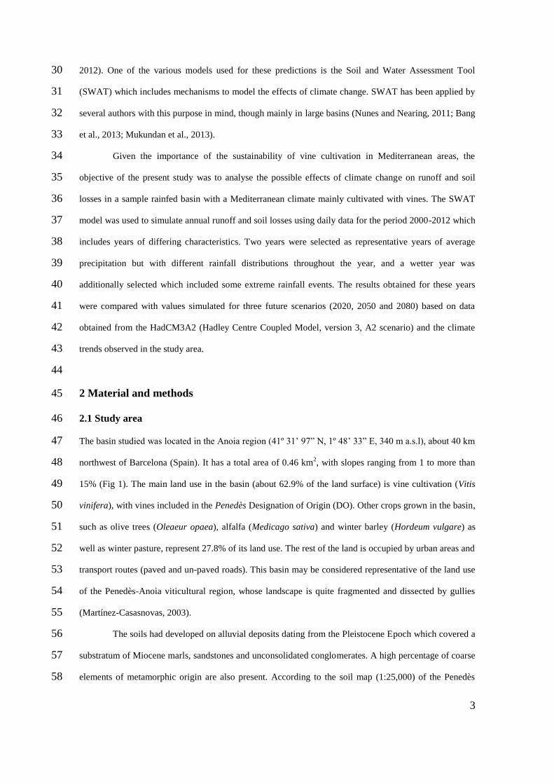
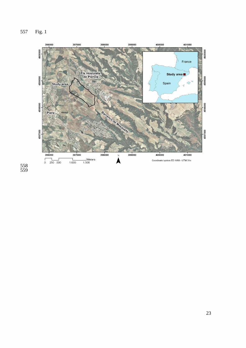
2.1 Study area 46

The basin studied was located in the Anoia region (41º 31’ 97” N, 1º 48’ 33” E, 340 m a.s.l), about 40 km 47

northwest of Barcelona (Spain). It has a total area of 0.46 km2, with slopes ranging from 1 to more than 48

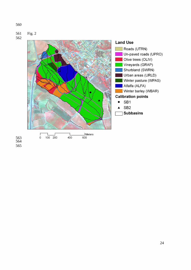
15% (Fig 1). The main land use in the basin (about 62.9% of the land surface) is vine cultivation (Vitis 49

vinifera), with vines included in the Penedès Designation of Origin (DO). Other crops grown in the basin, 50

such as olive trees (Oleaeur opaea), alfalfa (Medicago sativa) and winter barley (Hordeum vulgare) as 51

well as winter pasture, represent 27.8% of its land use. The rest of the land is occupied by urban areas and 52

transport routes (paved and un-paved roads). This basin may be considered representative of the land use 53

of the Penedès-Anoia viticultural region, whose landscape is quite fragmented and dissected by gullies 54

(Martínez-Casasnovas, 2003). 55

The soils had developed on alluvial deposits dating from the Pleistocene Epoch which covered a 56

substratum of Miocene marls, sandstones and unconsolidated conglomerates. A high percentage of coarse 57

elements of metamorphic origin are also present. According to the soil map (1:25,000) of the Penedès 58

4

region (DAR, 2008), the most frequent soils in the basin are classified as Typic Xerorthents and Fluventic 59

Haploxerepts. The basin drains into a gully system, which is characteristic of the landscape of the region 60

in which it is located (Martínez-Casasnovas and Ramos, 2009). 61

62

2.2 Runoff and soil loss simulation: Soil and Water Assessment Tool 63

The Soil and Water Assessment Tool (SWAT) (Nearing et al., 2005) was used to model the effects of 64

climate change on runoff and soil losses. SWAT simulates the hydrological water balance of the basin on 65

the basis of hydrological response units (HRU), which are obtained from a combination of soil, land use 66

and slope degree characteristics. The model operates on a daily time step. Flow and water quality 67

variables are routed from the HRU to subbasins and subsequently to the watershed outlet. SWAT 68

simulates hydrological processes as a two-component system comprised of surface hydrology and 69

channel hydrology, as described by Neitsch et al. (2011). It integrates various models: the Soil 70

Conservation Service curve number technique (USDA-SCS, 1985) is used to estimate runoff rates; the 71

modified soil loss equation, MUSLE (Williams and Berndt, 1977), is used for erosion and sediment yield 72

at basin scale; and the routing of channel sediment is simulated through a modification of Bagnold’s 73

sediment transport equation (Bagnold, 1977). Simulations in this work were carried out using ArcSWAT 74

2009.93.5, run at daily time steps. 75

76

2.2.1 SWAT input data 77

The required inputs for SWAT, referring to climate, soil and topographic characteristics, as well as 78

management practices and operations, are described below. 79

80

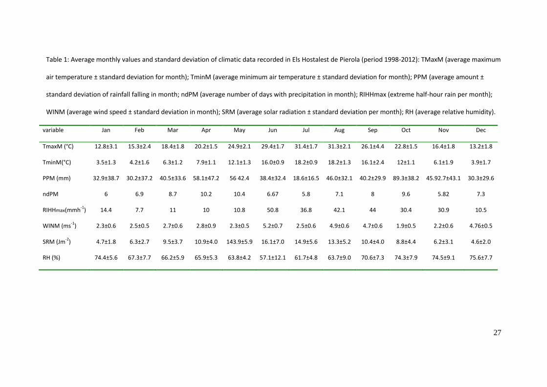
Climatic data 81

Climatic data were taken, on a daily basis, from the Els Hostalest de Pierola observatory (EHP: 41º 31’ 82

58” N, 1º37’45”E; 316 m a.s.l.), run by the Catalonian Meteorological Service (Servei Meteorològic de 83

Catalunya) and located 2.5 km from the basin. Both daily data and the average monthly values for a 15-84

year series (1998-2012) of maximum and minimum temperatures, precipitation, solar radiation, relative 85

humidity and wind speed were considered when running the model. The average values of these variables 86

are shown in Table 1. Precipitation was also recorded at 1-min intervals at the basin outlet, in order to 87

5

determine the rainfall intensity. This rainfall intensity was used, in combination with the steady 88

infiltration rate, to estimate the runoff rates. 89

90

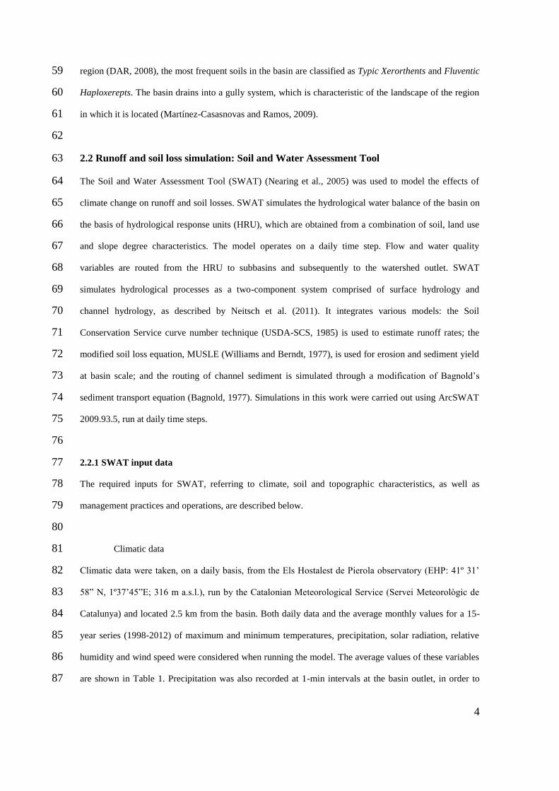
Land use and crop characteristics 91

The land uses in the basin were derived from orthorectified aerial photos taken in 2010 at a scale of 92

1:3,000 and from field work. This survey showed that vines occupied 62.9% of the basin. Other minor 93

crops present in the basin were: olive trees (4.79%), alfalfa (8.5%), winter barley (9.4%), winter pasture 94

(1.5%) and scrub (3.6%). Urban areas, including residential areas, paved and un-paved roads and tracks, 95

represented about 9.3% of the total surface area (Fig 2). Crop parameters were taken from the SWAT data 96

base and updated withinformation that had been obtained in previous works carried out in the study area 97

related to biomass, P and N concentrations. Crop fertilization (composition, doses and timetable) and 98

tillage operations (type and timetable) for each crop were supplied by the owners of the agricultural fields 99

in the basin. 100

101

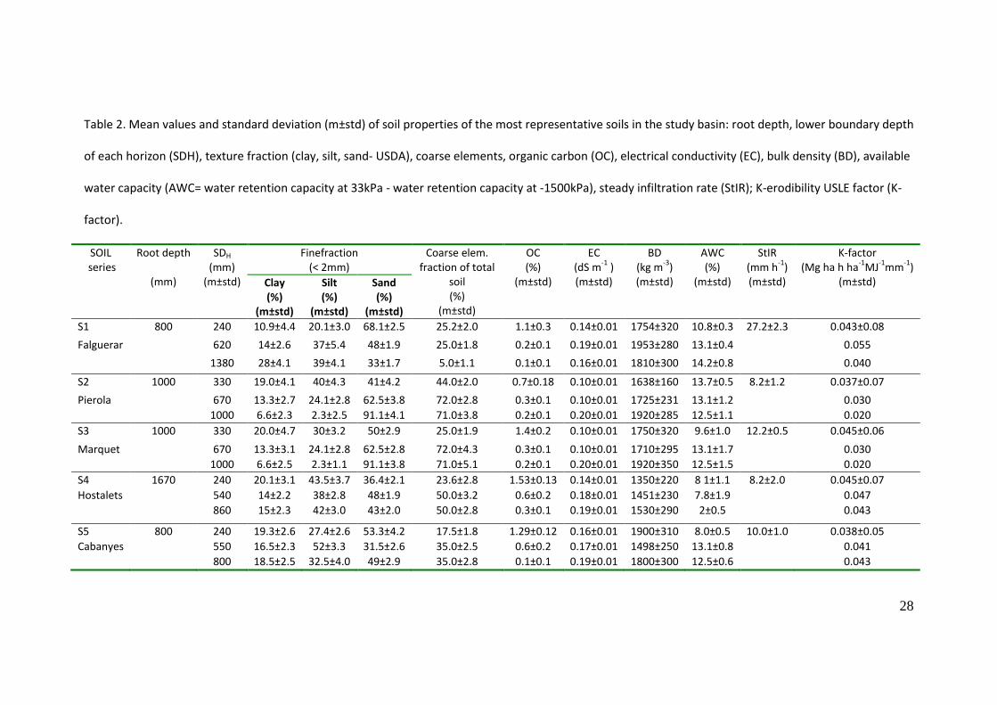
Soil and topographic characteristics 102

Soil characteristics were extracted from a soil map (1:25,000) (DAR, 2008). Additional top soil 103

properties, such as soil particle distribution, bulk density, organic carbon, water retention capacity (at 104

saturation, at -33 kPa and at -1500 kPa) and infiltration capacity, were obtained from our own soil survey 105

conducted with a density of 1 sample per ha. The locations of the samples were based on differences in 106

the multi-spectral responses of soils which were seen in a false colour composite of a WorldView-2 107

image acquired in July 2010. The soil erodibility factor (KUSLE factor) was also computed for each soil 108

unit using the equation proposed by Wischmeier and Smith (1971). 109

Table 2 shows the average characteristics of the main soil types found in the basin. Most of the 110

soils analysed have loamy or loamy-sandy textures, with a relatively high proportion of coarse elements 111

of metamorphic origin. The organic matter content of these soils is relatively low and some soils in the 112

basin are highly erodible (with relatively high KUSLE factor). The available water capacity and steady 113

infiltration rate of the soils presented high variability within the basin, contributing to the generation of 114

differences in soil water content and runoff rates. Soils are moderately deep, with maximum depths of 115

about 110 cm. None of the soils sampled presented redox depletions, indicating a good circulation of 116

drainage water within the soil profile. 117

6

A 1m-resolution digital elevation model of the study area, generated from a low-altitude 118

photogrammetric aerial survey carried out in 2010, was also used. SWAT HRUs were defined by 119

considering slope intervals of 0-2, 2-5, 5-10, 10-15 and >15%. The combination of soil type, slope and 120

land use data generated thirty-four subbasins and HRUs within the basin. The size of the different HRUs 121

ranged from 0.1 to 5.5 ha. 122

2.2.2. Model calibration and validation 123

Model calibration and validation were carried out in a previous work (Ramos and Martínez-Casasnovas, 124

2014) using data collected from two subbasins, SB1 and SB2, in which vines were cultivated (Fig. 2). In 125

that work, a sensitivity analysis was conducted to identify and rank the parameters that most affected the 126

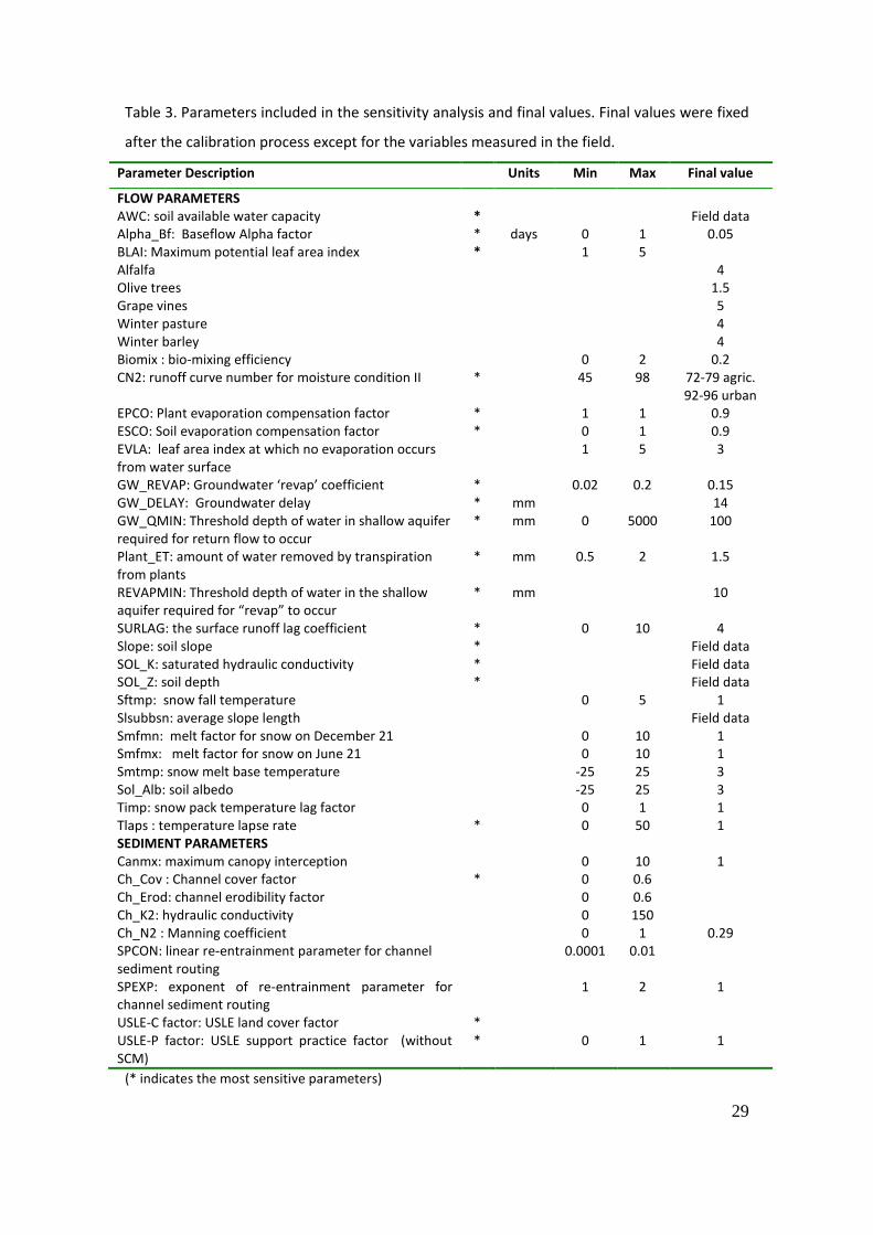
response of the model, and the rate of change of the outputs with respect to changes in the inputs. Table 3 127

lists the parameters used in the analysis and those that were the most sensitive. The most sensitive 128

parameters, excluding those measured in the field, were manually changed one at a time until the best fit 129

was obtained between measured and simulated values of soil water content, runoff and sediment yield in 130

the two analysed subbasins. Soil water was measured in the subbasins SB1 and SB2 using TFD Decagon 131

capacitance probes installed at different depths (10-30, 30-50, 50-70 and 70-90 cm). The probes were 132

calibrated by comparison with soil water contents measured by gravimetry. Runoff samples were 133

collected after the main rainfall events recorded during the calibration period using Gerlach troughs. 134

Runoff rates were calculated after each rainfall event by considering steady infiltration rates, estimated by 135

rainfall simulation in each subbasin (Ramos and Martínez-Casasnovas, 2010), and the antecedent soil 136

moisture. It was considered that rainfall whose intensity is greater than the steady infiltration rate is 137

unable to infiltrate and runs off, as well as water that falls when the soil is under saturation conditions. 138

The results obtained were then used in conjunction with runoff water volumes to calculate soil losses. 139

This was done for each runoff sampling point and the results were compared with simulated soil losses. 140

The obtained runoff and erosion rates were compared with simulated values in the two subbasins. 141

Model performance in the calibration and validation periods was defined on the basis of three 142

statistics: Nash-Sutcliffe efficiency (NSE; Nash and Sutcliffe, 1970); percent bias (PBIAS, %; Gupta et 143

al., 1999) and the ratio of the root mean square error to the standard deviation (RSR). According to the 144

criteria proposed by Moriasi et al. (2007), the statistics generated produced satisfactory results for both 145

calibration and validation periods. The results obtained are given in Ramos and Martínez-Casasnovas 146

(2014). 147

7

2.2.3 Climate change simulated scenarios 148

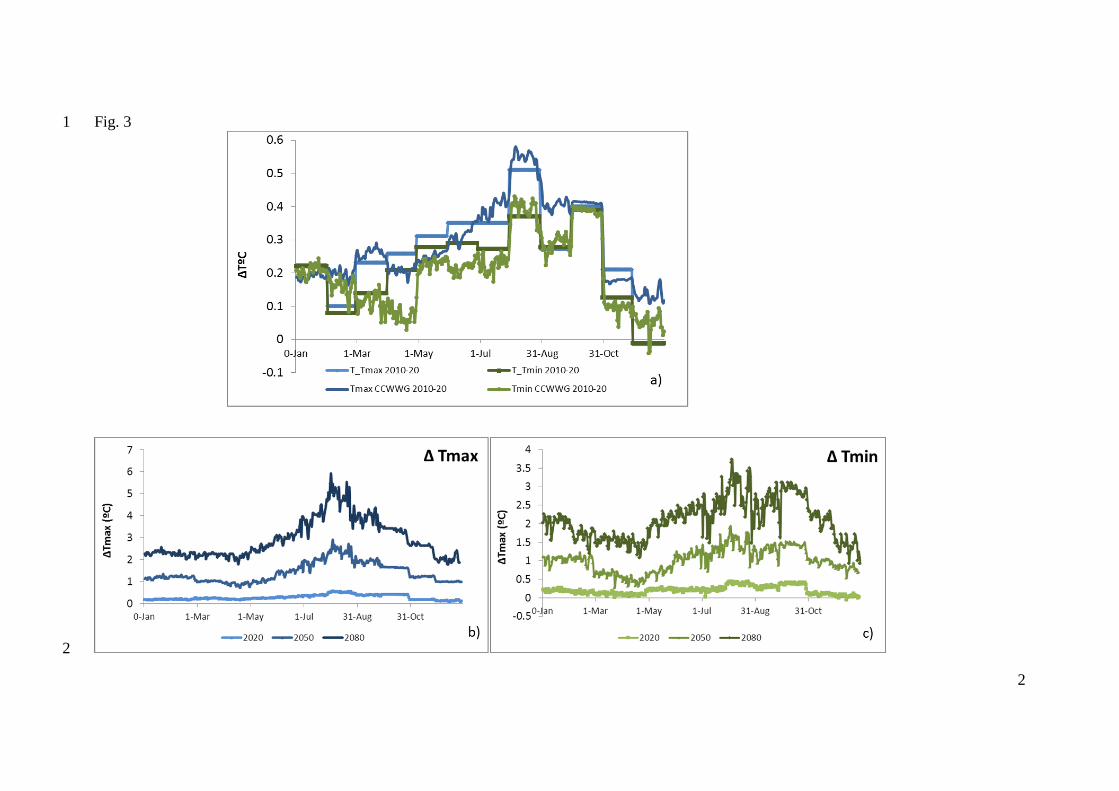
Three scenarios (2020, 2050 and 2080) were simulated taking into account estimated temperature, 149

precipitation, solar radiation and humidity. Changes in temperature, humidity and solar radiation were 150

simulated using the CCWorldWeatherGen climate change world weather file generator V1.6 (Jentsch et 151

al., 2012). This model uses data of the HadCM3 A2 (Hadley Centre Coupled Model, version 3 under the 152

A2 scenario). The generated temperature series were compared with the changes projected for the same 153

scenarios taking into account the trends observed in the area in the last years (Ramos et al., 2012). 154

Figure 3a shows the changes in Tmax and Tmin simulated for the 2020 scenario with the 155

CCWorldWeatherGen as well as the average monthly changes derived from the observed trends in the 156

area. It can be seen that there was good agreement on annual mean temperature, although the observed 157

trends represented higher values in spring and autumn and slightly lower values in summer. According to 158

the observed trends for the period 2010-2020, maximum temperature would increase by about 0.28 ºC, 159

while the increase for minimum temperature could be about 0.2 ºC, though with a greater increase in 160

spring (up to 0.4 ºC) and summer (up to 0.57 ºC). For the 2050 scenario, the projected annual temperature 161

changes would be +1.76 ºC for Tmax and 1.27 ºC for Tmin, and for the 2080 scenario, the projected 162

changes would be +3.3 ºC for Tmax and 2.4 ºC for Tmin, on average, with greater change ratios being 163

observed in spring and autumn than in winter. Figure 3b and 3c show the predicted changes in Tmax and 164

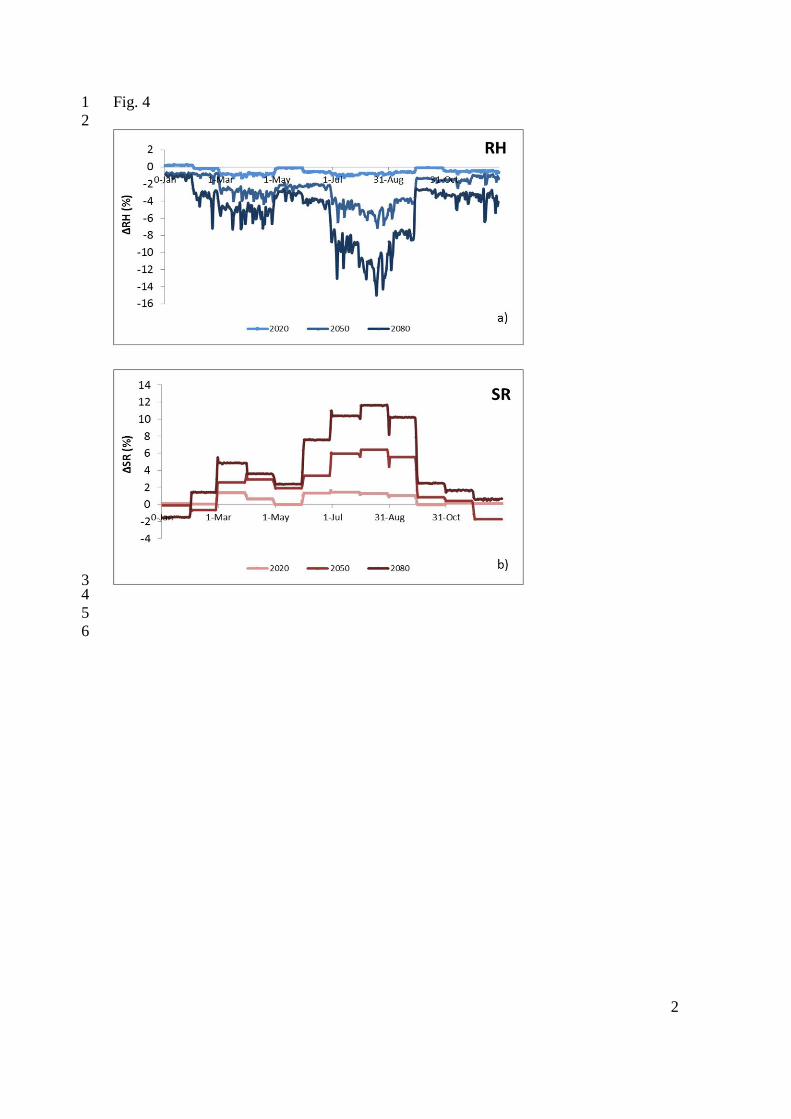
Tmin respectively for the scenarios 2020, 2050 and 2080, simulated with the CCWorldWeatherGen in 165

relation to the present day. Similarly, Fig. 4 shows the simulated changes for a) Relative Humidity (RH) 166

and b) Solar Radiation (SR) for the three scenarios. Changes in solar radiation ranged between 1 and 12% 167

and changes in relative humidity varied between less than 1% in the winter months and about -16% in 168

summer. 169

For precipitation, the high variability from year to year observed in the area made it difficult to 170

establish clear trends. The trends observed by Ramos et al. (2012) implied only small changes in rainfall. 171

Total precipitation did not change significantly, but a slight tendency for spring precipitation to decrease 172

(0.25% per year) and for late autumn-winter precipitation to increase (0.42% per year) was observed. 173

Downward trends were observed in summer and early autumn, although at a smaller rate (0.089 and 174

0.025% per year, respectively). These change ratios, representing respectively for the 2020, 2050 and 175

2080 scenarios increases of 4.2, 16.8 and 29.4% of rainfall in winter, and decreases of 2.5, 10 and 17.5% 176

in spring, 0.89, 3.6 and 6.3% in summer and 0.25, 1.2 and 2.1% in autumn, were considered in this 177

8

analysis. For the three selected years (2003, 2007 and 2011), with different rainfall distribution 178

throughout the years, the change ratios represented, respectively, increases in annual rainfall of 2.74, 3.5 179

and 1.1% for the 2020 scenario, 4.52, 5.03 and 3.98% for the 2050 scenario and 5.88, 7.28 and 6.25% for 180

the 2080 scenario. 181

The number of erosive events in the region has increased during the years 1997-2013(Ramos and 182

Durán, 2014). In addition, 30-min rainfall intensity, commonly used to estimate rainfall erosivity, also 183

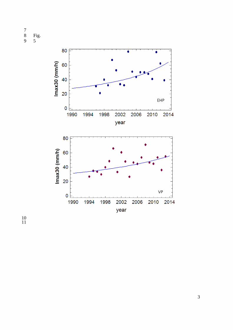
showed an upward trend over the same period (Fig. 5). The analysis carried out for the Els Hostalest de 184

Pierola observatory (EHP: 41º 31’ 97” N, 1º 48’ 33” E, 326 m a.s.l.) and for Vilafranca del Penedès 185

observatory (VP: 41º 19’ 59” N, 1º 40’ 40” E, 202 m a.s.l.), showed that 30-min rainfall intensity was 186

between 12 and 25% greater during the last 10 years (2004-2013) than in previous years. The EHP 187

observatory, the higher of the two observatories, recorded greater changes in rainfall intensity as well as 188

the highest values (up to 78.8 mmh-1

in EHP and about 70 mmh-1

in VP). 189

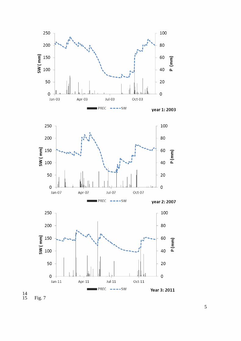
Taking into account all these observations and the different rainfall patterns recorded in the area, 190

a simulation of climate change effects on soil erosion was carried out for three years with different 191

rainfall characteristics. The selected years were 2003 (year 1), 2007 (year 2) and 2011 (year 3). The 192

rainfall distribution of these years is presented in Fig. 6. Year 1 and year 2 recorded similar amounts of 193

total precipitation which was close to the average in the area. Rainfall was mainly concentrated in spring 194

and autumn, but with different annual distributions and patterns of rainfall intensity. In year 1, 195

precipitation was greater in spring than in autumn, while the opposite was observed in year 2. Year 3 was 196

the wettest year, with precipitation more homogeneously distributed throughout the year and with 2 197

extreme events that each recorded more than 70mm.Year 3 may be a good example of a situation which is 198

occurring with greater frequency, namely an increasing number of extreme events which make a 199

significant contribution to the amount of annual rainfall. Additionally, based on the observed trends of 200

rainfall intensity, the influence of 10% and 20% increases in rainfall intensity wasevaluated for the 2020 201

and 2050 scenarios. The effects of the changes of different variables (temperature, solar radiation, 202

humidity and precipitation) were simultaneously analysed. In addition, the variations in rainfall intensity 203

were considered. 204

205

206

9

3 Results 207

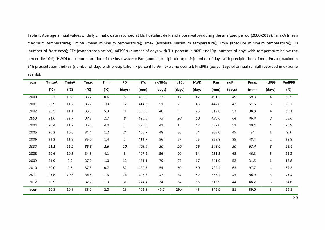
3.1 Climatic characteristics 208

Table 4 shows the average values of various annual temperature and precipitation variables for the period 209

2000-2012. Temperature variables included mean maximum (TmaxA) and minimum temperature 210

(TminA), maximum (Tmax) and minimum temperature (Tmin), as well as some parameters related to 211

extremes such as number offrost days (FD), number of days with temperature > percentile 90% (ndT90p) 212

and < percentile 10% (nd10p) and duration of heat waves (HWDI). Precipitation variables refer to total 213

annual precipitation (Pan), number of rainy days (ndP),maximum 24h rainfall (Pmax) and number of 214

extreme events (events that recorded P>95percentile) (nd95), as well as the precipitation that these events 215

represented in relation to annual precipitation (PndP95). Mean annual temperature ranged between 20.0 216

and 21.9 ºC, while mean minimum temperature ranged between 9.3 and 11.9 ºC. This period included 217

some of the warmest years recorded in recent decades, with a mean maximum temperature about 1.3 ºC 218

higher than in the period 1970-2000 (Camps and Ramos, 2012) and a corresponding difference in 219

minimum temperature of about 1.39 ºC. Other indices were also higher, including the length of heat 220

waves (average value of 45 days vs. 32.7 days and with a longest period of 67 days) and the number of 221

days with temperature > 90percentile (50 vs. 31.1 days). Annual evapotranspiration increased at a ratio of 222

about 1.125 mm per year during the period analysed, whereas the ratio of change in the period 1970-2000 223

was 0.649 mm per year. These results therefore help to illustrate the potential effects of climate change in 224

the area, despite the high degree of variability from year to year. 225

In relation to precipitation, average annual precipitation was about 550 mm during the period 226

2000-2012, ranging from 329.8 mm to 751.5 mm and mainly distributed in spring and autumn. This value 227

did not differ significantly from the average in the area related to longer periods (Camps and Ramos, 228

2012). The number of rainy days (P > 1mm) ranged between 35 and 68 and maximum 24h rainfall 229

between 31.5 and 97.7 mm. The number of events with precipitation greater than that corresponding to 230

the 95% percentile (extreme events) ranged between 1 and 5, and precipitation recorded in those events 231

represented between 9.3 and 41.4% of annual rainfall. 232

Regarding the three years selected for the simulation (2003, 2007 and 2011), maximum 233

precipitation in 24h differed considerably (46.4, 68.4 and 86.9 mm, respectively) and the number of days 234

with precipitation greater than 1 mm was 64, 50 and 45, respectively (Table 4). The number of days on 235

10

which precipitation was greater than the 95% percentile (extreme events) was 3 in each of the three years, 236

but represented respectively 38.6, 26.4 and 41.4% of annual rainfall. Maximum rainfall intensity in 30 237

minutes recorded during these years ranged between 9.2 and 10.4 mm h-1

. 238

239

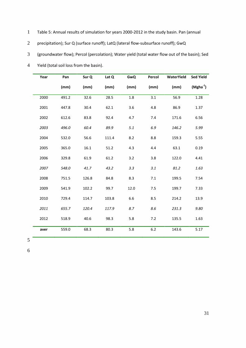
3.2 Runoff rates and soil loss 240

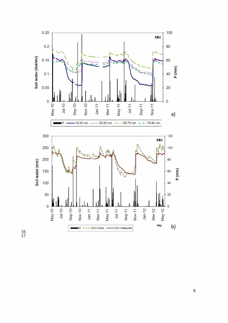
Table 5 shows the results of annual simulations for the years 2000 to 2012 (the years 1998 and 1999 were 241

used as SWAT warm-up period). Due to the soil characteristics, a significant amount of rainfall infiltrated 242

the soil profile, but then moved as subsurface flow (Lat Q). This represented between 5.4 and 19.2% of 243

annual rainfall. This result was subsequently confirmed in the field by soil water content measurements. 244

Figure 7a shows the evolution of soil water content in the soil profile during a 2 year period in the SB2 245

subbasin and total soil water in the profile measured and simulated by the model is shown in Fig. 7b. It 246

can be observed that soil water did not significantly change after some rainfall events (particularly after 247

those of high intensity). In addition, soil water did not change homogeneously in the whole profile due to 248

differences in soil properties between layers. However, average soil water content in the soil was 249

relatively well simulated by the model. For the period analysed, runoff (Sur Q) varied from year to year, 250

with values ranging between 16.1 and 126.8 mm. This represented between 4.4 and 18.8% of total annual 251

rainfall, with an average ratio of about 12%. Runoff rates represented between 25.5 and 63.5% of water 252

yield with large differences between dry and wet years. Sediment yield ranged between less than 1 and 253

13.9 Mg ha-1

yr-1

, with an average value of 5.2 Mg ha-1

yr-1

. 254

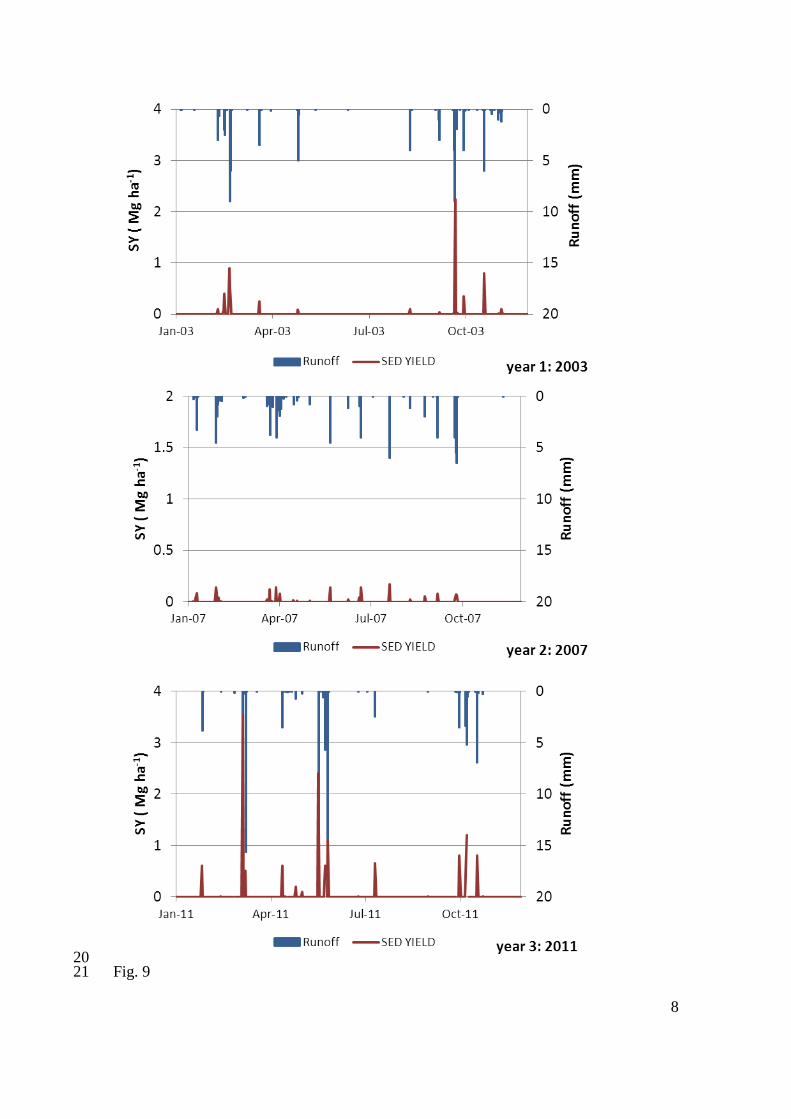
As expected, high differences in soil erosion were observed between the three representative 255

years (year 1: 2003; year 2: 2007 and year 3: 2011). Figure 8 shows runoff and soil losses simulated for 256

the three years in one of the subbasins (SB2). The differences in rainfall distribution produced differences 257

in initial soil water conditions which influence runoff rates. Sediment yield in year 1 was estimated at 258

5.99 Mg ha-1

yr-1

, (similar to the average value for the area), while in year 2 soil loss was estimated at 1.6 259

Mg ha-1

yr-1

and in year 3 at 9.8 Mg ha-1

yr-1

. The differences in the response can be attributed to the 260

rainfall characteristics and the initial soil water conditions (Fig. 7). It can be seen that in 2003 and 2011, 261

most soil loss was recorded in a small number of events, which were separated by long dry periods. In 262

2003, the rainfall events that generated higher soil loss were recorded in autumn, while in 2011 the main 263

erosive events were recorded in spring. 264

11

Nevertheless, erosion rates in some parts of the basin, particularly in areas close to the basin 265

outlet cultivated with vines, may be much higher than the simulated average for the analysed years. 266

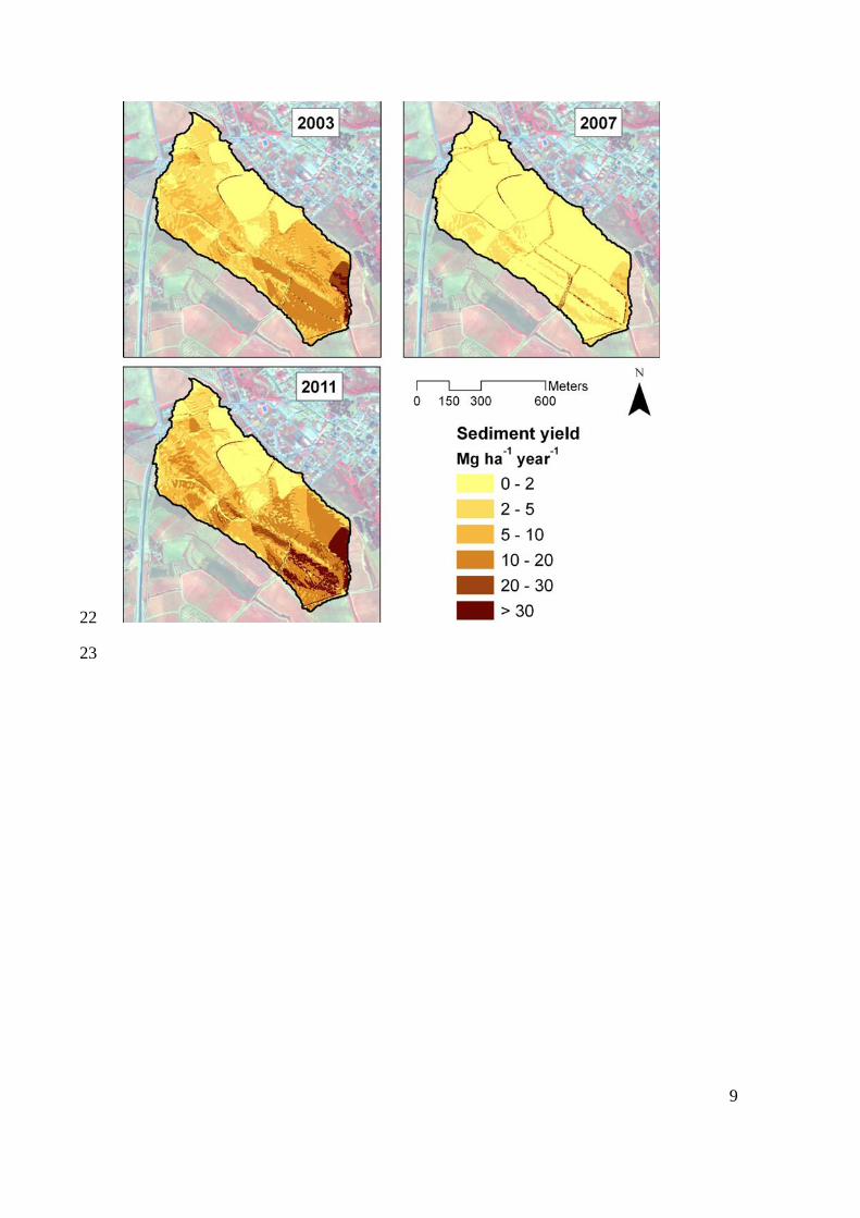
Figure 9 shows the distribution of soil losses simulated in the basin for the three selected years. For 2003 267

and 2011, in which higher erosion rates were simulated, soil losses in vineyards were higher than 10 Mg 268

ha-1

in many areas, while for other crops like olive trees, winter barley or alfalfa, soil losses were below 5 269

Mg ha-1

. These values were confirmed for 2011 which was included in the model calibration (Ramos and 270

Martínez-Casasnovas, 2014). 271

272

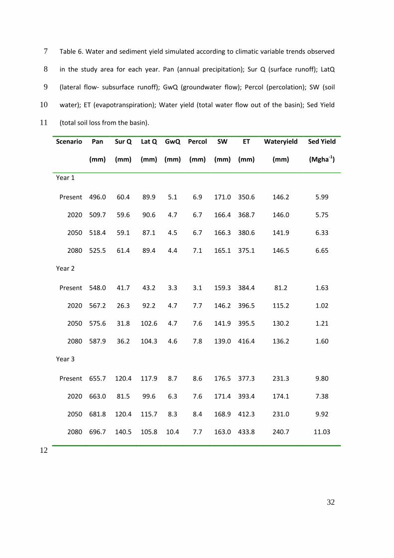
3.3 The influence of climate change on soil loss 273

The results of the simulation for the projected rainfall distributions (2020, 2050 and 2080 scenarios) were 274

compared with those obtained for the present situation in Table 6. The model responded to increased 275

precipitation by generating an increase in runoff and sediment yields. However, in the first step, when all 276

the variables except rainfall intensity were changed, for the 2020 scenario, the increase in temperature 277

gave rise to an increase in evapotranspiration and a decrease in soil water content.Precipitation rose only 278

slightly,which was not enough to balance the increase in evapotranspiration. The result was a decrease in 279

runoff and soil loss was lower than at present. However, for the 2050 scenario, the small change in 280

precipitation was enough to offset the increase in evapotranspiration. In that case, runoff increased as did 281

soil loss. Soil loss would be up to 5.6% greater than at present for 2050 and about 12% greater for 2080 in 282

years with higher autumn rainfall precipitation and extreme events (years 1 and 3). In year 1 and year 3, 283

despite the differences in total soil erosion, the change ratios moved in the same direction. However, no 284

significant differences were found for year 2, for which soil losses were low. 285

Nevertheless, it should be underlined that the main changes in soil loss appeared when rainfall 286

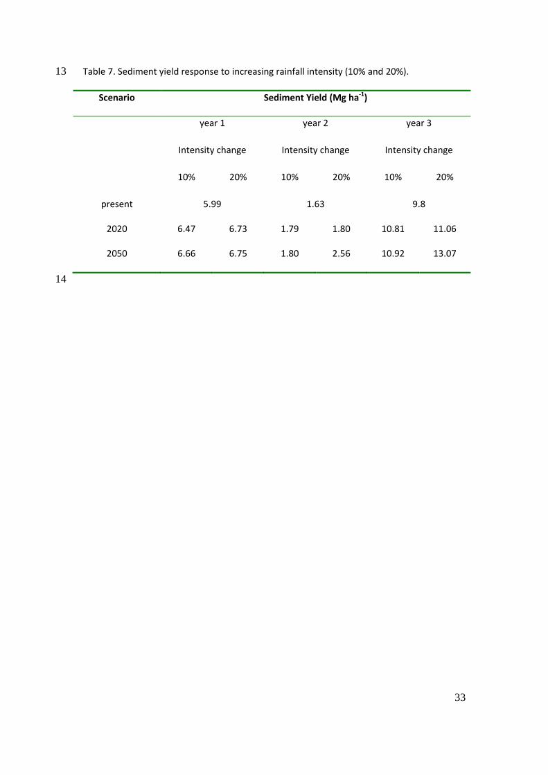
intensity varied. For the same rainfall distribution, a 10% increase in intensity in year 1 produced an 287

increase in soil loss of between 8 and 10% for the 2020 scenario and of between 10 and 13% for the 2050 288

scenario. An increase in intensity of 20% could therefore increase soil loss by up to 57% for the 2050 289

scenario (Table 7). For year 2, although erosion rates were lower, the change ratios for the 2050 scenario 290

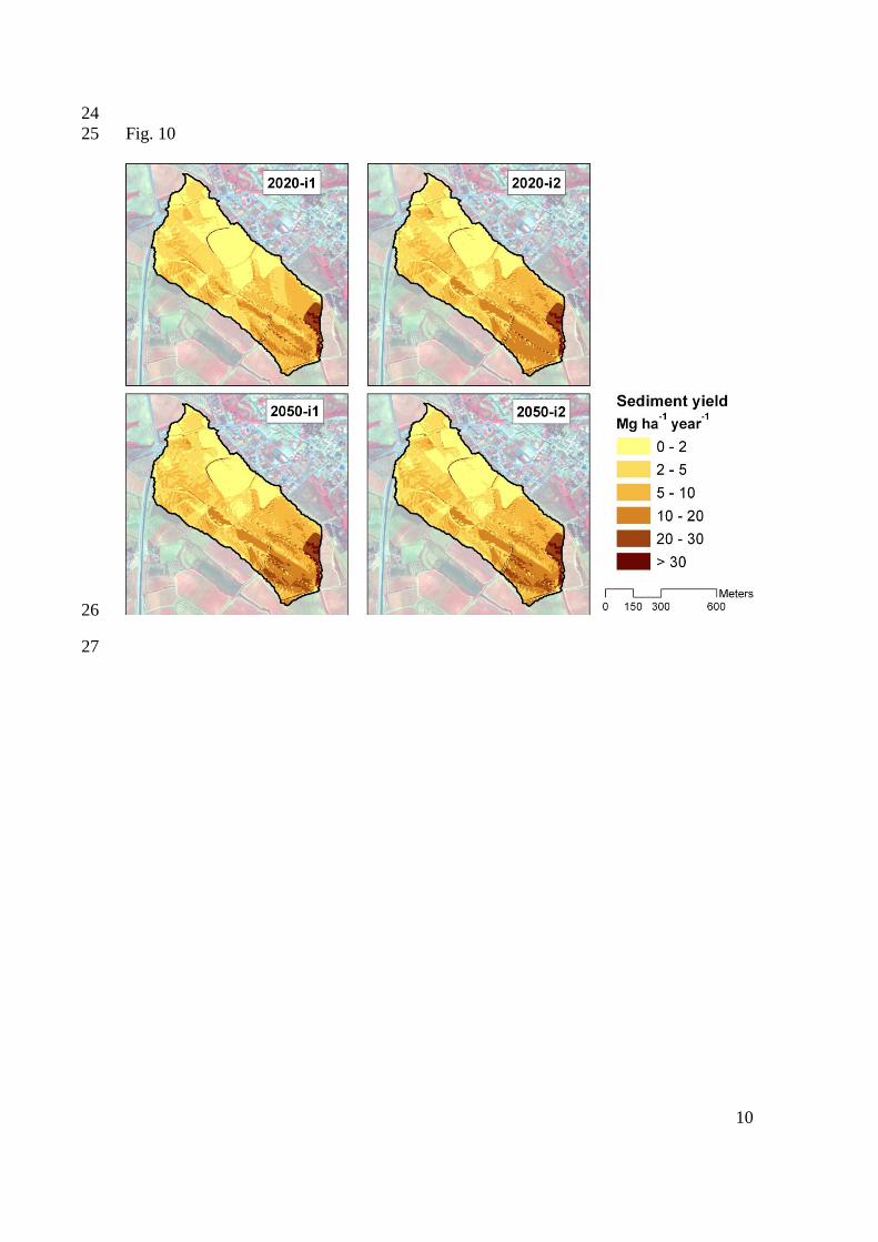
were the highest. Figure 10 illustrates the changes in soil loss within the basin simulated for the 2020 and 291

2050 scenarios as well as changes in rainfall intensity. 292

293

12

294

4 Discussion 295

For the period analysed (2000-2012), the simulation that was undertaken gave high runoff rates not only 296

in wet years but also in relatively dry or normal years, like 2006 and 2009. These high annual runoff rates 297

were usually due to a low number of rainfall events, which were mainly recorded in autumn and the rates 298

were of the same order of magnitude as those reported by other authors for Europe and the Mediterranean 299

area. In this respect, Maetens et al. (2012) cited runoff rates of 5-10% in a study comprising 227 plot-300

measuring sites. 301

The simulated soil loss presented high variability from year to year, depending on rainfall 302

characteristics. Nevertheless, in most of the years the values represent a soil threat, as soil losses over 1 or 303

2 Mg ha-1

yr-1

are irreversible (Panagos and Montaranella, 2014). Within the basin, the highest erosion 304

rates occurred in the areas near the basin outlet, or where the soil had been highly disturbed by levelling 305

operations before vineyard establishment. The erosion rates obtained for the study area were in line with 306

those observed in other research works relating to vines grown in the Mediterranean area. Kosmas et al. 307

(1997) reported soil losses of between 0.67 and 4.6 Mg ha-1

yr-1

in different Mediterranean countries 308

(Portugal, Spain, France, Italy and Greece). Ruiz Colmenero et al. (2013) found soil losses of 5.88 Mg ha-309

1yr

-1 in vineyards with traditional management, although Bienes et al. (2012) reported soil losses of up to 310

20 Mg ha-1

yr-1

in the same areas. In the area where the study basin was located, higher erosion rates were 311

also measured at plot scale; for example, losses of up to 18-22 Mg ha-1

were measured after a period of 312

high intensity autumn rainfall (Ramos and Porta, 1997). Other results in the same area have shown 313

erosion rates of between 15 and 25 Mg ha-1

yr-1

in vineyard plots that had been previously levelled (Ramos 314

and Martínez-Casasnovas, 2010). Similarly, for vineyards with bare soil, Maetens et al. (2012) found soil 315

losses of 10-20 Mg ha-1

yr-1

. Other studies have cited even higher erosion rates: 7-21 Mg ha-1

yr-1

in 316

Alsatian vineyards (Schwing, 1978); up to 35 Mg ha-1

yr-1

in the mid-Aisne region of France (Wicherek, 317

1991); and 8-36 Mg ha-1

yr-1

in the Languedoc region of France (Paroissien et al., 2010). 318

The high variability observed from year to year makes it difficult to draw conclusions about the 319

influence of temperature and precipitation changes on erosion rates. It can, however, be seen that four of 320

the five years with the highest simulated soil losses (similar to or greater than 7.5 Mg ha-1

yr-1

) were 321

recorded in the period 2008-2011. The increasing soil losses (simulated as well as observed) is in 322

13

agreement with the increasing tendency for extreme events referred to by other authors (Kharin et al., 323

2007; Ramos and Martínez-Casasnovas, 2009) and provides information about the impact of climate 324

change on soil erosion processes. 325

The model was run at daily scale, which may not reproduce well the changes in precipitation and 326

intensity. Even so, by modifying the monthly maximum rainfall intensity it was possible to obtain an idea 327

of the influence of climate change on soil erosion. For the years analysed, an increase of 10% in rainfall 328

intensity, which has already been observed in the area, increased soil loss by between 8 and 10.3% for the 329

2020 scenario, and by up to 57% for the 2050 scenario. This implies that by 2050 the impact of increasing 330

rainfall intensity on soil erosion could be much more severe than at present, particularly when extreme 331

and highly erosive events are increasing (Ramos and Durán, 2014). These results agree with predictions 332

made for other areas. O’Neal et al. (2005) predicted an increase in soil losses ranging between 37 and 333

274% for the period 2040-2059 in the US Mid-West, with projected runoff rates increasing by between 10 334

and 31%. Similarly, Zhang et al. (2012), projected mean annual runoff and soil loss increases in 335

rangeland in South-eastern Arizona ranging from 79% to 92% and from 127% to 157%, respectively, 336

relative to the period 1970-1999. In Europe, van der Velde et al. (2014) simulated changes in erosion 337

rates from 14.4 to 19.1 Mg ha−1

and from 9.1 to 9.7 Mg ha-1

, for 1981-2010 and 2071-2100, respectively, 338

based on the reference climate data (CNTRL) and on climate data with reduced variability (REDVAR). 339

Märker et al. (2008) for Tuscany (Italy) indicated thateven with a decline in precipitation volume until 340

2070, higher erosion rates may occur in some months due to higher rainfall erosivity. However, other 341

predictions indicate that soil erosion could decrease with climate change depending on local 342

climatological and environmental conditions (Dabson et al., 2010; Scholz et al., 2008). Dabson et al. 343

(2010) predicted an increase in soil erosion in northern Europe by 2080, but a probable decrease for 344

southern Europe. However, Scholz et al. (2008) predicted a decline in annual average soil losses from 345

sugar beet cultivation in Central Europe in response to climate change. Nevertheless, the work of these 346

authors highlights the importance of seasonal changes in climatic parameters for the discussion about the 347

impacts of global climate change on future soil erosion rates. 348

Apart from temperature changes, one of the main threats in Mediterranean environments will be 349

the greater irregularity of rainfall distribution throughout the year. It can be seen that most soil loss in 350

2003 and 2011 was recorded in a small number of events which were separated by long dry periods. In 351

2003, the rainfall events that generated the highest soil loss were recorded in autumn, while in 2011 the 352

14

main erosive events were recorded in spring. This is one of the main changes that may become more 353

frequently observed in the study area. While spring rainfall used to be of low intensity, during recent 354

years the number of erosive events of high intensity has increased (Ramos and Durán, 2014). Longer dry 355

periods and greater rainfall concentration in a reduced number of events of higher intensity may affect the 356

risk of erosion. More extensive droughts can remove the protective vegetation cover leaving the soil more 357

exposed to erosion, while more intensive rains can detach more soil and produce a severe increase in 358

erosion rates. 359

360 Although the results obtained with the simulations only refer to a relatively small basin area, this 361

area is representative of the land use and landscape of the region and could give a good idea of the 362

response of this kind of agricultural system to climate change impacts. The crops cultivated in the study 363

basin are associated with high erosion rates due to the scarce soil cover; because of this, these are the soils 364

that could suffer the greatest increases in soil losses as a result of climate change. The simulated results 365

show that, under the scenarios analysed in the present study, the soil loss tolerance threshold may be 366

exceeded not only in some parts of the basin, as at present, but in most of the vineyards within the basin. 367

This increase of soil erosion may affect the sustainability of this agricultural system under Mediterranean 368

climate conditions and the management practices used in the area. The results highlight the need to 369

establish conservation measures to reduce soil losses and maintain the sustainability of this agricultural 370

system. 371

372

373

5 Conclusions 374

The results of this research confirm the difficulties of extracting accurate predictions of the influence of 375

climate change on soil erosion in the Mediterranean area. High variability in soil loss was predicted from 376

year to year. This variability was associated with differences in total precipitation which were greater than 377

would normally be expected under a climate change scenario. Furthermore, high intensity events over 378

short time periods were not well represented. 379

The SWAT model responds to the amount of rainfall and to changes in temperature which, in 380

turn, influence evaporation rates. However, in the analysed period, in which the changes in precipitation 381

were mainly changes in the distribution and intensity of rainfall, but not in total amount, some difficulties 382

15

arose when trying to make suitable predictions. In order to obtain understandable results, it was necessary 383

to take into account changes in rainfall intensity in combination with changes in other climatic variables. 384

This is because soil losses depend on runoff and this, in turn, on the soil-water-plant interaction and 385

vegetation growth which is also influenced by temperature. 386

This modelling application also allowed us to estimate the increase in soil erosion that vineyards 387

may suffer in the study area as a consequence of changes in climatic variables. It was confirmed that an 388

increase in the intensity of erosive events, similar to that observed during recent years (between 10 and 389

20%) may give rise to an increase in soil loss of between 8 and 10.3% for the 2020 scenario and up to 390

57% for the 2050 scenario. These figures should be taken into account by regional planners to reorient 391

land uses and/or management practices to avoid further land degradation. 392

393

394

Acknowledgements This work is part of research project AGL2009-08353 funded by the Spanish 395

Ministry of Science and Innovation. We would like to thank the Castell d’Age winery for their support 396

and for allowing us to carry out field experiments on their property. 397

398

16

References 399

Bagnold RA (1977) Bed load transport by natural rivers. Water Resources Research13: 400

303-312. 401

Bang HQ, Quan NH,Phu VL (2013) Impacts of Climate Change on Catchment Flows 402

and Assessing Its Impacts on Hydropower in Vietnam’s Central Highland Region. 403

Global Perspectives on Geography 1(1): 1-8. 404

Bienes R, Marqués MJ,Ruíz-Colmenero M (2012)Herbaceous crops, vineyards and 405

olive groves. The traditional land management and its impact on water erosion. 406

Cuadernos de InvestigaciónGeográfica 38 (1): 49-74 407

Camps JO, Ramos MC (2012) Grape harvest and yield responses to inter-annual 408

changes in temperature and precipitation in an area of north-east Spain with a 409

Mediterranean climate. International Journal of Biometeorology 56: 853-864. 410

Dadson S, Irvine B, Kirkby M (2010) Effects of climate change on soil erosion: 411

Estimates using newly-available regional climate model data at a pan-European 412

scale. GeophysicalResearchAbstract 12, EGU2010-7047. 413

DAR (2008) Mapa de Sòls (1:25.000) de l’àmbit geogràfic de la 414

Denominaciód’OrigenPenedès. Departamentd’Agricultura, Alimentació i Acció 415

Rural, Generalitat de Catalunya, Vilafranca del Penedès-Lleida. 416

Easterling DR, Meehl GA,Parmensan C, Chagnon SA, Kart T,Mearns LO (2000) 417

Climate extremes: observation, modelling and impacts. Science 289: 2068-2074. 418

Favis-Mortlock DT, Boardman J (1995) Nonlinear responses of soil erosion to climate 419

change: a modelling study on the UK South Downs. Catena 25: 365-387. 420

González-Hidalgo JC, Brunetti M, de Luis M (2010)Precipitation trends in Spanish 421

hydrological divisions, 1946-2005. Climate Research 43(3): 215–228. 422

17

Gupta HV, SorooshianS,Yapo PO (1999). Status of automatic calibration for hydrologic 423

models: Comparison with multilevel expert calibration. Journal of Hydrologic 424

Engineering 4(2): 135-143. 425

Hirschi M,Seneviratne SI (2010) Intra-annual link of spring and autumn precipitation 426

over France. Climate Dynamics 35 (7): 1207-1218. 427

Iowa Learning Farms - Iowa State University 2103. The cost of erosion. 428

http://www.extension.iastate.edu/ilf/sites/www.extension.iastate.edu/files/ilf/Cost429

_of_Eroded_Soil.pdf 430

Jentsch MF, James PAD, Bahaj AS (2012) Climate change world weather file 431

generator. Sustainable Energy Research Group. University of Southampton. 432

http://www.serg.soton.ac.uk/ccworldweathergen/ 433

Kharin VV, Zwiers FW, Zhang X, Hegerl GC (2007) Changes in temperature and 434

precipitation extremes in the IPCC ensemble of global coupled model simulations. 435

Journal of Climate 20: 1419–1444 436

Klein Tank AMG,Können GP (2003) Trends in Indices of Daily Temperature and 437

Precipitation Extremes in Europe, 1946–99. Journal of Climate 16: 3665–3680. 438

Kosmas C N, DanalatosLH,Cammeraat M, Chabart J, Diamantopoulos R, Farand L, 439

Gutierrez A, Jacob H, Marques J, Martinez-Fernandez A, Mizara N, Moustakas 440

JM, Nicolau C, Oliveros G, Pinna R,Puddu J,Puigdefabregas M, Roxo A, Simao 441

G, StamouMn, Tomasi D, Usai D, Vacca A (1997) The effect of land use on 442

runoff and soil erosion rates under Mediterranean conditions. Catena 29:45-59. 443

Maetens W, Vanmaercke M, Poesen J, Jankauskas B, Jankauskiene G, Ionita, I (2012) 444

Effects of land use on annual runoff and soil loss in Europe and the 445

Mediterranean: A meta-analysis of plot data. Progress in Physical Geography 446

36(5): 599-653. 447

18

Märker M, Angeli L,Bottai L, Costantini R, Ferrari R, Innocenti L, Siciliano G (2008) 448

Assessment of Land Degradation Susceptibility by Scenario Analysis: A Case 449

Study in Southern Tuscany, Italy, Geomorphology 93, (1–2).120-129. 450

Martínez-Casasnovas JA, Ramos MC (2009)Soil alteration due to erosion, ploughing 451

and levelling of vineyards in north east Spain. Soil Use and Management25: 183- 452

192. 453

Martínez-Casasnovas JA (2003) A spatial information technology approach for the 454

mapping and quantification of gully erosion. Catena 50: 293-308. 455

Martínez-Casasnovas JA, Ramos MC (2006) The cost of soil erosion in vineyard fields 456

in the Penedès–Anoia Region (NE Spain). Catena 68: 194-199. 457

Moriasi DN, Arnold JG, Van Liew MW, Bingner RL, Harmel RD,Veith TL (2007) 458

Model evaluation guidelines for systematic quantification of accuracy in 459

watershed simulations. Transactions of the ASABE 50:885-900. 460

Mukundan R, Pradhanang SM, Schneiderman E M, Pierson DC, Anandhi A, Zion M 461

S, Matonse AH, Lounsbury DG,Steenhuis TS (2013). Suspended sediment source 462

areas and future climate impact on soil erosion and sediment yield in a New York 463

City water supply watershed, USA. Geomorphology 183 (1): 110–119. 464

Nash JE, Sutcliffe JE (1970) River flow forecasting through conceptual models. Part 1. 465

A discussion of principles. Journal of Hydrology 10 (3): 282–290. 466

Nearing MA, Jetten V, Baffaut C, Cerdan O, Couturier A, Hernandez M, Le Bissonnais 467

Y, Nichols MH, Nunes JP, Renschler CS, Souchère V, van Oost K 468

(2005)Modeling response of soil erosion and runoff to changes in precipitation 469

and cover. Catena 61: 131-154. 470

Neitsch SL, Arnold JG, Kiniry JR, Williams JR (2011) Soil and Water Assessment 471

Tool: Theoretical Documentation Version 2009. Texas Water Resources Institute 472

19

technical Report No. 406. College Station, Texas, USA: Texas A&M University 473

System. Available online from: http://twri.tamu.edu/reports/2011/tr406.pdf 474

(accessed March 2014). 475

Nunes JP, Nearing MA (2011) Modelling Impacts of Climatic Change: Case Studies 476

using the New Generation of Erosion Models. In R.P.C Morgan and M.A. 477

Nearing. (Eds) Handbook of Erosion Modelling. Blackwell Publishing Ltd. 478

O’Neal MR, Nearing MA, Vining RC, Southworth J, Pfeifer RA (2005) Climate change 479

impacts on soil erosion in Midwest United States with changes in crop 480

management. Catena 61: 165–184. 481

Panagos P,Montanarella L (2014). What is the Cost of Soil Erosion inEurope?. 20th 482

World Congress of Soil Science. Joint Research Centre 483

(JRC).http://eusoils.jrc.ec.europa.eu/events/Conferences/20WCSS/Presentations/S484

oil_ErosionCOST.pdf 485

Paroissien J, Lagacherie P, Le Bissonnais Y (2010) A regional-scale study of multi-486

decennial erosion of vineyard fields using vine-stock unearthing–burying 487

measurements. Catena 82:159-168. 488

Ramos MC, Martínez-Casasnovas JA (2009) Impacts of annual precipitation extremes 489

on soil and nutrient losses in vineyards of NE Spain. Hydrological Processes 23: 490

224–235. 491

Ramos MC, Martínez-Casasnovas JA(2010)Effectsoffieldreorganisationonthespatial 492

variability ofrunoffanderosion rates in vineyardsofNortheastern Spain. Land 493

DegradationandDevelopment, 21: 1-15. 494

Ramos MC, Balash JC,Martínez-Casasnovas JA (2012) Seasonal temperature and 495

precipitation variability during the last 60 years in a Mediterranean climate area of 496

20

Northeastern Spain: a multivariate analysis. Theoretical Applied Climatology 497

110:35-53 498

Ramos MC,Martínez-Casasnovas JA (2014)Soil water content, runoff and soil loss 499

prediction in a small ungauged agricultural catchment in the Mediterranean region 500

using the Soil and Water Assessment Tool. Journal of Agricultural Science, (on 501

line) doi:10.1017/S0021859614000422. 502

Ramos MC, Durán B (2014)Assessment of rainfall erosivity and its spatial and temporal 503

variabilities: Case study of the Penedès area (NE Spain). Catena, 123: 135-504

147Ramos MC, PortaJ (1997) Analysis of design criteria for vineyard terraces in 505

Mediterranean area of North East Spain.Soil Technology10, 155-166. 506

Ruiz-Colmenero M, Bienes R, Eldridge DJ, Marques MJ (2013) Vegetation cover 507

reduces erosion and enhances soil organic carbon in a vineyard in the central 508

Spain. Catena 104, 153-160. 509

Schwing JF (1978) L'erosion des sols dans le vignoble alsacien, son importance et son 510

evolution en fonction des techniques agricoles. Catena 5:305-319. 511

Scholz G, Quinton JN, Strauss P ( 2008) Soil Erosion from Sugar Beet in Central 512

Europe in Response to Climate Change Induced Seasonal Precipitation Variations. 513

Catena 72,(1), 91-105. 514

USDA-SCS (1985) National Engineering Handbook, Section 4 - Hydrology. 515

Washington, D.C.: USDA-SCS. 516

van der Velde M, Balkovič J, Beer C, Khabarov N, Kuhnert M, Obersteiner M, Skalský 517

R, Xiong W, Smith P (2014) Future climate variability impacts on potential 518

erosion and soil organic carbon in European croplands, Biogeosciences Discuss., 519

11, 1561-1585. 520

21

Viatcheslav KV, Zwiers FW, Zhang X, Hegerl CG (2007)Changes in Temperature and 521

Precipitation Extremes in the IPCC Ensemble of Global Coupled Model 522

Simulations. Journal of Climate 20: 1419–1444. 523

Wicherek S (1991) Viticulture and soil erosion in the north of Parisian Basin. Example: 524

the mid Aisne region. Zeitschrift fur Geomorphologie, Supplementband 83:115-525

126. 526

Williams J R, Berndt H D (1977) Sediment yield prediction based on watershed 527

hydrology. Transactions of the ASAE 20: 1100-1104. 528

Wischmeier WH, Johnson CB, Cross BV (1971) A Soil erodibilitynomograph for 529

farmland and construction sites. Journal of Soil and Water Conservation 26: 189-530

193 531

Zhang Y, Hernandez M, Anson E, Nearing MA, Wei H, Stone JJ,Heilman P 532

(2012)Modeling climate change effects on runoff and soil erosion in southeastern 533

Arizona rangelands and implications for mitigation with conservation practices. 534

Journal of Soil and Water Conservation 67 (5): 390-405 535

536

22

Figure captions 537

Fig. 1. Location of the study area 538

Fig. 2. Land uses in the basin and location of the subbasins in which model 539

calibration and validation were carried out. 540

Fig. 3 a) Comparison between simulated Tmax and Tmin and those extrapolated from 541

the observations in the study area between 1960 and 2012, for the 2020 scenario. b) 542

Changes in maximum and c) minimum temperature simulated for the 2020, 2050 and 543

2080 scenarios. 544

Fig. 4 a) Change of relative humidity and b) global solar radiation simulated with the 545

CCWorldWeatherGen model for the 2020, 2050 and 2080 scenarios. 546

Fig. 5. Trends of 30-min maximum rainfall intensity recorded between 1994 and 2013 547

at Els Hostalest de Pierola (EHP) and Vilafranca del Penedès (VP). 548

Fig. 6. Rainfall distribution and soil water content of the selected years. 549

Fig. 7 a) Soil moisture measurements at different depths in subbasin SB2 and b) 550

Comparison between average measured and simulated soil water in the profile. 551

Fig. 8. Soil loss and runoff simulated for the three selected years. 552

Fig. 9. Soil loss distribution within the basin for the three selected years under present 553

conditions. 554

Fig. 10. Soil loss distribution within the basin for year 1 under the 2020 and 2050 555

scenarios, with increasing changes in rainfall intensity.556

23

Fig. 1 557

558 559

24

560

Fig. 2 561

562

563 564

565

2

Fig. 3 1

2

2

Fig. 4 1

2

3 4

5

6

3

7

Fig. 8

59

10 11

4

12

Fig. 6 13

5

14 Fig. 7 15

6

16 17

7

18

Fig. 8 19

8

20 Fig. 9 21

9

22

23

10

24

Fig. 10 25

26

27

27

Table 1: Average monthly values and standard deviation of climatic data recorded in Els Hostalest de Pierola (period 1998-2012): TMaxM (average maximum

air temperature ± standard deviation for month); TminM (average minimum air temperature ± standard deviation for month); PPM (average amount ±

standard deviation of rainfall falling in month; ndPM (average number of days with precipitation in month); RIHHmax (extreme half-hour rain per month);

WINM (average wind speed ± standard deviation in month); SRM (average solar radiation ± standard deviation per month); RH (average relative humidity).

variable Jan Feb Mar Apr May Jun Jul Aug Sep Oct Nov Dec

TmaxM (°C) 12.8±3.1 15.3±2.4 18.4±1.8 20.2±1.5 24.9±2.1 29.4±1.7 31.4±1.7 31.3±2.1 26.1±4.4 22.8±1.5 16.4±1.8 13.2±1.8

TminM(°C) 3.5±1.3 4.2±1.6 6.3±1.2 7.9±1.1 12.1±1.3 16.0±0.9 18.2±0.9 18.2±1.3 16.1±2.4 12±1.1 6.1±1.9 3.9±1.7

PPM (mm) 32.9±38.7 30.2±37.2 40.5±33.6 58.1±47.2 56 42.4 38.4±32.4 18.6±16.5 46.0±32.1 40.2±29.9 89.3±38.2 45.92.7±43.1 30.3±29.6

ndPM 6 6.9 8.7 10.2 10.4 6.67 5.8 7.1 8 9.6 5.82 7.3

RIHHmax(mmh-1

) 14.4 7.7 11 10 10.8 50.8 36.8 42.1 44 30.4 30.9 10.5

WINM (ms-1

) 2.3±0.6 2.5±0.5 2.7±0.6 2.8±0.9 2.3±0.5 5.2±0.7 2.5±0.6 4.9±0.6 4.7±0.6 1.9±0.5 2.2±0.6 4.76±0.5

SRM (Jm-2

) 4.7±1.8 6.3±2.7 9.5±3.7 10.9±4.0 143.9±5.9 16.1±7.0 14.9±5.6 13.3±5.2 10.4±4.0 8.8±4.4 6.2±3.1 4.6±2.0

RH (%) 74.4±5.6 67.3±7.7 66.2±5.9 65.9±5.3 63.8±4.2 57.1±12.1 61.7±4.8 63.7±9.0 70.6±7.3 74.3±7.9 74.5±9.1 75.6±7.7

28

Table 2. Mean values and standard deviation (m±std) of soil properties of the most representative soils in the study basin: root depth, lower boundary depth

of each horizon (SDH), texture fraction (clay, silt, sand- USDA), coarse elements, organic carbon (OC), electrical conductivity (EC), bulk density (BD), available

water capacity (AWC= water retention capacity at 33kPa - water retention capacity at -1500kPa), steady infiltration rate (StIR); K-erodibility USLE factor (K-

factor).

SOIL series

Root depth

(mm)

SDH (mm)

(m±std)

Finefraction (< 2mm)

Coarse elem. fraction of total

soil (%)

(m±std)

OC (%)

(m±std)

EC (dS m

-1 )

(m±std)

BD (kg m

-3)

(m±std)

AWC (%)

(m±std)

StIR (mm h

-1)

(m±std)

K-factor (Mg ha h ha

-1MJ

-1mm

-1)

(m±std) Clay (%)

(m±std)

Silt (%)

(m±std)

Sand (%)

(m±std)

S1 800 240 10.9±4.4 20.1±3.0 68.1±2.5 25.2±2.0 1.1±0.3 0.14±0.01 1754±320 10.8±0.3 27.2±2.3 0.043±0.08

Falguerar 620 14±2.6 37±5.4 48±1.9 25.0±1.8 0.2±0.1 0.19±0.01 1953±280 13.1±0.4 0.055

1380 28±4.1 39±4.1 33±1.7 5.0±1.1 0.1±0.1 0.16±0.01 1810±300 14.2±0.8 0.040

S2 1000 330 19.0±4.1 40±4.3 41±4.2 44.0±2.0 0.7±0.18 0.10±0.01 1638±160 13.7±0.5 8.2±1.2 0.037±0.07

Pierola 670 13.3±2.7 24.1±2.8 62.5±3.8 72.0±2.8 0.3±0.1 0.10±0.01 1725±231 13.1±1.2 0.030

1000 6.6±2.3 2.3±2.5 91.1±4.1 71.0±3.8 0.2±0.1 0.20±0.01 1920±285 12.5±1.1 0.020

S3 1000 330 20.0±4.7 30±3.2 50±2.9 25.0±1.9 1.4±0.2 0.10±0.01 1750±320 9.6±1.0 12.2±0.5 0.045±0.06

Marquet 670 13.3±3.1 24.1±2.8 62.5±2.8 72.0±4.3 0.3±0.1 0.10±0.01 1710±295 13.1±1.7 0.030

1000 6.6±2.5 2.3±1.1 91.1±3.8 71.0±5.1 0.2±0.1 0.20±0.01 1920±350 12.5±1.5 0.020

S4 1670 240 20.1±3.1 43.5±3.7 36.4±2.1 23.6±2.8 1.53±0.13 0.14±0.01 1350±220 8 1±1.1 8.2±2.0 0.045±0.07

Hostalets 540 14±2.2 38±2.8 48±1.9 50.0±3.2 0.6±0.2 0.18±0.01 1451±230 7.8±1.9 0.047

860 15±2.3 42±3.0 43±2.0 50.0±2.8 0.3±0.1 0.19±0.01 1530±290 2±0.5 0.043

S5 800 240 19.3±2.6 27.4±2.6 53.3±4.2 17.5±1.8 1.29±0.12 0.16±0.01 1900±310 8.0±0.5 10.0±1.0 0.038±0.05

Cabanyes 550 16.5±2.3 52±3.3 31.5±2.6 35.0±2.5 0.6±0.2 0.17±0.01 1498±250 13.1±0.8 0.041

800 18.5±2.5 32.5±4.0 49±2.9 35.0±2.8 0.1±0.1 0.19±0.01 1800±300 12.5±0.6 0.043

29

Table 3. Parameters included in the sensitivity analysis and final values. Final values were fixed

after the calibration process except for the variables measured in the field.

Parameter Description Units Min Max Final value

FLOW PARAMETERS AWC: soil available water capacity * Field data Alpha_Bf: Baseflow Alpha factor * days 0 1 0.05 BLAI: Maximum potential leaf area index Alfalfa

* 1 5 4

Olive trees 1.5 Grape vines 5 Winter pasture 4 Winter barley 4 Biomix : bio-mixing efficiency 0 2 0.2 CN2: runoff curve number for moisture condition II * 45 98 72-79 agric. 92-96 urban EPCO: Plant evaporation compensation factor * 1 1 0.9 ESCO: Soil evaporation compensation factor * 0 1 0.9 EVLA: leaf area index at which no evaporation occurs from water surface

1 5 3

GW_REVAP: Groundwater ‘revap’ coefficient * 0.02 0.2 0.15 GW_DELAY: Groundwater delay * mm 14 GW_QMIN: Threshold depth of water in shallow aquifer required for return flow to occur

* mm 0 5000 100

Plant_ET: amount of water removed by transpiration from plants

* mm 0.5 2 1.5

REVAPMIN: Threshold depth of water in the shallow aquifer required for “revap” to occur

* mm 10

SURLAG: the surface runoff lag coefficient * 0 10 4 Slope: soil slope * Field data SOL_K: saturated hydraulic conductivity * Field data SOL_Z: soil depth * Field data Sftmp: snow fall temperature 0 5 1 Slsubbsn: average slope length Field data Smfmn: melt factor for snow on December 21 0 10 1 Smfmx: melt factor for snow on June 21 0 10 1 Smtmp: snow melt base temperature -25 25 3 Sol_Alb: soil albedo -25 25 3 Timp: snow pack temperature lag factor 0 1 1 Tlaps : temperature lapse rate * 0 50 1 SEDIMENT PARAMETERS Canmx: maximum canopy interception 0 10 1 Ch_Cov : Channel cover factor * 0 0.6 Ch_Erod: channel erodibility factor 0 0.6 Ch_K2: hydraulic conductivity 0 150 Ch_N2 : Manning coefficient 0 1 0.29 SPCON: linear re-entrainment parameter for channel sediment routing

0.0001 0.01

SPEXP: exponent of re-entrainment parameter for channel sediment routing

1 2 1

USLE-C factor: USLE land cover factor * USLE-P factor: USLE support practice factor (without SCM)

* 0 1 1

(* indicates the most sensitive parameters)

30

Table 4. Average annual values of daily climatic data recorded at Els Hostalest de Pierola observatory during the analysed period (2000-2012): TmaxA (mean

maximum temperature); TminA (mean minimum temperature); Tmax (absolute maximum temperature); Tmin (absolute minimum temperature); FD

(number of frost days); ETc (evapotranspiration); ndT90p (number of days with T > percentile 90%); nd10p (number of days with temperature below the

percentile 10%); HWDI (maximum duration of the heat waves); Pan (annual precipitation); ndP (number of days with precipitation > 1mm; Pmax (maximum

24h precipitation); ndP95 (number of days with precipitation > percentile 95 - extreme events); PndP95 (percentage of annual rainfall recorded in extreme

events).

year TmaxA

(°C)

TminA

(°C)

Tmax

(°C)

Tmin

(°C)

FD

(days)

ETc

(mm)

ndT90p

(days)

nd10p

(days)

HWDI

(days)

Pan

(mm)

ndP

(days)

Pmax

(mm)

ndP95

(days)

PndP95

(%)

2000 20.7 10.8 35.2 0.6 8 408.6 37 17 47 491.2 49 59.3 4 35.5

2001 20.9 11.2 35.7 -0.4 12 414.3 51 23 43 447.8 42 51.6 3 26.7

2002 20.5 11.1 33.5 5.3 0 395.5 40 9 25 612.6 57 98.8 4 39.1

2003 21.0 11.7 37.2 2.7 8 425.3 73 20 60 496.0 64 46.4 3 38.6

2004 20.4 11.2 35.0 4.0 3 396.6 41 15 47 532.0 51 49.4 4 26.9

2005 20.2 10.6 34.4 1.2 24 406.7 48 56 24 365.0 45 34 1 9.3

2006 21.2 11.9 35.0 1.4 2 411.7 56 27 25 329.8 35 48.4 2 28.8

2007 21.1 11.2 35.6 2.6 10 405.9 30 20 26 548.0 50 68.4 3 26.4

2008 20.6 10.5 34.8 4.1 8 407.2 56 20 64 751.5 68 46.3 5 25.2

2009 21.9 9.9 37.0 1.0 12 471.1 79 27 67 541.9 52 31.5 1 16.8

2010 20.0 9.3 37.3 0.7 32 420.7 54 60 50 729.4 63 97.7 4 39.2

2011 21.6 10.6 34.5 1.0 14 426.3 47 34 52 655.7 45 86.9 3 41.4

2012 20.9 9.9 32.7 1.3 31 244.4 34 54 55 518.9 44 48.2 3 24.6

aver 20.8 10.8 35.2 2.0 13 402.6 49.7 29.4 45 542.9 51 59.0 3 29.1

31

Table 5: Annual results of simulation for years 2000-2012 in the study basin. Pan (annual 1

precipitation); Sur Q (surface runoff); LatQ (lateral flow-subsurface runoff); GwQ 2

(groundwater flow); Percol (percolation); Water yield (total water flow out of the basin); Sed 3

Yield (total soil loss from the basin). 4

Year Pan

(mm)

Sur Q

(mm)

Lat Q

(mm)

GwQ

(mm)

Percol

(mm)

WaterYield

(mm)

Sed Yield

(Mgha-1

)

2000 491.2 32.6 28.5 1.8 3.1 56.9 1.28

2001 447.8 30.4 62.1 3.6 4.8 86.9 1.37

2002 612.6 83.8 92.4 4.7 7.4 171.6 6.56

2003 496.0 60.4 89.9 5.1 6.9 146.2 5.99

2004 532.0 56.6 111.4 8.2 8.8 159.3 5.55

2005 365.0 16.1 51.2 4.3 4.4 63.1 0.19

2006 329.8 61.9 61.2 3.2 3.8 122.0 4.41

2007 548.0 41.7 43.2 3.3 3.1 81.2 1.63

2008 751.5 126.8 84.8 8.3 7.1 199.5 7.54

2009 541.9 102.2 99.7 12.0 7.5 199.7 7.33

2010 729.4 114.7 103.8 6.6 8.5 214.2 13.9

2011 655.7 120.4 117.9 8.7 8.6 231.3 9.80

2012 518.9 40.6 98.3 5.8 7.2 135.5 1.63

aver 559.0 68.3 80.3 5.8 6.2 143.6 5.17

5

6

32

Table 6. Water and sediment yield simulated according to climatic variable trends observed 7

in the study area for each year. Pan (annual precipitation); Sur Q (surface runoff); LatQ 8

(lateral flow- subsurface runoff); GwQ (groundwater flow); Percol (percolation); SW (soil 9

water); ET (evapotranspiration); Water yield (total water flow out of the basin); Sed Yield 10

(total soil loss from the basin). 11

Scenario Pan

(mm)

Sur Q

(mm)

Lat Q

(mm)

GwQ

(mm)

Percol

(mm)

SW

(mm)

ET

(mm)

Wateryield

(mm)

Sed Yield

(Mgha-1)

Year 1

Present 496.0 60.4 89.9 5.1 6.9 171.0 350.6 146.2 5.99

2020 509.7 59.6 90.6 4.7 6.7 166.4 368.7 146.0 5.75

2050 518.4 59.1 87.1 4.5 6.7 166.3 380.6 141.9 6.33

2080 525.5 61.4 89.4 4.4 7.1 165.1 375.1 146.5 6.65

Year 2

Present 548.0 41.7 43.2 3.3 3.1 159.3 384.4 81.2 1.63

2020 567.2 26.3 92.2 4.7 7.7 146.2 396.5 115.2 1.02

2050 575.6 31.8 102.6 4.7 7.6 141.9 395.5 130.2 1.21

2080 587.9 36.2 104.3 4.6 7.8 139.0 416.4 136.2 1.60

Year 3

Present 655.7 120.4 117.9 8.7 8.6 176.5 377.3 231.3 9.80

2020 663.0 81.5 99.6 6.3 7.6 171.4 393.4 174.1 7.38

2050 681.8 120.4 115.7 8.3 8.4 168.9 412.3 231.0 9.92

2080 696.7 140.5 105.8 10.4 7.7 163.0 433.8 240.7 11.03

12

33

Table 7. Sediment yield response to increasing rainfall intensity (10% and 20%). 13

Scenario Sediment Yield (Mg ha-1)

year 1 year 2 year 3

Intensity change Intensity change Intensity change

10% 20% 10% 20% 10% 20%

present 5.99 1.63 9.8

2020 6.47 6.73 1.79 1.80 10.81 11.06

2050 6.66 6.75 1.80 2.56 10.92 13.07

14