DOCUMENT RESUME AUTHOR Harwell, Michael An ...32272 C377 AVAITILBIE An Investigation of the Effect 2...

DOCUMENT RESUME

ED 411 270 TM 027 236

AUTHOR Harwell, MichaelTITLE An Investigation of the Effect of Nonlinearity of Regression

on the ANCOVA F Test.PUB DATE 1997-03-00NOTE 22p.; Paper presented at the Annual Meeting of the American

Educational Research Association (Chicago, IL, March 24-28,1997).

PUB TYPE Reports Evaluative (142) Speeches/Meeting Papers (150)EDRS PRICE MF01/PC01 Plus Postage.DESCRIPTORS *Analysis of Covariance; Monte Carlo Methods; *Regression

(Statistics)IDENTIFIERS *F Test; *Nonlinear Models; Power (Statistics); Type I

Errors

ABSTRACTThe effect of a nonlinear regression term on the behavior of

the standard analysis of covariance (ANCOVA) F test was investigated forbalanced and randomized designs through a Monte Carlo study. The resultsindicate that the use of the standard analysis of covariance model when aquadratic term is present has little effect on Type I error rates butproduces a substantial power loss compared to theoretically expected values,often in excess of 20%. The extent of the power loss depends on the magnitudeof the regression parameter associated with the nonlinear term. This findingappears consistently for varying numbers of groups and sample sizes and forvarious distributions. These results highlight the importance of plottingdata and checking for nonlinearity prior to employing the standard analysisof covariance F test. (Contains 2 tables and 22 references.) (Author/SLD)

********************************************************************************* Reproductions supplied by EDRS are the best that can be made *

* from the original document. *

********************************************************************************

Running Head: An Investigation of the Effect

An Investigation of the Effect of Non linearity of Regression on the ANCOVA F Test

PERMISSION TO REPRODUCE ANDDISSEMINATE THIS MATERIAL

HAS BEEN GRANTED BY

klieJAa4,\ Acdunm e,k 1

TO THE EDUCATIONAL RESOURCESINFORMATION CENTER (ERIC)

Michael Harwell

University of Pittburgh

March 5, 1997

U.S. DEPARTMENT OF EDUCATIONOffice of Educational Research and Improvement

EDUCATIONAL RESOURCES INFORMATIONCENTER (ERIC)

This document has been reproduced asreceived from the person or organizationoriginating it.Minor changes have been made toimprove reproduction quality.

Points of view or opinions stated in thisdocument do not necessarily representofficial OERI position or policy.

Paper to be presented at the annual meeting of the American Educational Research Association, Chicago,Illinois. Correspondence concerning this paper should be directed to Michael Harwell, 5C01 Forbes Quad,University of Pittsburgh, Pittsburgh, PA 15260

L'32272 C377 AVAITILBIE

An Investigation of the Effect 2

Abstract

The effect of a nonlinear regression term on the behavior of the standard analysis of covariance F

test was investigated for balanced and randomized designs. The results indicated that the use of the

standard analysis of covariance model when a quadratic term is present has little effect on Type I error rates

but produces a substantial power loss compared to theoretically expected values, often in excess of 20%. The

extent of the power loss depends on the magnitude of the regression parameter associated with the

nonlinear term. This finding appeared consistently for varying numbers of groups and sample sizes, and for

various distributions. These results highlight the importance of plotting data and checking for nonlinearity

prior to employing the standard analysis of covariance F test.


Analysis of covariance (ANCOVA) is a popular procedure for testing the equality of t independent

population means that have been adjusted for the effects of one or more covariates. The standard fixed-

effects, single-factor, linear ANCOVA model with one covariate (X) can be written:

= p + Z + poci i =1, .., t; j = 1, n (1)

where is the score of the jth subject in the ith group on the dependent variable Y, T.= ou is the

difference between the ith population mean on Y and the grand population mean p , 13 is the slope and is

assumed to be the same both within- and between-groups (i.e., 13, =13 for all i,j), Xy - /2 represents

deviations of covariate scores about the grand X mean, and E represents errors. Equation (1) can be

extended to the case of two or more covariates and to factorial designs (see Kirk, 1995, chpt. 15, and

Maxwell, Delaney, & McDaniel, 1988). For hypothesis testing, it is assumed that the E 4- lid N(0, &). The

covariate is also assumed to be fixed and measured without error, although Rogosa (1980), among others,

has pointed out that X can, with some restrictions on generalizability of results, serve as a covariate if it is a

random variable. Elashoff (1969) indicated that random assignment of subjects to treatments and

independence of X and the treatment variable are necessary for the results to be meaningfully interpreted.

An implication of equation (1) is that the X, Y relationship is linear, meaning that Y varies linearly with

X or, more formally, that the conditional mean of Y is a linear function of X both within- and between-

groups. Nonlinearity of regression means that the regression of Y on X cannot be modeled with the usual

linear model, and would be indicated if a plot of the Y observations or the residuals from a fitted linear

model against the X values showed a nonlinear shape (e.g., quadratic). This may mean that only a nonlinear

term is needed in equation (1) or that both linear and nonlinear terms are needed. The models considered in

this paper are linear-in-the-parameters (Draper & Smith, 1981, p. 10); nonlinearity here refers to a

polynomial regression in which X is raised to an integer other than one.


How does nonlinearity affect the standard ANCOVA F test?

Cochran (1957) stated that as long as the design was randomized, interpretations of tests of

significance are not seriously affected even if the fitted regression is incorrect, although the precision would

likely increase if the correct regression form was fitted. Other authors have been less optimistic. Elashoff

(1969) noted that the nature of the relationship between X and Y must be known for the adjustment to be

appropriate, and that an incorrect adjustment, such as would arise by assuming a linear relationship when

nonlinearity held, would mean that assumptions about the residuals (e.g., normality, homoscedasticity)

would be unlikely to hold. This would also make interpreting the adjusted scores difficult. Stevens (1986, p.

298) echoed this concern over incorrect adjustment.

Baker (1972) pointed out that the use of the incorrect regression form with a nonrandomized design in

which the X values may vary greatly across treatments will produce heteroscedastic errors because the

adjustment B(X4- 5{) will lead to unequal variances and reduced power. Huitema (1980, p. 116) indicated

that nonlinearity will generally produce X, Y (group) correlations that will be too small and result in an

under-adjustment of the error sum of squares (SSE) and reduced power. Hays (1973, p. 658) also indicated

that the power of the standard ANCOVA F test would be depressed in the presence of nonlinearity.

The conclusion that the effect of nonlinearity is to depress the power of the F test can be understood by

considering equation (1) and assuming homogeneity of regression, normality, and equal variances. The

effect of a nonlinear term manifests itself in the standard deviation of Y. Suppose that equation (1) was

assumed to be the underlying model but the true model also contained a quadratic term (e.g., X2). The

expression for a ; for the model containing a nonlinear term will be the same as that for equation (1) except

for the contribution of the X' term, which will have the effect of increasing the Y variance. This means that

the standard deviation of Y for each group will be larger than it should be, reducing the group X, Y

correlations, which will in turn reduce the value of the pooled within-group correlation. This will result in

an under-adjustment of the SSE and a denominator for the F test which will be too large (assuming equation

1 is the true model). The sum of squares total (SST) will also be under-adjusted because the across-groups


standard deviation of Y will increase. The analytic results of Atiqullah (1964) for the null case demonstrated

that, under certain conditions, the presence of a quadratic term when equation (1) is assumed produces a

biased estimate of the treatment effect.

Another consequence of assuming equation (1) when nonlinearity (e.g., a quadratic term) is present

manifests itself through the error degrees of freedom (df) of the ANCOVA F test. For example, for t = 2 and

n = 10, equation (1) would lead to 17 error degrees of freedom, rather than 16 (accounting for X and X2). This

means that assuming equation (1) when equation (2) holds results in a critical F value that will be smaller

than it should be and produce an inflated Type I error rate.

Thus, applying the standard ANCOVA F test to data showing a nonlinear relationship can affect the

analysis, particularly power, and possibly lead to incorrect conclusions being drawn. However, detailed

information about the effect of nonlinearity on the F test for various conditions (e.g., magnitude of power

loss as the magnitude of the nonlinear term increases) is lacking.

How prevalent are nonlinear regressions?

Since a nonlinear regression can affect the standard ANCOVA F test, it seems natural to ask how

prevalent nonlinearity appears to be in behavioral science research. Few authors have detailed the possible

effects of nonlinearity or the possibility that nonlinearity may be present (Cochran, 1983, chpt. 6 and

Elashoff, 1969 are notable exceptions). Instead, there seems to be a consensus that it is not much of a

problem, as indicated by the oft-cited conclusion that X, Y relationships are rarely seriously nonlinear.

Huitema's (1980, p. 116) comment captures this perspective: "The number of studies in which nonlinearity is

a problem does not appear to be great in most areas of the behavioral and social sciences." Similarly,

Maxwell and Delaney (1990, p. 390) state that "However, in most behavioral science research, the linear

relationship between X and Y accounts for the vast majority of the variability in Y that is associated with X."

Kennedy and Bush (1985, pp. 393-394), Glass and Hopkins (1984, p. 504) and others offer similar statements.

Yet none of these authors provide convincing evidence to support this conclusion.


Unfortunately, published ANCOVA analyses rarely (if ever) include tests of nonlinearity, and, thus,

there is no way to empirically estimate what percentage of such analyses show nonlinear regressions. It is

interesting that a number of introductory statistics textbooks that describe ANCOVA use exercises in which

the data show evidence of nonlinearity (e.g., Glass & Hopkins, 1984; Keppel, 1991; Kirk, 1995), although, in

fairness to these texts, the exercises involve quite small samples. Still, as noted by Huitema (1980, chpt. 9), it

is possible to imagine a number of experimental settings in which nonlinearity occurs.

For example, the relationship between X = extroversion and Y = sales performance would (according

to Huitema) likely be nonlinear because salespeople with quite low extroversion scores would be expected to

have difficulty interacting with potential buyers, whereas salespeople with quite high extroversion scores

may be viewed as being too social. Both extremes might lead to poor sales peformance, whereas salespeople

scoring in the middle of the extroversion scale might be expected to have higher sales. Graphically, this

would produce a quadratic relationship.

As a slight variation of the above example, suppose that Y = likelihood of recidivism and X = prior

number of arrests in a study of juvenile recidivism. It is entirely possible that a plot of these data would

show an upward linear trend until a certain X value was reached, beyond which the likelihood of recidivistic

behavior does not change much (i.e., flattens out). The overall plot would show a quadratic trend.

Huitema also noted that nonlinearity can arise because of scaling problems in the X and Y variables in

that the observed X, Y relationship may, because of scaling error, show nonlinearity even though their

relationship in the population is linear. According to Huitema, scaling error problems are often associated

with so-called ceiling and floor effects (see Huitema, 1980, p. 176 for examples).

Options for researchers when nonlinearity is present

It is possible to test for nonlinearity (Maxwell & Delaney, 1990, pp. 390-1391), but this works best

when researchers have some idea of the form of the nonlinearity, a determination made more difficult by the

modest amount of data often available for inspection in ANCOVA (Harwell, 1991). Moreover, tests for

nonlinearity are themselves subject to Type I and II errors. Researchers faced with nonlinearity may also try


to transform the data in the hope of producing an approximately linear relationship that will allow standard

ANCOVA to be applied. If the nonlinear X, Y relationship is monotonic, a simple transformation of X may

be sufficient; if the relationship is nonlinear and nonmonotonic both X and Y need to be transformed

(Huitema, 1980, p. 177). The catch, as pointed out by Maxwell, Delaney, and Dil (1984), is that the form of

the nonlinearity is often not clear from inspection of the data, complicating the selection of an appropriate

transformation. Alternatively, the covariate could be used to generate a blocking variable or the nonlinear

term could be incorporated into the ANCOVA, for example, quadratic ANCOVA (Huitema, 1980, chpt. 9).

Another option is to hope that the ANCOVA F test is robust to nonlinearity of the X, Y regression.

Surprisingly, the ANCOVA literature has relatively little coverage of the consequences when the X, Y

regression is nonlinear. Two exceptions are Atiqullah (1964), who used analytic methods to investigate the

effect of nonlinearity, and Rubin (1973), who used analytic methods to study the effects of models that were

nonlinear-in-the-parameters and involved nonrandomized designs. Following Atiqullah (1964), this study is

limited to linear-in-the-parameters models and randomized designs.

Review of the Literature

Atiqullah's findings

Atiqullah's (1964) investigation of the effect of nonlinearity on the ANCOVA F test in the null case

treated the t = 2 and t > 2 cases separately. Assuming a randomized and balanced design (ni=n2=n),

N(0, &), independent X, and a common 0, Atiqullah considered the model:

Yii=g+ "C, +pc,- Y)+ Y)2+ (2)

where 0 is the regression parameter associated with the nonlinear component. Of course, equation (2) is

only one of many possible representations of nonlinearity.

Under equation (1) and t = 2, E('l: 12) = Z1- r2. However, for equation (2) and t = 2, Atiqullah

reported that the estimated treatment effect from the standard ANCOVA model is biased:

DEgif' C01117 AVAIII74,:?1,1,11Z

a


Eel': ,- i2+ 0 (W 11-w .){(t-1)-1 (X ,- X 2)w2' 0 w ,w (3)

Wn =11(X4 X ,)2 w = ()( X 2)2. w2=w1i +Wn, and W3 = X )3

Atiqullah stated that if the Xy are sampled from the same normal distribution, equation (3) reduces to 'I' - Z

since W = WV and W3 = 0 under these conditions. For a skewed X distribution, W = W22 but W3 * 0, which

will produce a biased estimate of the treatment effect. Cochran (1983, pp. 113-114) presented similar

findings of the effect of nonlinearity for t = 2. Atiqullah also reported that for t > 2, the bias in the estimated

treatment effect remains even if the X observations share a common normal distribution unless 0 is small.

Thus, a nonlinear regression will result in a biased treatment effect for t > 2 that depends heavily on 0 , a

result that is consistent with that of Ramsay (1969). It should be noted that Atiqullah's findings, which did

not cover the power case, were criticized by Elashoff (1969) for their reliance on t going to infinity.

Method

Under-adjustment of the sums of squares

Several authors have pointed out that employing the standard ANCOVA model when equation (2) is

the true model leads to an under-adjustment of the sums of squares (e.g., Hays, 1973; Huitema, 1980).

Exploring the under-adjustment provides guidance in evaluating the effect of the nonlinear term and in

designing a Monte Carlo study for the ANCOVA F test (described below) .

To illustrate the under-adjustment, consider an analysis for t = 2 that assumes equation (1) is correct

when equation (2) is the true model. Atiqullah's findings for the null case for 0 > 0 indicate that the ratio of

the mean square between adjusted (MSBadj) and the mean square error adjusted (MSEad') will be close to one

for a normally-distributed X. The under-adjustment depends heavily on a 2y and its effect on the pooled

within-groups correlation ( p ,0 and the total across-groups correlation ( p 0. Typically, a 2y will be too large

for 0 > 0, producing p , and p T values that will be too small.

Information about the magnitude of the under-adjustment can be obtained by computing the p


group correlations (used to compute p w), where Y = ild + O d2 + E , d = (X X ), and assuming that X is a

standard-normal variate. If it is further assumed that the group sums of squares for X (SSX) used to

compute p w are virtually identical (i.e., each would be approximately equal to n - 1), the Y, d correlations for

each group would be similar to (i.e., p p w ) as long as a 2y was similar in value within-groups

(i.e., a 2y is the same for group 1 as group 2, which is implied under homogeneity of variance) and across-

groups. Then p2y has the form

(Cov(y,d))2 =0.2

P2

13 2 +202+1

(4)

where 02, =13d + 0 d2 + E , a 2e = 1, and 6 2,2 = 2. Suppose that X is random, n =10, 13 = .4, and that

assumptions of normality, homogeneity of slopes, and equal variances hold. If equation (1) is the true

model, each group Y, d correlation (using equation 4 with 0 = 0) is .3714. However, if equation (2) holds, p

= .3529 if 0 = .25; pW

= .3105 for 0 = .5; and p w = .2734 for 0 = .7.

Effect on MSEad'. The (approximate) expression MSEad' = (1- p ,y2) a 2y , where a 2y equals 1.16 under

equation (1) and the above conditions, makes it possible to (roughly) estimate the magnitude of the under-

adjustment of MSEad' as a function of 0 . Here, MSEad' = (1-.37142)(1.16) =1 under equation (1) but increases

to 1.12 for 0 = .25, meaning that MSEad' is 12% larger than it would be under equation (1); for 0 = .5, MSEdi =

1.5 which is 50% larger than it would be under equation (1); for 0 = .7, MSEad' is 1.98 or almost twice as large

as it would be under equation (1). These values will be the same for the null and power cases.

Effect on MSBad'. The effect of 0 > 0 on the adjusted sum of squares total (ssrdi) and, hence, the

adjusted sum of squares between (Sari), depends heavily on the relationship between p (total across-

groups correlation) and p W. Assuming the null case, a 2y would be larger than it would be if equation (1)

was the true model in both the across- and within-groups cases (In the null case, p w= p , (Kirk, 1995, p.


717)). Other things being equal, p, and p, will shrink at the same rate as 0 increases, resulting in a MSBadi

that will be too large. However, the MSB4 and MSE'di terms should increase at about the same rate as 0

increases, which should have the effect of keeping estimated Type I error rates near a in the null case. That

is, the effect of increasing 0 on a 2, should be approximately the same within- and across-groups, so that

SST, SSE, and SSB would all be under-adjusted.

The effect of 0 > 0 in the power case also produces an under-adjustment of SSB. For example,

suppose that 0 = .25, t = 2, and that each Y observation in group one has the same constant added to it so

that /./. > 1l 2 . The result is that p T < p,, producing a SSB4 that is larger than it would be for the 0 = 0

case. However, this does not lead to a gain in power, because, for a fixed noncentrality pattern, increasing 0

(e.g., .5, .7) results in a faster rate of under-adjustment of SSE than of SSB (i.e., compared to the 0 = 0 case,

p decreases faster than p, as 0 increases in the power case, meaning that the denominator of the F ratio

increases faster than the numerator as 0 increases).

As an empirical example, consider the n = 10, t = 2, and X normally-distributed case again. Here, a 2y =

1.16 for 0 = 0 and the average MSB4 and MSE'dj terms across 20,000 computed-generated samples in the

power case were 7.87 and 1.002, respectively. For these same conditions, 0 = .25, the average MSBadi

increased to 7.97 (an increase of 7.97/7.87 = 1%) compared to the average MSEadi increase of 11%; for 0 = .5

and a 2y = 1.66, the average MSB'd) increased 6% (8.31/7.87) compared to 46% for the average MSE'di ; for 0 =

.7 the average MSErdi increased 10% compared to 86% for the average MSEdi. The net effect is a power loss

that worsens as 0 increases.

In short, assuming equation (1) but analyzing data for which the true model is equation (2) produces

MSEadi and MSBadi terms that are too large in approximately the same proportion in the null case. In the

power case, increasing 0 dampens power.


Use of the wrong error degrees of freedom

Another factor that will affect the F test is also the result of assuming equation (1) when equation (2) is

the correct model. In computing MSEad' , the error degrees of freedom from equation (1) are N-t-1, rather

than those associated with equation (2), N-t-2. For example, for t = 2 and n = 10, the SSE'di would be divided

by 17 even though the true model has 16 error degrees of freedom. Thus, MSEad' will be slightly larger than it

would be if equation (1) was the true model. (For larger sample sizes this discrepancy will be negligible).

This will contribute to the dampening of power for the 0 > 0 case.

As noted earlier, several authors have indicated that the effect of a nonlinear term will be an under-

adjustment of the sums of squares. However, none provided detailed information of the magnitude of the

power loss of the ANCOVA F test, especially for nonnormal distributions. A Monte Carlo study was used to

investigate the behavior of the fixed-effects, single factor ANCOVA F test for various distributions

and 0 values.

Simulation factors

Following the suggestion of Hoag lin and Andrews (1975) that Monte Carlo studies be treated as

statistical sampling experiments subject to the same principles as empirical studies, a fully-crossed,

completely between-subjects factorial design was employed. The independent variables were (a) Number of

groups (t = 2, 4, 6, 10), (b) Magnitude of the (standardized) nonlinear regression parameter ( 0 =.25, .50, .70),

(c) X distribution (y, (skewness) = y, (kurtosis) = 0 = normal; y, = 1, y2= 3; y, = 2, y2= 6), and (d) E distribution

(y, = y2 = 0; y, = 1, y, = 3; y, = 2, y, = 6). For most cases, n = 10 was used because it is a common group sample

size in ANCOVA (Harwell, 1991), but additional computer runs were done using n = 20, 100, and 200 (In =

N). Of course, inferences from the results of the simulation are only applicable to the conditions modeled.

The 0 values were selected on the basis of the (approximate) explained variance (R2) attributable to the

nonlinear component (i.e., magnitude of the contribution of the nonlinear term). Assuming equation (2) with

= .4, a normally-distributed X, and that all variables are represented in a standardized form, the explained


variance can be expressed (approximately) as a difference in R2 terms between the model containing the

simple linear component and the model containing both linear and nonlinear terms:

R2, = SST' SSRegression(linear),

where

SST = 2y (N-1) = 2 (fid + ) = [(.42)(1) + 11(N-1) = 1.16

SSRegression(linear) = 132 SSX = 132 (N-1),

and

= SST' SSRegression(linear + nonlinear)

a

= Ra2±2o2+1)(N-1)]-i [ 0) (N-1) 0

(5)

where Z., is the covariance matrix of (X - X) and (X X )2. Letting d2 = (X - X )2, the elements of 1, are

2(d)(d,d2) (6)

= a (d,d2) 2(d2)

where

2(d) =1 (7)

2(d2) = 2

a (d,d2) = p o- (d) 6 (d2) = p d 2 2112

where p d 2 is the correlation between d and d2 and equals zero. Suppose that 0 = .25 and i3 = .40. The R2

terms are then

R2,, = (1.16)-1(.42) = .14 (8)

For the model containing both linear and nonlinear terms,

= (1.29)4(.29) = .22

where CT 2 (PC1 + O d2 + E)= [(.42)(1) + (.252)(2) + 1] = 1.29. Hence, R2 is approximately .22, so R2o,,,;,,®, =

.22 - .14 = .08 for 0 = .25; for 0 = .5, R2 . = .4 - .14 = .26; for 0 = .7, R2 = 53. - .14 = .39. The 0 values

represent a range of explained variance values associated with the nonlinear term. Other things being equal,

EIECT COPY


larger R2 values should have a more pronounced dampening effect on the power of the F test. The X

distribution was varied to include the normal case (for which Atiqullah's results state that the effect of

nonlinearity is negligible for t = 2) and two nonnormal X distributions. The E distributions were selected for

similar reasons.

For the Type I error case all population means were equal; for the power case, noncentrality parameter

values ( A ) were computed using the procedure in Keppel (1991, chpt. 4). These values were chosen to

generate a power of .70 for each t for a given sample size for the all-assumptions-satisfied case and 0 = 0.

The noncentrality pattern produced maximum dispersion among the means with half of the group means set

equal to zero and the other half equal in value but not equal to zero.

A locally-written FORTRAN IV computer program was used to perform the simulation,

supplemented by routines in Press, Flannery, Teukolsky, and Vetterling (1986). Fleishman's (1978)

procedure was used to generate nonnormal variates, with all variables expressed in a standardized form

with mean = 0 and variance = 1. Specifically, the X and E deviates were generated such that the desired

distributional form was obtained. In all cases, the X and E deviates were independent but shared a

common distribution. Then equation (2) was used to induce nonlinearity of regression.

The steps in the simulation were as follows: (a) An N x 2 (X, ) matrix of standard-normal deviates

was generated using the Box and Muller (1958) method. (b) Fleishman's method was used to create

nonnormal variates. (c) Equation (2) was used to generate Y scores. (d) A was added to the Y scores for

subjects in group 1 for t = 2, to the Y scores in groups 1 and 2 for t = 4, to the Y scores in groups 1-3 for t = 6,

and to the Y scores in groups 1-5 for t = 10. (d) The standard ANCOVA F test was computed for the

simulated data and compared to critical F values for a = .01, .05, and .10 using the error degrees of freedom

associated with equation (1). (e) Steps (a) - (d) were repeated 20,000 times (20,000 was chosen to minimize

sampling error in the estimated Type I error and power rates). If the population means were equal the

proportion of rejections across the 20,000 samples represented an estimated Type I error rate; if these means

differed the proportion of rejections represented an estimated power value. Additional runs were done to

investigate the effect of larger sample sizes.

Results


Adequacy of the simulation program

The adequacy of the simulation program was assessed in three ways. First, data from a fully-worked

ANCOVA problem in Kirk (1995, p. 720) were submitted to the computer program. The program

reproduced the results reported in Kirk. Second, the estimated Type I error rate and power value for the 0 =

0 case when X and E were normally-distributed were compared to the theoretically expected values for n =

10 and t = 2. For a = .05 and a theoretical power of .70, the estimated Type I error rate and power were .049

and .691, respectively; for t = 10, the estimated Type I error rate and power were .050 and .72, respectively.

Results for other values of t and for n = 20, 100, and 200 were quite similar, suggesting that the estimated

proportions of rejections were good estimates of the true Type I error rates and power values.

To check how closely the simulated data matched the specified distribution, the average skewness and

kurtosis values were computed across 20,000 samples for various conditions. For t = 2 and n = 10, the

sample mean, standard deviation, skewness, and kurtosis (averaged across the two groups) for a normally-

distributed X were .001, 1.01, .003, and .002, respectively; for a normally-distributed E these statistics were

.001, .999, .001, and .003, respectively. For t = 2 and n = 10, the sample mean, standard deviation, skewness,

and kurtosis (averaged across the two groups) for an exponential X were .002, .998, 1.99, and .5.91,

respectively; for exponential E these statistics were .001, 1.00, 2.01, and 6.06, respectively Again, these

statistics are quite close to the theoretically-expected values, and, combined with other evidence of the

adequacy of the simulation, suggest that the computer program behaved as intended.

Summary of Type I Error Findings

The pattern of findings was similar for the three levels of significance and only the a =.05 results are

reported. Similarly, the findings for the y, = 1, y2 = 3 distribution produced the same pattern as the other

220T COTE!

15


distributions and are not reported. To take the sampling error associated with estimated Type I errors into

account, a sampling error range was established. Estimated error rates outside the range .05

± 1.96[(.05)(.95)/20,000r2 = .053 and .047 were considered to be inflated or conservative, respectively.

Estimated Type I error values for t = 2 are reported in Table I, and the t > 2 results are reported in Table H.

The estimated Type I error results reported in Table I for the 0 = 0 case provide a baseline (i.e.,

equation 1 is the correct model) against which the effects of 0 > 0 can be compared. As predicted by

Atiqullah's findings, the results for a normally-distributed X produced estimated Type error rates very close

to .05 for 0 > 0. Expressed another way, the estimated treatment effect given by Atiqullah for the null case

(equation 3), t = 2, and a normally-distributed X, was approximately equal to zero for the empirical samples

reported above.

Atiqullah's findings for t = 2 and a skewed X distribution did not emerge strongly in Table I. Recall

that Atiqullah's results indicated that a nonnormal X would produce a biased estimate of the treatment

effect. The effect of the skewed X distribution is represented in the latter part of equation (3), specifically, the

W, term, which for a skewed X is not zero and leads to a biased MS1rd' . However, there was no substantial

difference in estimated error rates regardless of whether X was normally- distributed or skewed.

A similar pattern emerged for t > 2. On the whole, the skewed X case did produce more conservative

Type I error rates than when X was normally-distributed, especially for t > 2. Still, for 0 > 0, the dominant

factor seems to be the value of 0, not the distribution of X. This result is consistent with Atiqullah's

conclusion that the magnitude of 0 plays a key role in biasing the F test.

Summary of Power Findings

The effect of 0 manifested itself most clearly on the power of the ANCOVA F test. Estimated power

values are reported in Table I for t = 2 and in Table II for t > 2. The results indicate a downward slide in

power as 0 increases. The loss of power compared to the theoretical power value of .70 for 0 = .25, .5, and


.7 for n = 10, t = 2, and X normally-distributed (Table I) was 6%, 20%, and 32%, respectively. In fact, the

overall average declines in power for 0 = .25, .5, and .7 and normal distributions were 8%, 25%, and 37%.

These values are similar to the values associated with 0 = .25, .5, and .7. An additional analysis was

done to examine the relationship between increases 0 (in units of .01) and power. Under these conditions,

the relationship between power and R2, (through 0) was roughly (negative) linear in the range of 0

values modeled. Thus, an increase in 0 of .01 in this range was associated with a 1 to 1.5% power decline

(compared to the theoretical power under equation 1). This pattern is consistent with earlier results that

power declines as 0 increases, and was not sensitive to t or the X and E distributions, only to 0 .

These results illustrate the substantial power loss associated with assuming equation (1) underlies the

data when the true model is equation (2). Although these results are predicated on the nonlinearity being

defined through a quadratic term, there is little reason to believe that higher-order models would produce

more favorable results. In fact, the effects on the F test would probably be even more pronounced if, for

example, equation (2) included a cubic term. This would occur because, for a cubic model, d and d3 would

not be uncorrelated (as d and d2 are), so that there would be an additional term in the numerator of p term

that was not present for the &model. For example, under a cubic model, a 2y = 132 + 15 0 2 + 613 0 + 1, which

would likely produce even more severe under-adjustments in the sums of squares. Similar differences could

accrue in the E( - Z 2) in equation (3), making the effects on power even more pronounced. A few

additional computer runs for the t = 2 and n = 10 case supported this prediction.

Implications

The results of this study suggest that the effect of using the standard analysis of covariance F test when

the assumption of linear regression is violated in the way modeled in this study can substantially depress

power. The power loss appears to be closely related to the size of the regression parameter associated with

the nonlinear component. The findings of this study provide information about the magnitude of the power


loss.

These results suggest that researchers would be wise to routinely plot the X and Y data for evidence of

nonlinearity. If there is evidence of nonlinearity, it is necessary to try to transform the data to achieve a

linear relationship before applying the standard analysis of covariance. Alternatively, an analysis of

covariance (regression) model that incorporates nonlinear terms or a stratification of the covariate could be

employed. Additional work in this area might focus on documenting the prevalence of nonlinearity in

randomized studies in behavioral science settings in which ANCOVA is routinely applied and in the

nonrandomized case.


References

Atiqullah, M. (1964). The robustness of the covariance analysis of a one-way classification. Biometrika, a

365-372.

Baker, C.E. (1972). The analysis of covariance: A review and discussion. Working Paper No. 26 of the

Department of Educational Research, University of Pittsburgh.

Box, G.E.P., & Muller, M.E. (1958). A note on the generation of random normal deviates. Annals of

Mathematical Statistics, M, 610-611.

Cochran, W.G. (1957). Analysis of covariance: Its nature and uses. Biometrics, a 261-281.

Cochran, W.G. (1983). Planning and analysis of observational studies. New York: Wiley.

Draper, N.R, & Smith, H. (1981). Applied regression analysis (2"d. ed.). New York: Wiley.

Elashoff, J.D. (1969). Analysis of covariance: A delicate instrument. American Educational Research Journal,

fi, 383401.

Fleishman, A. (1978). A method for simulating nonnormal distributions. Psychometrika, 43 521-532.

Glass, G.V., & Hopkins, K.D. (1984). Statistical methods in education and psychology (2"d ed.). Englewood

Cliffs, NJ: Prentice-Hall.

Harwell, M.R (1991, April). Summarizing the results of methodological research: The single factor, fixed

effects ANCOVA case. Paper presented at the annual meeting of the American Educational Research

Association, Chicago.

Hoag lin, D.C., & Andrews, D.F. (1975). The reporting of computation-based results in statistics. American

Statistician, 2.9, 122-126.

Huitema, B.E. (1980). The analysis of covariance and alternatives. New York: John Wiley.

Kennedy, J.J., & Bush, A.J. (1985). An introduction to the design and analysis of experiments in behavioral

research. New York: Lanham.

Keppel, G. (1991). Design and analysis: A researcher's handbook. Englewood Cliffs, NJ: Prentice-Hall.


Kirk, RE. (1995). Experimental design: Procedures for the behavioral sciences (3rd ed.). Pacific Grove, CA:

Brooks/Cole.Maxwell, S.E., & Delaney, H.D. (1990). Designing experiments and analyzing data: A

model comparison perspective. Belmont, CA: Wadsworth.

Maxwell, S.E., Delaney, H.D., & Dill, C.A. (1984). Another look at ANCOVA versus Blocking. Psychological

Bulletin, 55,136 -147.

Maxwell, S.E., Delaney, H.D., & McDaniel, M. (1988, April). Confounding effects in equal n designs:

Factorial ancova. Paper presented at the annual meeting of the American Educational Research

Association, New Orleans.

Press, W.H., Flannery, B.P., Teukolsky, S.A., & Vetterling, W.T. (1986). Numerical recipes. Cambridge,

England: Cambridge University Press.

Ramsey, J.B. (1969). Tests for specification errors in classical linear least-squares regression analysis. Toumal

of the Royal Statistical Society, l, a 350-371.

Rogosa, D. (1980). Comparing nonparallel regression lines. Psychological Bulletin, 88, 307-321.

Rubin, D.R (1973). The use of matched sampling and regression adjustment to remove bias in observational

studies. Biometrics M, 185-203.

Stevens, J. (1986). Applied multivariate statistics for the social sciences. Hillsdale, NJ: Elrbaum.

Table IEstimated Type I Error Rates and Power Values for t = 2 Groups

Number of Groups N 0X

Distribution

£Distribution

Ho Truea

Ho False

a

2 20 0 Normal Normal 049 698

2 20 .25 Normal Normal 054* 660

2 40 .25 Normal Normal 051 638

2 200 .25 Normal Normal 046+ 649

2 400 .25 Normal Normal 050 667



2 200 .50 Normal Normal 053 526

2 400 .50 Normal Normal 041+ 558



2 200 .70 Normal Normal 039+ 409

2 400 .70 Normal Normal 043+ 454

2 20 0 Exp. Exp. 043+ 727

2 20 .25 Exp. Exp. 044+ 688

2 40 .25 Exp. Exp. 049 643

2 200 .25 Exp. Exp. 043+ 610

2 400 .25 Exp. Exp. 041+ 625

2 20 .50 Exp. Exp. 045+ 602

2 40 .50 Exp. Exp. 047 536

2 200 .50 Exp. Exp. 043+ 470

2 400 .50 Exp. Exp. 060* 478

2 20 .70 Exp. Exp. 047 528

2 40 .70 Exp. Exp. 049 459

2 200 .70 Exp. Exp. 046+ 370

2 400 .70 Exp. Exp. 060* 374

Note. 0 represents the standardized regression coefficient associated with the quadratic regression

term, a represents the estimated Type I error rate if the null hypothesis Ho is true and an estimate of powerif Ho is false across 20,000 samples. a values above .053 were considered to be inflated and are indicated bya * and values less than .047 were considered to be conservative and ARE indicated by a +. Exp.=exponential distribution.


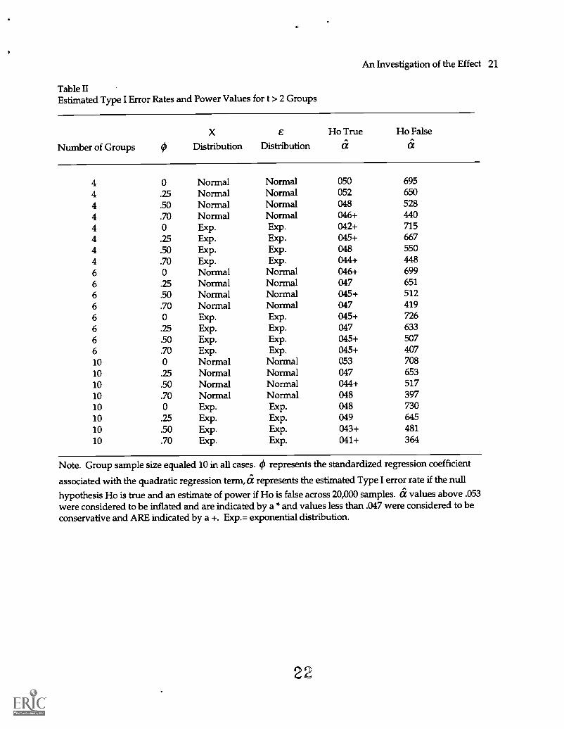
Table IIEstimated Type I Error Rates and Power Values for t > 2 Groups

Number of Groups 0

x e Ho True Ho False

Distribution Distribution a a

4 0 Normal Normal 050 695

4 .25 Normal Normal 052 650


4 .70 Normal Normal 046+ 440

4 0 Exp. Exp. 042+ 715

4 .25 Exp. Exp. 045+ 667

4 .50 Exp. Exp. 048 550

4 .70 Exp. Exp. 044+ 448

6 0 Normal Normal 046+ 699


6 .50 Normal Normal 045+ 512


6 0 Exp. Exp. 045+ 726

6 .25 Exp. Exp. 047 633

6 .50 Exp. Exp. 045+ 507

6 .70 Exp. Exp. 045+ 40710 0 Normal Normal 053 708


10 .50 Normal Normal 044+ 51710 .70 Normal Normal 048 39710 0 Exp. Exp. 048 730

10 .25 Exp. Exp. 049 645

10 .50 Exp. Exp. 043+ 481

10 .70 Exp. Exp. 041+ 364

Note. Group sample size equaled 10 in all cases. 0 represents the standardized regression coefficient

associated with the quadratic regression term, a represents the estimated Type I error rate if the null

hypothesis Ho is true and an estimate of power if Ho is false across 20,000 samples. a values above .053were considered to be inflated and are indicated by a * and values less than .047 were considered to beconservative and ARE indicated by a +. Exp.= exponential distribution.

22

AREA 1997

U.S. DEPARTMENT OF EDUCATIONOffice of Educational Research and Improvement (OERI)

Educational Resources information Center (ERIC)

REPRODUCTION RELEASE f ill 0 3

ERIC(Specific Document)

I. DOCUMENT IDENTIFICATION:

4ect aemAkeo2ZctxAN COVA-

Title: AA tic veskt.5_ act-i 0

J-etRAZSi1/4 of\ dicAuthor(s): V\ e I (Corporate Source:

U pm\;ers 6,-ti-Auri\II. REPRODUCTION RELEASE:

Publication Date:

R L1 (159

In order to disseminate as widely as possible timely and significant materials of interest to the educational community, documentsannounced in the monthly abstract journal of the ERIC system, Resources in Education (RIE). are usually made available to usersin microfiche. reproduced paper copy. and electronic/optical media. and sold through the ERIC Document Reproduction Service(EDRS) or other ERIC vendors. Credit is given to the source of each document, and, if reproduction release is granted, one ofthe following notices is affixed to the document.

If permissio granted to reproduce the identified document, please CHECK ONE of the following options and sign the release

below.

Check herePermittingmicrofiche(4"x 6" film),paper copy.electronic.and optical mediareproduction

Sample sticker to be affixed to document Sample sticker to be affixed to document

"PERMISSION TO REPRODUCE THISMATERIAL HAS BEEN GRANTED BY

TO THE EDUCATIONAL RESOURCESINFORMATION CENTER (ERIC):'

Laval 1

"PERMISSION TO REPRODUCE THISMATERIAL IN OTHER THAN PAPER

COPY HAS BEEN GRANTED BY

C

TO THE EDUCATIONAL RESOURCESINFORMATION CENTER (ERIC)."

Level 2

or here

Permittingreproductionin other thanpaper copy.

Sign Here, PleaseDocuments will be processed as indicated provided reproduction quality permits. If permission to reproduce is granted, but

neither box is checked. documents will be processed at Level 1.

"I hereby grant to the Educationalindicated above. Reproductionsystem contractors requires permissionService agencies to satisfy information

Resources Information Center (ERIC) nonexclusive permission to reproduce this document asfrom the ERIC microfiche or electronic/optical media by persons other than ERIC employees and its

from the copyright holder. Exception is made for non-profit reproduction by libraries and otherneeds of ducators in response to discrete inquiries."

Sigrlture: io, Position: ---

A5S° Ck6 -Nie5 S'preled tai \.\\

KKC OT-Ci1/4) 0Organization:

U g1/41: ilt:Itg 60 kAddress: S. C 0 \ - '"--iDr: Q UO40 \CI U g.

P G- plk 15 1)-(00

Telephone Number:( 4 \ 11 641S-1) I) r)1

Date:

14( /InOVER

UA

THE CATHOLIC UNIVERSITY OF AMERICADepartment of Education, O'Boyle Hall

Washington, DC 20064202 319-5120

February 21, 1997

Dear AERA Presenter,

Congratulations on being a presenter at AERA'. The ERIC Clearinghouse on Assessment andEvaluation invites you to contribute to the ERIC database by providing us with a printed copy ofyour presentation.

Abstracts of papers accepted by ERIC appear in Resources in Education (RIE) and are announcedto over 5,000 organizations. The inclusion of your work makes it readily available to otherresearchers, provides a permanent archive, and enhances the quality of RIE. Abstracts of yourcontribution will be accessible through the printed and electronic versions of RIE. The paper willbe available through the microfiche collections that are housed at libraries around the world andthrough the ERIC Document Reproduction Service.

We are gathering all the papers from the AERA Conference. We will route your paper to theappropriate clearinghouse. You will be notified if your paper meets ERIC's criteria for inclusionin RIE: contribution to education, timeliness, relevance, methodology, effectiveness ofpresentation, and reproduction quality. You can track our processing of your paper athttp://ericae2.educ.cua.edu.

Please sign the Reproduction Release Form on the back of this letter and include it with two copiesof your paper. The Release Form gives ERIC permission to make and distribute copies of yourpaper. It does not preclude you from publishing your work. You can drop off the copies of yourpaper and Reproduction Release Form at the ER C booth (523) or mail to our attention at theaddress below. Please feel free-to-copy the form fo fitture or additional submissions.

Mail to: AERA 1997/ERIC AcquisitionsThe Catholic University of AmericO'Boyle Hall, Room 210Washington, DC 20064

This year E C/AE is making a Searcha onference Program available on the AERA webpage (http: //ae net). Check _it out!'

ence M. Rudner, Ph.D.Director, ERIC/AE

'If you are an AERA chair or discussant, please save this form for future use.

ERIC] Clearinghouse on Assessment and Evaluation

Date post:	07-May-2018
Category:	Documents
Upload:	doanhanh
View:	215 times
Download:	1 times