DOCUMENT RESUME ED 286 930 TM 870 571 AUTHOR Plaut, David C.; And Others TITLE Experiments on Learning by Back Propagation. INSTITUTION Carnegie-Mellon Univ., Pittsburgh, Pa. Dept. of Computer Science. SPONS AGENCY Office of Naval Research, Washington, D.C. Personnel and Training Branch. REPORT NO CMU-CS-86-126 PUB DATE Jun 86 GRANT N00014-86-K-00167 NOTE 54p. PUB TYPE Reports - Research/Technical (143) EDRS PRICE MF01/PC03 Plus Postage., DESCRIPTORS *Artificial Intelligence; Cognitive Structures; .Computer Simulation; *Discrimination Learning; *Error Patterns; *Feedback; Learning Processes; *Learning Strategic- Learning Theories; Mathematical Models; Multidimensional Scaling; *Networks; Weighted Scores IDENTIFIERS *Connectionism; Iterative Methods ABSTRACT This paper describes further research on a learning procedure for layered networks of deterministic, neuron-like units, described by Rumelhart et al. The units, the way they are connected, the learning procedure, and the extension to iterative networks are presented. In one experiment, a network learns a set of filters, enabling it to discriminate format-like patterns in the presence of noise. The speed of learning strongly depends on the shape of the surface formed by the error measure in "weight space." Examples show the shape of the error surface for a typical task and illustrate how an acceleration method speeds up descent in weight space. The main drawback of the learning procedure is the way it scales as the size of the task and the network increases. Some preliminary scaling results show how the magnitude of the optimal weight changes depends on the fan-in of the units. A variation of the learning procedure that back-propagates desired state information rather than error gradients is developed and compared with the standard procedure. Finally, the relationship between these iterative networks and the "analog' networks described by Hopfield and Tank are discussed. (Author/LPG) *********************************************************************** Reproductions supplied by EDRS are the best that can be made from the original document. ***********************************************************************
Transcript
DOCUMENT RESUME
ED 286 930 TM 870 571
AUTHOR Plaut, David C.; And OthersTITLE Experiments on Learning by Back Propagation.INSTITUTION Carnegie-Mellon Univ., Pittsburgh, Pa. Dept. of
Computer Science.SPONS AGENCY Office of Naval Research, Washington, D.C. Personnel
and Training Branch.REPORT NO CMU-CS-86-126PUB DATE Jun 86GRANT N00014-86-K-00167NOTE 54p.PUB TYPE Reports - Research/Technical (143)
EDRS PRICE MF01/PC03 Plus Postage.,DESCRIPTORS *Artificial Intelligence; Cognitive Structures;
ABSTRACTThis paper describes further research on a learning
procedure for layered networks of deterministic, neuron-like units,described by Rumelhart et al. The units, the way they are connected,the learning procedure, and the extension to iterative networks arepresented. In one experiment, a network learns a set of filters,enabling it to discriminate format-like patterns in the presence ofnoise. The speed of learning strongly depends on the shape of thesurface formed by the error measure in "weight space." Examples showthe shape of the error surface for a typical task and illustrate howan acceleration method speeds up descent in weight space. The maindrawback of the learning procedure is the way it scales as the sizeof the task and the network increases. Some preliminary scalingresults show how the magnitude of the optimal weight changes dependson the fan-in of the units. A variation of the learning procedurethat back-propagates desired state information rather than errorgradients is developed and compared with the standard procedure.Finally, the relationship between these iterative networks and the"analog' networks described by Hopfield and Tank are discussed.(Author/LPG)
***********************************************************************Reproductions supplied by EDRS are the best that can be made
from the original document.***********************************************************************
19 ABSTRACT (Continue on niverse if necessary and identify by block number)
OVER
20. DISTRIBUTION/AVAILABILITY OF ABSTRACT
0 UNCLASSIFIED/UNLIMITED M SAME AS RPT. 0 DTIC USERS
-----21. ABSTRACT SECURITY CLASSIFICATION
Unclassified22a. NAME OF REPON5I3LE INDIVIDUALDr. Harold Hawkins
22b. TELEPHONE (Include Area Code)202-696-4323
22c. OFFICE SYMZICI.I.
1142PT
Previous editions are obsolete. SECURITY CLASSIFICATION OF THIS PAGE
UNCLASSIFIED
Abstract
Rumelhart, Hinton and Williams [Rumelhart 86] describe a learning procedure for layered networks of
deterministic, neuion-like units. This paper describes further research on the learning procedure. We start by
describing the units, the way they are connected, the learning procedure, and the extension to iterative nets. We then
give an example in which a network learns a set of filters that enabla it to discriminate formant -like patterns in the
presence of noise.
The speed of learning is strongly dependent on the shape of the surface formed by the error measure in "weight
space." We give examples of the shape of the error surface for a typical task and illustrate how an acceleration
method speeds up descent in weight space.
The main drawback of the learning procedure is the way it scales as the size of the task and the network increases.
We give some preliminary results on scaling and show how the magnitude of the optimal weight changes depends
on the fan-in of the units. Additional results illustrate the effects on learning speed of the amount of interaction
between the weights. .
A variation of the learning procedure that back-propagates desired state information rather than error gradients is
developed and compared with the standard procedure.
Finally, we discuss the relationship between our iterative networks and the "analog" networks described by
Hopfiell and Tank [Hopfield 85]. The learning procedure can discover appropriate weights in their kind of network,
as well as determine an optimal schedule for varying the nonlinearity of the units during a search.
4
Table of Contents1. Introduction 1
1.1. The Units 1
1.2., Layered Feed-forward Nets 213. The Learning Procedure 21.4. The Extension to Iterative Nets 4
2. Learning to Discriminate Noisy Signals 63. Characteristics of Weight Space 104. How the Learning Time Scales 19
4.1. Experiments 194.2. Unit Splitting 2043. Varying Epsilon with Fan -In 21
5. Reducing the Interactions between the Weights 225.1. Experiments 225.2. Very fast learning with no generalization 23
6. Back Propagating Desired States 236.1. General Approach 246.2. Details 2563. General Performance 256.4. Scaling Performance 266.5. Conclusions on Back Propagating Desired States 27
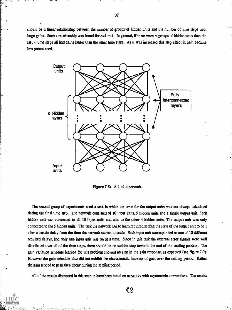
7. Gain Variation in Iterative Nets 277.1. Introduction Z/7.2. Implementation of Gain Variation 3073. Experimeital Results 31
Cv
1
1. IntroductionRumelhart, Hinton and Williams [Rumelhart 86] describe a learning procedure for layered networks of
deterministic, neuron-like units. The procedure repeatedly adjusts the weights in the network so as to minimize a
measure of the difference between the actual output vector of the net and the desired output vector given the current
input vector. This report describes further research on the learning procedure.
We start by describing the units, the way they are connected, the learning procedure, and the extension to iterative
nets. We then give an example in which a network learns a set of filters that enable it to discriminate formant-like
patterns in the presence of noise. The example shows how the learning procedure discovers weights that turn units
in intermediate layers into an "ecology" of useful feature detectors each of which complements the other detectors.
The speed of learning is strongly dependent on the shape of the surface formed by the error measure in "weight
space." This space has one dimension for each weight in the network and one additional dimension (height) that
represents the overall error in the network's performance for any given set of weights. For many tasks, the error
surface contains ravines that cause problems for simple gradient descent procedures. We give examples of the shape
of the error surface for a typical task and illustrate the advantages of using an acceleration method to speed up
progress down the ravine without causing divergent "sloshing" across the ravine.
The main drawback of the learning procedure is the way it scales as the size of the task and the network increases.
We give some preliminary results on scaling and show how the magnitude of the optimal weight changes depends
on the fan-in of the units. Additional results illustrate the effects on learning speed of the amount of interaction
between the weights.
A variation of the learning procedure that back-propagates desired state information rather than error gradients.is
developed and compared with the standard procedure.
Finally, we discuss the relationship between our iterative networks and the "analog" networks described by
Hopfield and Tank [Hopfield 85]. The learning procedure can be used to discover appropriate weights in their kind
of network. It can also be used to determine an optimal schedule for varying the nonlinearity of the units during a
search.
1.1. The Units
The total input, xj, to unit j is a linear function of the e iiputs of the units, i, that are connected to j and of the
weights, wii, on these connections.
Xj rs I yiwii (1)i
A unit has a real-valued output, yj, that is a non-linear function of its total input.
yi -1
(2)1 + ix'
It is not necessary to use exactly the functions given by Eqs. 1 and 2. Any input-output function that has a bounded
2
derivative will do. However, the use of a linear function for combining the inputs to a unit before applying the
nonlinearity greatly simplifies the learning procedure.
1.2. Layered Feed-forward Nets
The simplest form of the learning procedure is for layered networks that have a layer of input units at the bottom,
any number of intermediate layers, and a layer of output units at the top. Connections within a layer or from higher
to lower layers are forbidden. The only connections allowed are ones from lower layers to higher layers, but the
layers do not need to be adjacent; connections can skip layers.
An input vector is presented to the network by setting the states of the input units. Then the states of the units in
each layer are determined by applying Eqs. 1 and 2 to the connections coming from lower layers. All units within a
layer have their states set in parallel, but different layers have their states set sequentially, starting at the bottom and
working upwards until the states of the output units are determined.
13. The Learning Procedure
The aim of the learning procedure is to find a set of weights which ensures that for each input vector the output
vector produced by the network is the same as (or sufficiently close to) the desired output vector. If there is a fixed,
fmite set of input-output cases, the total error in the performance of the network with a particular set of weights can
be computed by comparing the actual and desired output vectors for every case. The error, E, is defined by
v.. v.E' Il..a.4(Yi.cfild2c j
where 0 is an index over cases (input-output pairs), j is an index over output units, y is the actual state of an output
unit, and d is its desired state. To minimize E by gradient descent it is necessary to compute the partial derivative
of E with respect to each weight in the network. This is simply the sum of the partial derivatives for each of the
input-output cases. For a given case, the partial derivatives of the error with respect to each weight are computed in
two passes. We have already described the forward pass in which the units in each layer have their states
determined by the input they receive from units in lower layers using Eqs. 1 and 2. The backward pass that
propagates derivatives from the top layer back to the bottom one is more complicated.
(3)
aEThe backward pass starts by computing for each of the output units. Differentiating Eq. 3 for a particular case,
ayc, and suppressing the index c gives
aE--a. yd,yI "
We can then apply the chain rule to computeaEat '
1
aE aE .dY;
ail dx/
dy,Differentiating Eq. 2 to get the value of .: gives
"i
3
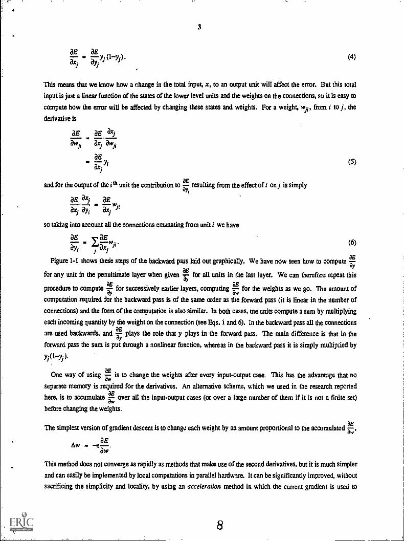
aE aEaz Kyj(iYj).
1 -'1(4)
This means that we know how a change in the total input, x, to an output unit will affect the error. But this total
input is just a linear function of the states of the lower level units and the weights on the connections, so it is easy to
compute how the error will be affected by changing these states and weights. For a weight, wii, from i to j, the
derivative is
aE aE ax;xawf..a aw..
t 1 ft
aE57
1Yi
and for the output of the ith unit the contribution to P-E.i
resulting from the effect of i on j is simplyar
(5)
aE .ax; aEax; ayi ax; fi
so taking into account all the connections emanating from unit i we have
aE v aE(6)a
ayi taxi J`Figure 1-1 shows theie steps of the backward pass laid out graphically. We have now seen how to compute Ply.
DEfor any unit in the penultimate layer when given -- fix all units in the last layer. We can therefore repeat this
DE DEprocedure to compute Ty for successively earlier layers, computing . for the weights as we go. The amount of
computation required for the backward pass is of the same order as the forward pass (it is linear in the number of
connections) and the form of the computation is also similar. In both cases, me units compute a sum by multiplying
each incoming quantity by the weight on the connection (see Eqs. 1 and 6). In the backward pass all the connections
are used backwards, and I plays the role that y plays in the forward pass. The main difference is that in thear
forward pass the sum is put through a nonlinear function, whereas in the backward pass it is simply multiplied by
Yi(1Yi).
aEOne way of using is to change the weights after every input-output case. This has the advantage that no
aw
separate memory is required for the derivatives. An alternative scheme, which we used in the research reported
here, is to accumulateDE
over all the input-output cases (or over a large number of them if it is not a finite set)aw
before changing the weights.
DEThe simplest version of gradient descent is to change each weight by an amount proportional to the accumulated y,,,
ulw.w e aE--.aw
This method does not converge as rapidly as methods that make use of the second derivatives, but it is much simpler
and can easily be implemented by local computations in parallel hardware. It can be significantly improved, without
sacrificing the simplicity and locality, by using an acceleration method in which the current gradient is used to
Output layer 0aeaxi - aeayi . yi (1 - yi )
44 a E/awil - aeaxi . yi
411
4
aE/ayi . yi - cij
aeayi - II aeaxi . wii
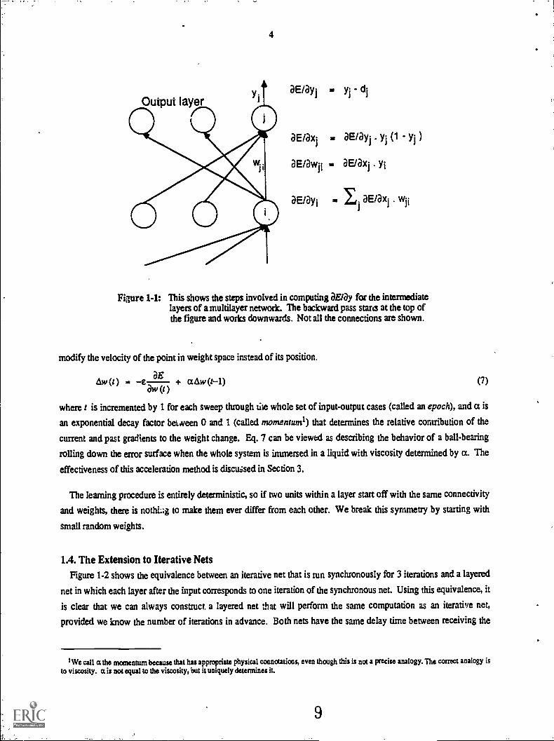
Figure 1-1: This shows the steps involved in computing aE/ay for the intermediatelayers of a multilayer network. The backward pass starts at the top ofthe figure and works downwards. Not all the connections are shown.
modify the velocity of the point in weight space instead of its position.
ow (t) - awaE + aAw(t-1) (7)
where t is incremented by 1 for each sweep through tile whole set of input-output cases (called an epoch), and a is
an exponential decay factor between 0 and 1 (called momentwnl) that determines the relative contribution of the
current and past gradients to the weight change. Eq. 7 can be viewed as describing the behavior of a ball-bearing
rolling down the error surface when the whole system is immersed in a liquid with viscosity determined by a. The
effectiveness of this acceleration method is discussed in Section 3.
The learning procedure is entirely deterministic, so if two units within a layer start off with the same connectivity
and weights, there is nothi4 to make them ever differ from each other. We break this symmetry by starting with
small random weights.
1.4. The Extension to Iterative NetsFigure 1-2 shows the equivalence between an iterative net that is run synchronously for 3 iterations and a layered
net in which each layer after the input corresponds to one iteration of the synchronous net. Using this equivalence, it
is clear that we can always construct a layered net that will perform the same computation as an iterative net,
provided we know the number of iterations in advance. Both nets have the same delay time between receiving the
IWe call a the momentum because that hu appropriate physical connotations, even though this is not a precise analogy. The correct analogy isto viscosity. a is not equal to the viscosity, but it uniquely determines it.
input and giving the output.
S
A set ofcorresponding
weights
W2' Wt
CC:=01
W3
A simple iterative ;let thatis run for thrse iterations An equivalent layered net
Figure 1.2: An iterative net and the equivalent layered net.
Since we have a learning procedure for layered nets, we could learn iterative computations by first constructing
the equivalent layered net, then doing the learning, then converting back to the iterative net. Or we could avoid the
construction by simply mapping the learning procedure itself into the form appropriate for the iterative net. Two
complications arise in performing this conversion:
1. In a layered net the outputs of the units in th: intermediate layers during the forward pass are requiredfor performing the backward pass (see Eqs. 4 and 5). So in an iterative net it is necessary to store theoutput states of each unit that are temporally intermediate between the initial and final states.
2. For a layered net to be equivalent to .ut iterative net, corresponding weights between different layersmust have the same value, as in figure 1-2. There is no guarantee that the basic learning procedure forlayered nets will preserve this property. However, we can easily modify it by averaging aE/aw for allthe weights in each set of corresponding weights, and then changing each weight by ad amountproportional to this average gradient. This is equivalent to taking the weight-change vector producedby the basic learning procedure and then projecting it onto the subspace of layered nets that areequivalent to iterative ones.
With these two provisos, the learning procedure can be applied directly to iterative nets and can be used to learn
sequential structures. Several examples are given in [Rumelhart 86]. We return to iterative nets at the end of this
paper and show how the learning procedure can be further modified to allow it to learn how to vary the nonlinearity
in Eq. 2 as the network settles.
10
6
2. Learning to Discriminate Noisy SignalsRumelhart, Hinton, and Williams plume lhart 86] illustrate the performance of the learning procedure on many
different, simple tasks. We give a further example here which demonstrates that the procedure can construct sets of
filters that are good at discriminating between rather similar signals in the presence of a lot of noise. We used an
artificial task (suggested by Alex Waibel) which was ;ntended to resemble a task that arises in speech recognition.
We are currently working on extending this approach to real speech data.
The input is a synthetic spectrogram that represents the energy in six different frequency bands at nine different
times. Figure 2-1 shows examples of spectrograms with no random variation in the level of the signal or the
background, and figure 2-2 shows examples with added noise. The problem is to decide whether the signal is
simply a horizontal track or whether it rises at the beginning. There is variation in both the frequency and onset time
of the signal.
It is relatively easy to decide on the frequency of the horizontal part of the track, but it is much harder to
distinguish the "risers" from the "non-risers" because the noise in the signal and background obscures the rise. To
make the distinction accurately, the network needs to develop a set of filters that are carefully tuned to the critical
differlices. The filters must cove the range of possible frequencies and onset times, and when several different
filters fit quite well, their outputs must be correctly weighted to give the right answer.
We used a network with three layers as shown in figure 2-3. Initially we tried training the network by repeatedly
sweeping through a fixed set of 1000 examples, but the network learned to use the structure of the noise to help it
discriminate the difficult cases, and so it did not generalize well when tested on new examples in which the noise
was different. We therefore decided to generate a new example every time so that, in the long run, there were no
spurious correlations between the noise and the signal. Because the network lacks a strong a priori model of the
nature of the task, it has no way of telling the difference between a spurious correlation caused by using too small a
sample and a systematic 'correlation that reflects tht: structure of the task.
Examples were generated by the following procedure:
1. Decide to generate. a riser or a non-riser with equal probability.
2. If it is a non-riser pick one of the six frequencies at random. If it is a riser pick one of the four highestfrequencies at random (the final frequency of a riser must be one of these four because it must risethrough two frequency bands at the beginning).
3. Pick one of 5 possible onset times at random.
4. Give each of the input units a value of 0.4 if it is part of the signal and a value of 0.1 if it is part ol thebackground. We now have a noise-free spectrogram of the kind shown in figure 2-1.
5. Add independent gaussian noise with mean 0 and standard deviation 0.15 to each unit that is part ofthe signal. Add independent gaussian noise with mean 0 and standard deviation 0.1 to the background.If any unit now has a negative activity level, set its level to 0.
The weights were modified after each block of 25 examples. For each weight, the values ofaE
were summed foraw
all 25 cases and the weight increment after block t was given by Eq. 7. For the first 25 examples we used e=0.005
and a=0.5. After this the weights changed rather slowly and the values were raised to e=0.07 and a=0.99. We have
found that it is generally helpful to use more conservative values at the beginning because the gradients are initially
A layer of 24 hiddenunits each of whichis connected to all54 input units and toboth output units
A layer of 54 inputunits whose activitylevels encode theenergy in six frequencybands for nine timeintervals.
Figure 2-3: The net used for discriminating patterns like those in figure 2-2.
very steep and the weights tend to overshoot. Once the weights have settled down, they are near the bottom of a
ravine in weight space, and high values of a are required to speed progress along the ravine and to damp out
oscillations across the ravine. We discuss the validity of interpreting characteristics of weight space in terms of
structures such as ravines in Section 3.
In addition to the weight changes defined by Eq. 7, we also incremented each weight by hw each time it was
changed, where h is a coefficient that was set at 0.001% fo; this simulation. This gives the weights a tendency to
decay towards zero, eliminating weights that are not doing any useful work. The It w term ensures that weights for
whichaE
is near zero will keep shrinking in magnitude. Indeed, at equilibrium the magnitude of a weight will healv
proportional to r- and so it will indicate how important the weight is for performing the task correctly. This makes
it much easier to understand the feature detectors produced by the learning. One way to view the term hw is as the
derivative of Ihw2, so we can view the learning procedure as a compromise between minimizing E and
minimizing the sum of the squares of the weights.
Figure 2-4 shows the activity levels of the units in all three layers for a number of examples chosen at random
after the network has learned. Notice that the network is normally confident about whether the example is a riser or
a non-riser, but that in difficult cases it tends to hedge its bets. This would provide more useful information to a
higher level process than a simple forced choice. Notice also that for each example, most of the units in the middle
layer are firmly off.
13
112 - su -ss . Jal '- , mssa .. a a Elm ,, 14 119, III - ,
. . . . Ag . ra.a 4 . ' n c a a - , capR estate II I Ca 2
. :7 ' . a ` -, 11( s.e g ... . a .,_ a II. r Go :la R a li a a - a>
152.m .....el el . - a . II a m * Olg 63 as RI a. , a go. _4. .. . , a . . a I 3 Ifi RIO a -"a 1 la . a kij I I - a
s
SS a Rees ma a .. . al ..k 4 mi
ga cam 12 a®® a
(., ill MI igi IN El Iii a a4 . gli a - a . Itl gii al N' N
t. . a ...
a ft . , , a a Eil PI la g -,.. a
arc
. 4 : .. .. ,
n
a
: .5, i' ta
lit
n 2 cl
t .. 0 l
. EI . gti 0 a . as ,CI CA 6
s112, . . Es, ill Ed RI F 2 . V. . El la Figha ED la ® i
Sit a fa a m a:, %
. I I CS ill Fria II . a IL aso a s . i m a a . . a ago g. .iiago II alb.aa
g2 Ilk 12 C a vIR . RIM 11111 NM
. a Iii IR a a raII 4 . Si 111 ...
1. ,..-
r Ea IIII a - , a * , 0 a ill iff a a . U n in ai M' !I
ID a . Mt
,N
- -
rd. -1.1 r3 Elrao te m
0.
aaffiara a.
e's a a 's ' PEE Nal: IL aa./ISa. 55a la
vea , .. am
It Ns-
a awnNa N N IIII. gl . .. . . -
a Al 0 a el In 0 0 a ENm . \ 'a
e - 0
a 0 ID n t 1 II111.kms
al I a
I
ellren o n
a
a tia . a
lal 1
arh a ii. pii ...N.... . ala
E:11:313 me MI IS El . in 0 -11 ELMEA
Irv.
111 - IS Ea
I li Et. .
a
a a
da a a 13.1
a, a
a
=
IQ
3
=
2.12====================32
211=.... = _ = = =
:TM
=
==t = = XS 2111=2'"... = -
= =
= = -... = --
Jig 31=
- -
=
-----
VEIL '".".. 3
- - 2 =
==t =2 St = =
==.1= ==as = ==== =
= === = = = XX =
== = =
= =
= 3.= = =
,
=
=
Figure 24: Some of the filters learned by the middle layer. Each weight is represented bya square whose size is proportional to the magnitude of the weight and whosecolor represents the sign of the weight (white for positive, black for negative).
15
11
The network was trained for 10,000 blocks of 25 examples each. After this amount of experience the weights are
very stable and the performance of the network has ceased to improve. If we force the network to make a discrete
decision by interpreting the more active of the two output units as its response, it give the "correct" response 97.8%
of the time. This is better than a person can do Using elaborate reasoning, and it is probably very close to the
optimal possible performance. No system could get 100% correct because the very same data can be generated by
adding noise to two different underlying signals, and hence it is not possible to recover the underlying signal from
the data with certainty. The best that can be done is to decide which category of signal is most likely to have
produced the data and this will sometimes not be the category from which the data was actually derived. For
example, with the signal and noise levels used in this example, there is a probability of about 1.2% that the two
crucial input units that form the rising part of a riser will have a smaller combined activity level than the two units
that would form part of a non-riser with the same onset time and same final frequency. This is only one of several
possible errors.
Figure 2-5 shows the filters that were learned in the middle layer. The ones that have positive weights to the
"riser" output unit have been arranged at the top of the figure. Their weights are mainly concentrated on the part of
the input that contains the critical information, and between them they cover all the possible frequencies and onset
times. Notice that each filter covers several different cases and that each case is covered by several different filters.
The set of filters form an "ecology" in which eagh nne fills a niche that is left by the others. Using analytical
methods it would be very hard to design a set of filters with this property, even if the precise characteristics of the
process that generated the signals were explicitly given. The difficulty arises because the definition of a good set of
filters is one for which there exists a set of or put weights that allows the correct decision to be made as often as
possible. The input weights of the filters cannot be designed without considering the output weights, and an
individual filter cannot be designed without considering all the other filters. This means that the optimal value of
each weight depends on the value of every other weight. The learning procedure can be viewed as a numerical
method for solving this analytically intractable design problem. Current analytical investigations of optimal
filters [Torre 86) are very helpful in providing unde:standing of why some filters are the way they are, but they shed
little light on how biological systems could arrive at these designs.
3. Characteristics of Weight SpaceAs mentioned in the Introduction, a useful way to interpret the operation of the learning procedure is in terms of
movement down an error surface in multi-dimensional weight space. For a network with only two connections, the
characteristics of the error surface for a particular task are relatively easy to imagine by analogy with actual surfaces
which curve through three-dimensional physical space. The error surface can be described as being comprised of
hills, valleys, ravines, ridges, plateaus, saddle points, etc. In the learning procedure, the effects of the weight-change
step (e) and momentum (a) parameters have natural interpretations in terms of physical movement among such
formations. Unfortunately, for more useful networks with hundreds or thousands of connections it is not clear that
these simple intuitions about the characteristics of weight space are valid guides to determining the parameters of the
learning procedure.
One way to depict some of the structure of a high-dimensional weight space is to plot the error curies (i.e.
16
12
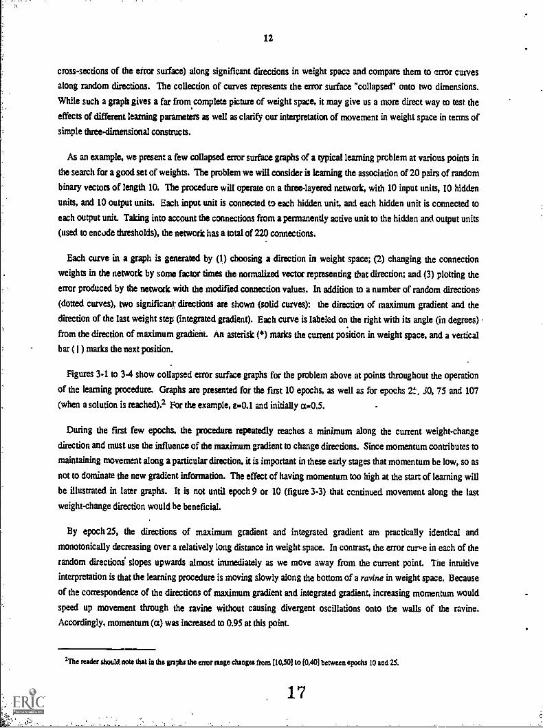
cross-sections of the error surface) along significant directions in weight space and compare them to error curves
along random directions. The collection of curves represents the error surface "collapsed" onto two dimensions.
While such a graph gives a far from complete picture of weight space, it may give us a more direct way to test the
effects of different learning parameters as well as clarify our interpretation of movement in weight space in terms of
simple three-dimensional constructs.
As an example, we present a few collapsed error surface graphs of a typical learning problem at various points in
the search for a good set of weights. The problem we will consider is learning the association of 20 pairs of random
binary vectors of length 10. The procedure will operate on a three-layered network, with 10 input units, 10 hidden
units, and 10 output units. Each input unit is connected to each hidden unit, and each hidden unit is connected to
each output unit. Taking into account the connections from a permanently active unit to the hidden and output units
(used to encode thresholds), the network has a total of 220 connections.
Each curve in a graph is generated by (1) choosing a direction in weight space; (2) changing the connection
weights in the network by some factor times the normalized vector representing that direction; and (3) plotting the
=or produced by the network with the modified connection values. In addition to a number of random directions.
(dotted curves), two significant directions are shown (solid curves): the direction of maximum gradient and the
direction of the last weight step (integrated gradient). Each curve is labeled on the right with its angle (in degrees)
from the direction of maximum gradient. An asterisk (*) marks the current position in weight space, and a vertical
bar ( I ) marks the next position.
Figures 3-1 to 3-4 show collapsed error surface graphs for the problem above at points throughout the operation
of the learning procedure. Graphs are presented for the first 10 epochs, as well as for epochs 2t, .i0, 75 and 107
(when a solution is reached)? For the example, e.0.1 and initially co.0.5.
During the first few epochs, the procedure repeatedly reaches a minimum along the current weight-change
direction and must use the influence of the maximum gradient to change directions. Since momentum contributes to
maintaining movement along a particular direction, it is important in these early stages that momentum be low, so as
not to dominate the new gradient information. The effect of having momentum too high at the start of learning will
be illustrated in later graphs. It is not until epoch 9 or 10 (figure 3-3) that continued movement along the last
weight-change direction would be beneficial.
By epoch 25, the directions of maximum gradient and integrated gradient are practically identical and
monotonically decreasing over a relatively long distance in weight space. In contrast, the error cum in each of the
random directioni slopes upwards almost immediately as we move away from the current point. Tne intuitive
interpretation is that the learning procedure is moving slowly along the bottom of a ravine in weight space. Because
of the correspondence of the directions of maximum gradient and integrated gradient, increasing momentum would
speed up movement through the ravine without causing divergent oscillations onto the walls of the ravine.
Accordingly, momentum (a) was increased to 0.95 at this point.
21lte reader should. note that in the graphs the error range changes from (10,501 to (0,401 between epochs 10 and 25.
17
'DU
10
5-1
L0(
i-
ll
r-
4.)
04-1
1A
-5i
weight change factor
epoch 1
Cj
\
0
78Er?8b
I c-9 .
weight chanqe factor
epoch 3
0
2891
8396
13
50
10
50
10
s',...... \."..,......A
////.."./
-5 .
cJweight change factor
epoch 2
C I CIiweiqht chary factor
epoch 4
Figure 3.1: Collapsed error surfaces for epochs 1 to 4.
18
21
0
50
10
5W
..0
//. ' ../ / ./
/
//''....*
1i
-5wei ght change factor
040
959289
14
50
r
0L.
IM
n
10
\N\ \\ \\\\\\
/ ....---'
/. ,
..-. -
..'... 1 //\ //::.-.: : : ; 1 ...t.....:.'':
a-J
weight t change factor
epoch 5 epoch 6
"-....--'\........
\ \ / . ..N. ,. / .44.
\,....\/ .:;,:-:".
"... //..'....i-
JWe i ght change factor
epoch 7
09235
BB
50
10
5
28979535
/
-5weight change factor
epoch 8
Figure i.2: Collapsed error surfaces for epochs 5 to 8.
5
0
50
L0LLat
.--to
4.)04.)
10
40
L0L
di
rto
4.)04-)
ei
1-5weight change factor
5
epoch
N7:77....Ak--,__
..
. : '. .... .7--- ; ; ; : ' :
. ... 7 .. . + I, : . L:
-....-"-....--m....mm
c1-5 ...I
weight change factor
g89
0
949+93
e2.
15
50
L0Li'
Vii
I--ID4.)04.)
10I c-5
weight change factor.I
epoch 10
401
L0fal
M4)04)
....:-....
-................"-.......a.j,.....--...,
t ' .. :
:. : ....._...."
el......
1
weight change factor
epoch 25 epoch 50
Figure 3.3: Collapsed error surfaces for epochs 9 to 50
20
cJ
51
40
0L.
iq
0
A
;
9282
X91
-5ei ght
epoch 75
change factor5
59
16
40
009
-5 5weight change factor
epoch 107 (solmtion)
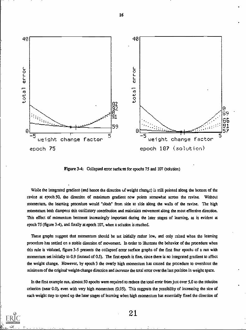
Figure 3.4: Collapsed error surfwes for epochs 75 and 107 (solution)
While the integrated gradient (and hence the direction of weight change) is still pointed along the bottom of the
ravine at epoch 50, the direction of maximum gradient now points somewhat across the ravine. Without
momentum, the learning procedure would "slosh" from side to side along the walls of the ravine. The high
momentum both dampens this oscillatory contribution and maintains movement along the most effective direction.
This effect of momentum becomes increasingly important during the later stages of learning, as is evident at
epoch 75 (figure 3-4), and finally at epoch 107, when a solution is reached.
These graphs suggest that momentum should be set initially rather low, and only raised when the learning
procedure has settled on a stable direction of movement. In order to illustrate the behavior of the procedure when
this rule is violated, figure 3-5 presents the collapsed' error surface graphs of the first four epochs of a run with
momentum set initially to 0.9 (instead of 0.5). The first epoch is fine, since there is no integrated gradient to affect
the weight change. However, by epoch 3 the overly high momentum has caused the procedure to overshoot the
minimum of the original' weight-change direction and increase the total error over the last position in weight space.
In the first example run, almost 50 epochs were required to reduce the total error from just over 5.0 to the solution
criterion (near 0.0), even with very high momentum (0.95). This suggests the possibility of increasing the size of
each weight step to speed up the later stages of learning when high momentum has essentially fixed the direction of
21
SG9157
0,.b kJ
0LIII
1"..*
M4)04-1
10
60
L
LL0
1.--M.004.)
10
.....
-5weight change factor
5
9.39284
17
L
LLIlj
rM.00-0
10
N._-.,-, \\ \ ,
..... . .
..
%
\`.%
\go st
/ //// ::, / . .,..4.: : : " . .:;/'
1
5-5weight change factor
epoch 1 epoch.2
::::::::
...
-5weight change factor
5
0
106
89se91
60
L0LLgi
IM.004)
10
\
5-5weight change factor
epoch 3 epoch 4
Figure 3-5: Collapsed error surfaces for the first four epochsof a run beginning with high momentum (a=0.9)
22
16
0
905
88
0
95
91
84al
1;0
LL
4.)
10
60
LlJ
L
13
1.)
4-)
10
13
-5we i ght change factor
epoch 1
5
90
8'3
/900/: :
, ; !). 90.....0*- 4+
L0LL
r-ip
4-)0
4-)
10
60
L0LLQU
0
" : : : ... " ......... :::::
ti
//
weight change factor
epoch'2
Ci
,i\\\....
/
42
.4//
N-::,. .// 90: ..... .. *-...,,,.. :::-: RI
......_,3 r
-5 I cin
J..., -5
I c
weight change factor weight change factor
epoch 3 epoch 4
Figure 3.6: Collapsed error surfaces for the first four epochs ofa run beginning with a large weight step (e=0.5).
23
19
weight change. In fact, increasing e does significantly reduce the number of epochs to solution, as long as the
weight step is not so large that the procedure drastically changes direction. However, because a number of changes
of direction ar4 required in the early stages of learning, the weight step must not be too large initially. Figure 3-6
illustrates the divergent behavior that results at the beginning of a run with e set to 0.5 (instead of 0.1). The first step
drastically overshoots the minimum along the direction of maximum gradient. Successive steps, though smaller, are
still are too large to produce coherent movement.
4. How the Learning Time ScalesSmall-scale simulations can only provide insight into the behavior of the learning procedure in larger networks if
there is information about how the learning time scales. Procedures that are very fast for small examples but scale
exponentially are of little interest if the goal is to understand learning in networks with thousands or millions of
units. There are many different variables that car, be scaled:
1. The number of units used for the input and output vectors and the fraction of them that are active inany one case.
2. The number of hidden layers.
3. The number of units in each hidden layer.
4. The fan-in and fan-out of the hidden units.
5. The number of different input-output pairs that must be learned, or the complexity of the mappingfrom input to output.
Much research remains to be done on the effects of most of these variables This section only addresses the question
of what happens to the learning time when the number of hidden units or layers is increased but the task and the
input-output encoding remain constant. If there is a fixed number of layers, we would like the learning to go faster
if the network has more hidden units per layer.
4.1. Experiments
Unfortunately, two initial experiments showed that increasing the number of hidden units or hidden layers slowed
down the learning? In the first, two networks were compared on the identical task: learning the associations of 20
pairs of random binary vectors of length 10. Each network consisted of three layers, with 10 input units and 10
output units. The first (called a 10-10-10 network) had 10 hidden units receiving input from all 10 input units and
projecting to all 10 output units; the second (called a 10-100-10 network) had 100 hidden units fully interconnected
to both input and output units. Twenty runs of each network on the task were carried out, with e.0.1 and a...0.8.
The results of this first experiment made it clear that the learning procedure in its current form does not scale well
with the addition of hidden units: the 10-10-10 network took an average of 212 epochs to reach solution, while the
10-100-10 network took an average of 531 epochs.4
3We measure learning time by the number of sweeps through the set of cases that are required to reach criterion. So the extra time requiredtosimulate a larger network on a serial machine is not counted.
4111e reader will note that the example run presented in Section 3 on the apparently identical task as described here took a network with 10hidden units only 107 epochs to solve. The difference is due to the use of a different set of 20 random binary vector pairs in the task.
24
20
The second experiment involved adding additional layers of hidden units to a network and seeing how the
different networks compared on the same task. The task was similar to the one above, but only 10 pairs of vectors
. were used Each network had 10 input units fully interconnected to units in the first hidden layer. Each hidden layer
had 10 units and was fully interconnected to the following one, with the last connected to the 10 output units.
Networks with one two and four layers of hidden units were used Twenty runs of each network were carried out,
with c -0.1 and a.0.8.
The results of the second experiment were consistent with those of the first: the network with a single hidden
layer solved the task in an average of 100 epochs; with two hidden layers it took 160 epochs on average, and with
four hidden layers it took an average of 373 epochs to solve the task.
4.2. Unit Splitting
There is method of introducing more hidden units which has no effect on the performance of the network.
Each hidden unit in the old network is replaced by n identical hidden units in the new network. The input weights
of the new units are exactly the same as for the old unit, so the activity level of each new unit is exactly the same as
for the old one in all circumstances. The output weights of the new units are each ,1; of the output weights of the old
unit, and so.their combined effect on any other unit is exactly the same as the effect of the single old unit. Figure
4-1 illustrates this invariant unit-splitting operation. To ensure that the old and new networks remain equivalent
even after learning, it is necessary for the outgoing weights of the new units to change by n times as much as the
outgoing weights of the old unit. So we must use a different value of c for the incoming and outgoing weights, and
the c for a connection emanating from a hidden unit must be inversely proportional to the fan-in of the unit receiving
the connection.
Figure 4.1: These two networks have identical input-output functions. The input-outputbehavior is invariant under the operation of splitting intermediate nodes,
provided the outgoing weights are also decreased by the same factor.
25
21
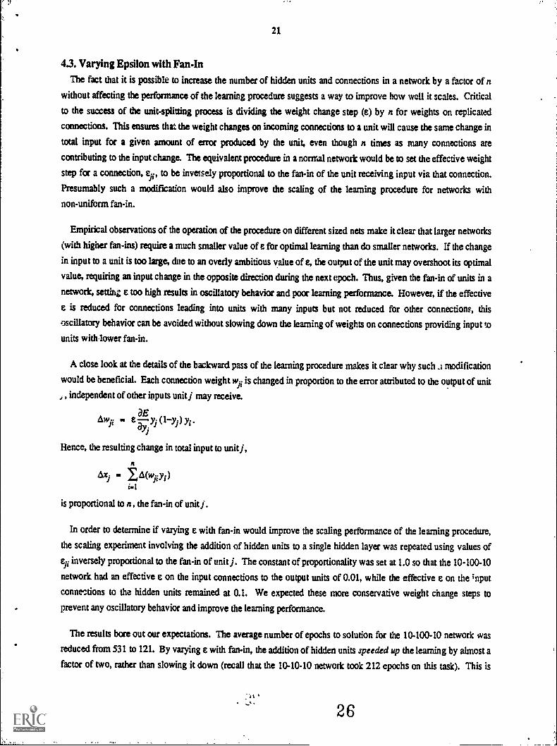
4.3. Varying Epsilon with Fan-In
The fact that it is possible to increase the number of hidden units and connections in a network by a factor ofn
without affecting the performance of the learning procedure suggests a way to improve how well it scales. Critical
to the success of the unit-splitting process is dividing the weight change step (e) by n for weights on replicated
connections. This ensures that the weight changes on incoming connections to a unit will cause the same change in
total input for a given amount of error produced by the unit, even though n times as many connections are
contributing to the input change. The equivalent procedure in a normal network would be to set the effective weight
step for a connection, e1, to be inversely proportional to the fan-in of the unit receiving input via that connection.
Presumably such a modification would also improve the scaling of the learning procedure for networks with
non-uniform fan-in.
Empirical observations of the operation of the procedure on different sized nets make it clear that larger networks
(with higher fan-ins) require a much smaller value of e for optimal learning than do smaller networks. If the change
in input to a unit is too large, due to an overly ambitious value of e, the output of the unit may overshoot its optimal
value, requiring an input change in the opposite direction during the next epoch. Thus, given the fan-in of units in a
network, setting e too high results in oscillatory behavior and poor learning performance. However, if the effective
e is reduced for connections leading into units with many inputs but not reduced for other connections, this
oscillatory behavior can be avoided without slowing down the learning of weights on connections providing input to
units with lower fan-in.
A close look at the details of the backward pass of the learning procedure makes it clear why such .; modification
would be beneficial. Each connection weight wji is changed in proportion to the error attributed to the output of unit
, independent of other inputs unit j may receive.
Aw- = eaE1
y.(1y.) yi.Av. 1-J1
Hence, the resulting change in total input to unit j,
1 It= A(w..y.)
is proportional to n, the fan-in of unit j.
In order to determine if varying e with fan-in would improve the scaling performance of the learning procedure,
the scaling experiment involving the addition of hidden units to a single hidden layer was repeated using values of
e- inversely proportional to the fan-in of unit j. The constant of proportionality was set at 1.0 so that the 10-100-10
network had an effective e on the input connections to the output units of 0.01, while the effective e on the ;nput
connections to the hidden units remained at 0.1. We expected these more conservative weight change steps to
prevent any oscillatory behavior and improve the learning performance.
The results bore out our expectations. The average number of epochs to solution for the 10-100-10 network was
reduced from 531 to 121. By varying e with fan-in, the addition of hidden units speeded up the learning by almost a
factor of two, rather than slowing it down (recall that the 10-10-10 network took 212 epochs on this task). This is
26
22
not a solution to the entire scaling problem, but it represents a significant improvement in the ability of the learning
procedure to handle large, complex networks.
S. Reducing the Interactions between the WeightsThe previous section demonstrated that, by varying e inversely with fan-in, a fully interconnected network with
100 hidden units can learn a task nearly twice as fast as a similar network with only 10 hidden units. While this
manipulation of e improves the scaling performance of the learning procedure, many presentations of each
environmental case are required to learn most tasks, and larger networks still generally take longer to learn than do
smaller ones. The above comparison does not tell us what particular characteristics of a network most significantly
influence its learning speed, because at least two important factors are confounded:
1. The number ofhidden units.
2. The fan-in of the output units.
However, the learning speed is not necessarily depenci.mt on the number of units and connections in a network. This
can be seen by considering a network similar to the 10-100-10 network, but in which the layers are not fully
interconnected. In particular, the hidden units are partitioned into groups of 10, with each group receiving input
from all input units but only projecting to a single output unit. For cony,. uience, we will call this a 10-10of10-10
network. This structure Transforms each 10 to 10 mapping into 10 independent 10 to 1 mappings, and so reduces the
amount of interaction between weights on connections leading into the output layer.
5.1. Experiments
In order to investigate the relative effects on learning speed of the number of hidden units, the fan-in of the output
units, and the amount of interaction between the weights, we compared the perfr.aances of the 10-10-10,
10-100-10, and 10-10of10-10 networks on the task of learning the association of twenty pairs of random binary
vectors of length 10. The results of the comparison are summarized in Table 5-1.5
As the table shows, the 10-10of10-10 network solves the task much faster than the 10-10-10 network, although
both networks have uniform fan-in and the same number of connections from the hidden layer to the output layer.
The 10-10of10-10 network learns more quickly because the states of units in each group of 10 hidden units are
constrained only by the desired state of a single output unit, whereas the stars of the 10 hidden units in the 10-10-10
network must contribute to the determining the states of all 10 output units. The reduced constraints can be satisfied
more quickly.
However, when e is varied so that the effects of fan-in differences are eliminated, the 10-10ofl0-10 network
learns slightly slower than the 1' '.00-10 network, even though both networks have the same number of hidden units
and the 10-100-10 network has a much greater amount of interaction between weights. Thus a reduction in the
interaction within a network does not always improve its performance. The advantage of having an additional 90
hidden units, some of which may happen to detect features that are very useful for determining the state of the
sData was averaged over 20 runs with e.0.1 in the fixed e cases, 1.0/fan-in1 in the variable e cues, and a .0.8.
27
23
number of fan-in of ave. no. of epochs to solutionhidden units output units fixed c variable c
10-10-10 10 10 212 (212)
10-100-10 100 100 531 121
10-10of10-10 100 10 141 (141)
Table 5-1: Comparison of the performance of the 10-10-10, 10-100-10, and 10-10ofl 0-10networks on the task of learning twenty random binary associations of length
10. Varying e has no ,:.'ffect on networks with uniform fan-in, and so the averagenumber of epochs to solution for these conditions is placed in parentheses.
output unit, seems to outweigh the difficulty caused by trying to make each of those feature detectors adapt to ten
different masters. One might expect such a result for a task involving highly related environmental cases, but it is
somewhat more surprising for a task involving random associations, where there is no systematic structurL 1.-t the
environment. for the hidden units to encode. It appears that, when the magnitudes of weight changes are made
sensitive to the number of source of error by varying e with fan-in, the learning proceduw is able to take advantage
of the additional flexibility afforded by an increase in the interactions between the weights.
5.2. Very fast ;earning with no generalization
We can gain some insight into the effects of adding more hidden units by considering the extreme case in which
the number of hidden units is an exponential function of the number of input units. Suppose that we use binary
threshold units and we fix the biases and the weights coming from the input units in such a way that exactly one
hidden unit is active for each input vector. We can now learn any possible mapping between input and output
vectors in a single pass. For each input vector there is one active hidden unit, and we need only set the signs of the
weights from this hidden unit to the output units. If each hidden unit is called a "memory location" and the signs of
its outgoing weights are called its "contents", this is an exact model of a standard random-access memory.
This extreme case is a nice illustration of the trade-off between speed of learning and generalization. It also
suggests that if we want fast learning we should increase the number of hidden units and also decrease the
proportion of them that are active.
6. Back Propagating Desired StatesThe standard learning procedure informs a unit j of the coirectness of its behavior by back propagating error
gradient information, , that tells the writ to be more or less. active in this case. The variation of the learningaYi
procedure we develop below will back propagate desired state information that will tell a unit whether is should be
active or inactive in tnis case.
28
24
6.1. Genera; Approach
To illustrate the general approach of the new procedure, consider a single output unit receiving input from a
number of hidden units. Suppose the output unit wants to be "on" in this case (i.e. has a desired state of 1) but is
receiving insufficient input. Each hidden unit can be assigned a desired state depending on the sign of the weight
connecting it to the outs.--,t unit "on" if the weight is positive, "off" if it is negative.
Now consider a single hidden unit receiving desired state information from all of the o 'Int units to which it is
connected. For this environmental case, some output units may want the hidden unit to be "on," others may want it
to be "off'. In order to integrate this possibly conflicting information, we need a way of weighting the influence of
each output unit on the determination of the desired state of the hidden unit. Certainly the weight on the connection
should be a factor, since it scales the amount of influence the hidden ..nit has on the state of the output unit. In
addition, we will assign a criticality factor to the desired state of each output unit, in the range [0,1], that will
represent how important it is (to-the performance of the network) that the unit be in its desired state. The assignment
of these factors to each output un;t for each case becomes part of the task specification.
In order to back propagate desired state information, we must calculate the desired state and criticality factor of a
hidden unit based on the actual state, desired state and criticality of each output unit to which it is connected. The
desired state of the hidden unit will be 1 if the weighted majority of output units want it to be "on" (as described
above), and 0 otherwise. If most of the output units.agree, then the criticality of the hidden unit should be high,
whereas if Kt approximately equal number of output units want it "off' as want it "on," the criticality should be set
low. In general, the criticality of a hidden unit will be a measure of the consistency of the desired state information,
calculated according to the formula below.
Each hidden unit in the penultimate layer of the network now has an actual state, desired state, ald criticality
assigned to it. This allows the desired states and criticalides of the preceding layer to be calculated, and so on until
the input units are reached (similar to back propagating error gradient information). All that is left to do is
determine the change for each.connection weight wit. The unit j receiving input via the connection has an actual
state, desired state and criticality-assigned to it. The difference between the desired state and actual state constitutes
an error term (identical to the error term of output units in the standard procedure) which, when weighted by
criticality and the output of unit i , determines how wfi should be changed to reduce this difference. When the
difference between the actual and desired states is minimized for all units in the network (the output units in
particular), the network will have learned the task.
A procedure similar to the one described above has been developed by Le Cun [Le Cun 85, Le Cun 86], but with
at least two significant differences. The units in Le Cun's networks are binary threshold units, rather than units with
real values in the range [0,1]. Also, his learning procedure makes no use of an equivalent to our criticality factors.
We believe that the combination of these two differences gives our procedure additional flexibility and contributes
to its success at avoiding local minima during learning, but only empirical testing will determine which approach is
best.
29
25
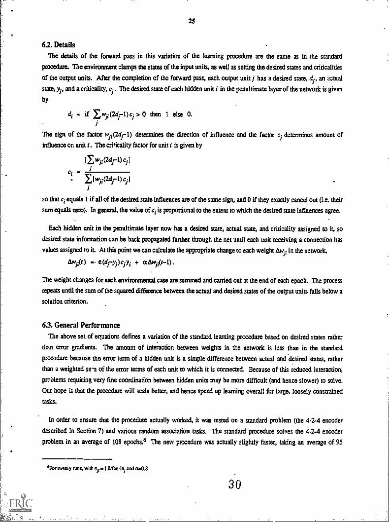
6.2. Details
The details of the forward pass in this variation of the learning procedure are the same as in the standard
procedure. The environment clamps the states of the input units, as well as setting the desired states and criticalities
of the output units. After the completion of the forward pass, each output unit j has a desired state, di, an actual
state, yi, and a criticality, ci. The desired state of each hidden unit i in the penultimate layer of the network is given
by
di = if li wii (2di-1) ci > 0 then 1 else 0.i
The sign of the factor w.ii(2di--1) determines the direction of influence and the factor ci determines amount of
influence on unit i. The criticality factor for unit i is given by
I I wii (24 1) ci I
ci = .r.,Llw ii(2d 1-1) c ji .i
so that ci equals 1 if all of the desired state influences are of the same sign, and 0 if they exactly cancel out (i.e. their
sum equals zero). In general, the value of ci is proportional to the extent to which the desired state influences agree.
Each hidden unit in the penultimate layer now has a desired state, actual state, and criticality assigned to it, so
desired state information can be back propagated further through the net until each unit receiving a connection has
values assigned to it. At this point we can calculate the appropriate change to each weight LW" in the network,
Awls (t) .. e(dryi)ciyi + aAwji(t-1).
The weight changes for each environmental case are summed and carried out at the end of each epoch. The process
repeats until the sum of the squared difference between the actual and desired states of the output units falls below a
solution criterion.
6.3. General Performance
The above set of equations defines a variation of the standard learning procedure based on desired states rather
tiisn error gradients. The amount of interaction between weights in the network is less than in the standard
procedure because the error term of a hidden unit is a simple difference between actual and desired states, rather
than a weighted su-n of the error terms of each unit to which it is connected. Because of this reduced interaction,
problems requiring very fine coordination between hidden units may be more difficult (and hence slower) to solve.
Our hope is that the procedure will scale better, and hence speed up learning overall for large, loosely constrained
tasks.
In order to ensure that the procedure actually worked, it was tested on a standard problem (the 4-2-4 encoder
described in Section 7) and various random association tasks. The standard procedure solves the 4-2-4 encoder
problem in an average of 108 epochs.6 The new procedure was actually slightly faster, taking an average of 95
6For twenty tuns, with ex . 1.0/fan-ini and a0.8
30
26
epoch.; when it solved the task. Unfortunately, it would fail to solve the task occasionally, settling into a state in
which both hidden units essentially represented the same subportion of the task. This is an example in which the
reduced interaction prevented the network from solving a task requiring a particular relationship between the hidden
units.
On tasks involving learning random binary associations of length 10, the new procedure solved the task every
time, but was significant slower than the standard procedure. Each procedure was run on a fully interconnected
network with 10 input units, 10 hidden units, and 10 output units. On a task with 10 association pairs, the new
procedure took an average of 219 epoch, compared with 100 epochs for the standard p° 3cedure.
Once the viability of the new procedure was established, we tested it on a task that the standard one cannot
solvewhat might be called the 1-10x1-1 encoder problem. The network has a single input unit, a single output unit,
and ten hidden layers, each containing a single unit that is connected to the units in the adjacent layers. The task is
for the output unit to duplicate the state of the input unit. The standard procedure fails on this tack because the error
gradient is greatly reduced as it is back propagated, so that the weights in the lower layers receive negligible
information on how to change. In contrast, desired state information does not become weaker as it is passed back
through the network, and so the new procedure should be able to solve the task. In fact, it took an average of only
115 epochs to solve?
6.4. Scaling Performance
Since our original motivation for formulating this variation of the learning procedure was to develop a Teaming
procedure that scaled well, we compared the two procedures on how well they scaled with the addition of hidden
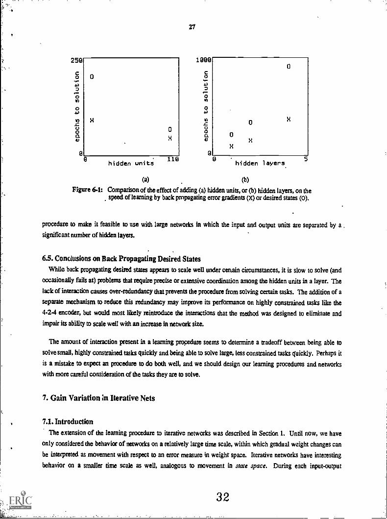
units to a single layer, and with the addition of hidden layers. Figure 6-la shows results for three-layered networks
with either 10 or 100 hidden units on the task of 10 random binary associations of length 10. While the new
procedure takes more epochs to solve the task in general, its performance improves to a greater extent with the
addition of hidden units than does the standard procedure. With larger, similarly structured tasks, the new procedure
might indeed perform better.
However, the addition of hidden layers impairs the performance of the new procedure significantly more than the
standard procedure (see figure 6-1b) This is somewhat surprising, given the success of the ix.w procedure on the
1-10x1-1 encoder problem. Its occasional failure on the 4-2-4 encoder problem suggests a reason for its poor
scaling behavior with multilayered networks. The pressure for hidden units in a layer to differentiate function is
reduced in the new procedure as a result of the reduced interaction between the units. As the number of layers in a
network is increased, information from the output units exerts less differentiating influence on early layers. As a
result, hidden units in early layers become overly redundant at the expense of being able to encode some information
necessary to solve other aspects of the task. It seems that this over--ulundancy is difficult to unlearn and slows the
solution of the task when using a multilayered network. An additional pressure on the hidden units in a layer to take
on separate functions (perhaps some sort of decorrelation, or lateral inhibition) would have to be added to the
?With a very large value of e, for example 10.0, the new procedure takes only 32 epochs on average to solve the 1-10x1-1 encoder problem.
31.
250
c0:.;D
0to
04.)
toz0O0.4)
0
0
X
0
X
0hidden units
110
27
1000
0
0
X
0
V
0
X
0hidden layers
5
Figure 6-1: Comparison of the effect of adding (a) hidden units, or (b) hidden layers, on thespeed of learning by back pmpagating error gradients (x) or desired states (0).
procedure to make it feasible to use with large networks in which the input and output units are separated by a
significant number of hidden layers.
6.S. Conclusions on Back Propagating Desired States
While back propagating desired states appears to scale well under cenain circumstances, it is slow to solve (and
occasionally fails at) problems that require precise or extensive coordination among the hidden units in a layer. The
lack of interaction causes over-redundancy that prevents the procedure from solving certain tasks. The addition of a
separate mechanism to reduce this redundancy may improve its performance on highly constrained tasks like the
4-2-4 encoder, but would most lately reintroduce the interactions that the method was designed to eliminate and
impair its ability to scale well with an increase in network size.
The amount of interaction present in a learning procedure seems to determine a tradeoff between being able to
solve small, highly constrained tasks quickly and being able to solve large, less constrained tasks quickly. Perhaps it
is a mistake to expect an procedure to do both well, and we should design our learning procedures and networks
with more careful consideration of the tasks they are to solve.
7. Gain Variation ;n Iterative Nets
7.1. Introduction
The extension of the learning procedure to iterative networks was described in Section 1. Until now, we have
only considered the behavior of networks on a relatively large time scale, within which gradual weight changes can
be interpreted as movement with respect to an error measure in weight space. Iterative networks have interesting
behavior on a smaller time scale as well, analogous to movement in state space. During each input-output
32
28
presentation the global state of the network varies as the units in the network interact with each other to reach some
final (possibly stable) global state.. Since we will mainly be concerned with iterative nets that settle into a stable or
nearly stable state, we will refer to the shorter time scale as a settling. The results developed so far for the learning
procedure have concentrated on effects over the larger time scale. It is also possible to investigate the variation of
parameters over the smaller time scale. One such parameter that may be varied as the network settles is the amount
of gain at the inputs of individual,units. Motivation for such study may be found in work which has investigated
gain effects in other types of networks.
The continuous valued units used in the back propagation networks can be related to the stochastic units used in
Boltzmann Machines [Hinton 83, Ackley 85]. The sigmoid function used to determine the output value of the
continuous unit is the same function used to determine the probability distribution of the state of a binary-valued
Boltzmann unit: The output of the continuous unit can be interpreted as representing the expected value of an
ensemble of Boltzmann units, or equivalently, the time average of a single unit, if no other units change state. This
relationship between the probability distribution of the state of a unit in a Boltzmann Machine and the value of the
output of a continuous unit in a back propagation net allows one to relate gain variation to simulated
annealing [Kirkpatrick 83]. In a Boltzmann Machine the probability of a unit having output 1 is
1
P.t "` serf1 + e a
where T is the annealing temperature, and the energy term is simply a weighted sum of the inputs to a unit. In a
back propagation net with variable gain the output of a unit is
Yi1ag
1 + e-GE w,iy,
i
It has been shown that simulated annealing is a good method to improve the ability of networks of stochastic units
to settle on a globally optimal solution [Kirkpatrick 83, Ackley 85]. Since gain in iterative networks plays a role
analogous to the inverse of temperature in Boltzmann Machines, allowing the system to vary the gain as it settles
may also improve the convergence of iterative networks.
Stronger support for gain variation in iterative nets comes from recent work by Hopfield and Tank [Hopfield 85].
The authors examined the ability of networks of non-linear analog units to settle into a better than random solution
to the Traveling-Salesman Problem. The units in their network are modelled by analog rather than digital
components, producing an input-output relation that is a continuous function of time. However, the input-output
relation is defined by a sigmoid applied deterministically to the weighted sum of the inputs. Thus each unit in a
Hopfield and Tank net is very similar to a unit in a back propagation net.
Hopfield and Tank show that the solution reached by their networks with a fixed gain uo is equivalent to the
effective field solution of a thermodynamic equilibrium problem with an effective temperature kT = uoat, where T
is temperature, k is a proportionality constant, and T is a parameter representing the time over which the input is
33
?
29
integrated. Furthermore, the effective field solution when followed from high temperatures will lead to a state near
the thermodynamic ground state (i.e. a state near the global energy minimum of the system). The authors note that
A computation analogous to following effective field solutions from high temperatures can be performed by slowlyturning up the analog gain from an initially low value [Hopfield 85, p. 150].
[Hopfield 85] provides some insight into why it is helpful to start with low gain. If the outputs of the units are
confined to the range (0,1] then the possible states of the system are contained within an n-dimensional hypercube,
where n is the number of output units. In the high gain limit, the stable states of the network (i.e. minima of the
energy function) are located at the corners of the hypercube. With lower gain, the stable states migrate towards the
center of the volume defined by the hypercube. As they move inwards, minima that are distinct with higher gain
merge. Each minimum of the low gain system represents a whole set of similar high gain minima. By starting at
low gain it is therefore possible to select a set of promising high gain minima, without yet becoming committed to a
particular minima within that set. Further search refines this set as the gain is increased.
Hopfield and Tank's results indicate that gain variation, and in particular a slow increase in gain during settling,
can improve the performance of iterative nets, but care must be taken in extending these results to cover iterative
back propagation nets. The nets investigated by Hopfield and Tank had symmetric connections. For such networks
there is a global energy function that determines the behavior of the network, and the stable states of the network are
minima of this energy function [Hopfield 82]. No such conditions hold for the general asymmetric nets used by
back propagation.8 In addition, the Hopfield and Tank nets were allowed to settle until they reached equilibrium,
.while the typical iterative back propagation net is only allowed to settle for a fixed number of time steps and may
not reach equilibrium. Finally, the Hopfield and Tank nets have a fixed set of weights, while the weights of the
iterative back propagation net change between settling,s.9 Although this difference is not directly relevant to the
application of gain variation to the networks, it does raise interestizg questions about whether improving
performance in the state space will affect search in the weight space.
Empirical results also suggest that gain variation may be useful in iterative back propagation nets. In most
experiments a problem is considered solved when the global error measure drops below some specified criterion.
Further improvements are still possible once this criterion is reached, and often these improvements are obtained by
increasing the magnitude of all weights in the network. This is equivalent to raising the gain.
In what follows we present some results of investigations of gain variation in iterative networks using the back
propagation procedure. Recall that for every iterative net with a finite number of time steps in which to settle there
is an equivalent layered net in which each lager represents a separate time step (see figure 1-2). In a standard
iterative net, the input to a unit at each time step is a weighted sum of the outputs of units in the previous time step
(or previous layer in the equivalent layered net). The corresponding weights in each layer (i.e. time step) of the
network are constrained to be identical.
slt is important not to confuse the global energy function that determines the stable states of a network as it settles with the global errorfunction used to guide the search fora good set of network weights.
9The set of weights is held constant within the shorter time scale of a settling, but is varied over the longer time scale.
34
ir
.
30
Q 0 O*
Multiplicativegain terms foreach iteration
*W2 W4. 0==W1
W3
A simple iterative net thatis run for three iterations An equivalent layered net
Figure 7-1: An iterative net and the equivalent layered net, with gain variation.
In networks with gain variation this model is extended slightly. The extension is most easily illustrated by
reference to the equivalent layered network representation. A multiplicative global gain term is defined for each
layer of the net (see figure 7-1). The input to each unit is now a weighted sum of the outputs of units in the previous
layer times the global gain term for that layer. The corresponding weights in each layer are identical, as before, but
the global gain is allowed to vary across layers. Translating back to the iterative net terminology, the gain is
allowed to vary across time steps as the network settles.
7.2. Implementation of Gain Variation
The optimal gain variation in an iterative net is to be "learned" by the system by applying the back-propagation
procedure to the gain terms of each time step. This approach is equivalent to performing a gradient descent search
for the optimal values of the gain terms in the error measure defined by Eq. 3. In Section 1 we derived the gradient
of this error measure with respect to each weight in the network (see Eq. 5).
To extend this development to networks with variable gain it is easiest to consider the gain to be a multiplicative
term applied to the input for each unit.
x.ht = GI wiiyiat
where Gt represents the global gain at time t, and xj.1 is the summed input to unit j. This is the same input as in a
31
normal iterative net except for the multiplicative gain term (c.f. Eq. 1). The wfi terms are constant for all time steps
of the settling, while the GI term and yi4 terms vary across the settling.
It is possible to derive expressions for the gradient of the error with respect to each wfi and with respect to each
Gt. For the wfi terms application of the chain rule yields
aE aE arpXI
Iaxj,
Evaluating the derivative of the total input with respect to each weight yields
aE v aEft t
We must sum the contributions to the error gradient from each time step in order to maintain the equivalence of
corresponding weights across time steps, as pointed out in Section 1.4.
To determine the gradient of the error with respect to each gain term we must sum the contribution of each unit
for that time step.
aE EaE ax11ac,
These derivatives must be evaluated separately for each time step in order to determine the optimal gain variation
during a settling.
8E 8EBoth -6-; and are averaged over all input cases before the values of Gi or wfi are updated. In addition, the wfi
gradients are also averaged over iterations, while a separate gradient must be maintained for each time step for the
gain terms.
We use the standard acceleration method in modifying each wfi (see Eq. 7), but the gain terms are modified using
a strict gradient descent method without the acceleration term.
AGt eG aEact
73. Experimental Results
Two results were expected when gain variation was implemented in the iterative nets:
1. Networks would develop a gain schedule in which an initially small gain would be increasedmonotonically over the settling period.
2. Networks would reach a solution to a problem in fewer iterations of the learning procedure.
The first expectation is based on the work on annealing in stochastic networks and Hopfield and Tank's work.
The second expectation is based on the fact that a network using a suitable gain schedule can outperform a network
with the identical set of weights but without gain variation. AlloWing the network to vary the gain as it settles
improves the ability of the network to find a stable state close to the global optimum. This effect can have an
36
32
indirect influence on the weight space search since if a better solution can be found for a given weight set, then less
fine tuning of the weights will be required to reach the solution criterion. Since the number of stable states (hence
possible local optima) increases with network size, these effects should be more noticeable with large networks.
Two different tasks were used to investigate the effects of gain variation. The first task was the 4-1-4 encoder
problem, very similar to the 4-2-4 encoder described in [Ackley 85]. The 4-2-4 network has three layers, with 4
units in each of the input and output layers and 2 units in the hidden layer. Each hidden unit is connected to all of
the input units and all of the output units. The task of the network is to learn a mapping such that when a single
input unit is turned on, the corresponding output unit will be turned on.1° The 4-1-4 network differs from the 4-2-4
network in that only a single hidden unit is used, and each output unit is connected in both directions with each other
output unit (see figure 7-2). This interconnectivity allowed the output units to learn to mutually inhibit each other,
thus forming a winner-take-all network [Feldman 82]. The network was presented with each input vector and then
allowed 5 cycles to settle before the output was examined and an error measure calculated. As with the layered
networks, error gradients were averaged over all input cases before updating the weights.
Output units
Hidden unit
Input units
Figure 7-2: The 4-1-4 encoder network.
Twenty sets of runs were performed. In each run the weight step and momentum were held constant (e=0.1,
a.0.9) while the gain step, CG, was varied systematically from 0.0 to 0.06 in steps of 0.002. Each run began with a
different set of small random weights. The results supported our predictions. Without gain variation the network
required an average of 2269 epochs to fmd a solution; with gal:, variation the average was reduced to 566 epochs.11
Figure 7-3 presents the number of epochs required to reach solution versus the gain step size for a typical run. Note
that the graph tends to decay exponentially. Intrcducing even a moderate amount of gain variation can yield
significant improvements, but the amount of improvement rapidly levels off. Figure 7-4 represents a typical gain
10The hidden units must use their states to encode which of the 4 input units is on. If units were binary, then the code learnedwould have tomake optimal use of the bandwidth provided by the two hidden units.
"The ranges were 1652 to 3867 epochs without gain variation, 155 to 1000 with gain variation.
37
33
schedule learned by the system. The basic shape of the gain schedule was identical in all test runs. As expected thz
system learns to increase the gain as the system settles. With only five data points it is not possible to fit any
particular function to the form of the gain schedule with any great degree of accuracy.
e4000034 35002M4u 3000atuo. *
2500*
2000
5000.00 0.01 0.02 0.03 0.04 0.05 0.06
Gain Step
Figure 7-3: Graph of number of epochs to solution vs. gain step size for the 4-1-4 network.
c 3.5es
3.0
2.5
2.0
1.5
1.
*
*
**
I 2 3 4 5Time Step
Figure 7-4: Typical gain schedule for the 4-1-4 network.
A second set of test runs was performed on a 10-10-10 network in which the learning task required associating 15
10-bit random vector pairs. In this case both the output and hidden units were fully interconnected (see figure 7-5),
and the network was allowed 11 cycles to settle before its output was examined. Ten sample runs were performed in
38
Output units
Hidden units
Input units
34
10 units
Figure 7-5: The 10-10-10 network used for the association of 10-bit random vector pairs.
c 2.8Uei
2.4
2.2
2.0
1.8
1.8
1.4
1.2*
*
0.8
*
*
*
8 9 10Time Step
Figure 7-6: Typical gain schedule learned for the 10-10-10 network.
39
3S
which e and a were held constant (e0.05, co.0.8) and eG was varied systematically. The results again supported
predictims. A typical gain schedule learned by the network is shown in figure 7-6.
In this case the average number of epochs to find a solution was 263 without gain and 184 with gain.12 The
improvement achieved with gain variation in this problem is not as significant as with the 4-1-4 problem, and there
was considerable overlap in the values obtained with and without gain. (In two of the sample runs the solution was
actually found slightly faster with no gain variation at all.) The reason for this difference may be the greater amount
of fine tuning required to find a satisfactory solution for the 4-1-4 nets,
An examination of the gain schedules learned in both the 4-1-4 and 10-10-10 networks reveals some peculiar
properties. In particular, the gain in the last two time steps of the settling is much larger than in any of the other
time steps. This effect is more apparent in the 4-1-4 networks and is believed to be caused by a combination of two
factors:
1. Tit network architecture.
2. The generation of an external error signal only after the network has settled.
In order to understand the effects of these factors, consider figure 7-7, which presents a view of a 4-1-4 network
exploded in time. Each row of the figure represents the state of a network at a point in time, the distance between
rows representing a single time step. The bottom row is the beginning of a settling and the top row represents the
end of the settling. Going :Oro s s a row we see that the 4-1-4 net can be considered as having 3 layers of units (input,
hidden and output). During the settling, signals flow either along columns, for interconnected units in the same
layer, or along the diagonals, for interconnected units in different layers. The history of the network is defined as
the sequence of states the network goes through during a single settling. Thus there is a history entry for each row in
figure 7-7. These histories are stored locally by each unit. The backward pass for an iterative net starts with the
history entry for the final time step of the settling and propagates error gradien backwards toward the history entry
for the first time step of the settling. If we consider each row of figure 7-7 as a history entry, with the entry for the
first time step of the settling at the bottom, and that for the last at the top, then the backward pass starts at the top of
the figure and works its way toward the bottom (i.e. in the direction opposite to that indicated by the arrows on the
figure). As in the forward pass, signals only propagate vertically or along diagonals. It is important to note that
signals moving along diagonals are moving both between physical layers and between time steps.
Consider again the exploded 4-1-4 network. Note that since the input units can ow:' communicate with the output
units through the middle layer of units, there will be a two time step propagation del; y for signals to move between
the input and output layers in both the forward and backward pass. As error gradients are propagated back to earlier
history entries, the magnitudes are greatly reduced. In a network in which the actual output is compared to the
desired output only during the last time step of the settling there is a large external error input introduced at this last
time step. This error signal will propagate back to the input unit histories corresponding to the two time steps
immediately prior to the final time step. For all history entries prior to that: last two, the error gradients will be
I2These results are slower than for a corresponding problem with a layered network. This is attributed to different values for a and a differentset of input vectors.
40
iteration 5
iteration 4
iteration 3
iteration 2
iteration 1
36
Input units
0 0 0 0
Hiddenunit Output units
O 0000
0 0000
O 0000
O 0000
O 0000
O 0000
0000
0000
0 0 0 0
0000
0000Figure 7-7: An exploded time view of a 4.1-4 network. Each row correspond
to a time step of the settling, with the bottom row being thebeginning. Each ow represents a set of connections.
residual error propagated back from error terms calculated for the last two time steps. These residual error gradients
are smaller than the direct external errors. Recall that the gradient of the gain term is calculated by summing the
gradients of all weights for each time step. The sum of the error gradients for the last two time steps will be much
larger than for the other time steps. This will tend to drive the gain change more rapidly for these two steps, leading
to the effect of much larger gains for these last two steps.
To test this hypothesis, two further groups of experiments were performed. In the first, a set of networks in which
the propagation delays could be modified systematically were trained on a standard encoder problem. Each of these
networks had 4 input units, 4 output units and n groups of 4 hidden units arranged so signals from the input units
had to travel through all n groups of hidden units before reaching the output units. We call thee 4-n4-4 networks
(see figure 7-8). If .1 propagation delays through the network affected the gain gradients as suggested then there
41
37
should bea linear-relationshipbetween the-number of groups-of hidden units and the number of time steps with
large gains. Such a relationship was found for n.1 to 4. In general, if there were n groups of hidden units then the
last n time steps all had gains larger than the other time steps. As n was increased this step effect in gain became
less pronounced.
Outputunits
n Hiddenlayers
Inputunits
Figure74: A 4-n4-4 network.
Fullyinterconnected
layers
The second group of experiments used a task in which the error for the output units was not always calculated
during the final time step. The network consisted of 10 input units, 5 hidden units and a single output unit. Each
hidden unit was connected to all 10 input units and also to the other 4 hidden units. The output unit was only
connected to the S hidden units. The task the network had to learn required setting the state of the output unit to be 1
after a certain delay from the time the network started to settle. Each input unit corresponded to one of 10 different
required delays, and only one input unit was on at a time. Since in this task the external error signals were well
distributed over all of the time steps, there should be no sudden step towards the end of the settling process. The
gain variation schedule learned for this problem showed no step in the gain response, as expected (see figure 7-9).
However the gain schedule also did not exhibit the characteristic increase of gain over the settling period. Rather
the gain tended to peak then decay during the settling period.
All of the results discussed in this section have been based on netwoiks with asymmetric connections. The results
42
e 2.0
01.8
1.6
1.4
1.2
1.
0.8
0.6
0.41 2 3 4 5 6 7 .8 9 10
77me Shop
38
Figure 7.9: Gain schedule for the variable delay task.
of Hopfield and Tank fllopfield 853, which this work has extended, were based on symmetric networks that have an
energy function which governs their settling behavior: We investigated the effects of symmetrical connections by
repeating the 4-1-4 encoder and 10-10-10 association problems using networks with symmetric connections. The
results for the symmAric networks were identical to the results obtained for the asymmetric networks in terms of the
effects of gain variation. It was noted that the symmetric networks required more epochs to learn the same tasks.
This is may be due to the greater number of connections and correspondingly higher fan-in for each unit (see
Section 4), rather than a direct result of synunetly.
Several other experiments were performed to compare the performance of the learned gain schedules to schedules
designed by hand. The schedules investigated provided linear, quadratic and exponential growth in gain over the
settling period of a 4-1-4 encoder. None of these hand-tooled schedules could outperform the learned schedules, and
most did not perform as well. The performance of these prespecified schedules varied from test case to test case,
although both the quadratic and exponential schedules consistently outperformed the linear schedule. When any of
these schedules were reversed so that gain tended to decrease during the settling the learning performance was
degraded severely. In particular, the learning procedure became prone to becoming stuck in sub-optimal states, and
often would become unstable and cease to converge on a solution, by moving in directions which led to increases in
the error criterion.13
These experimental results support the view that gain variation can improve the performance of iterative
networks. However, it is also apparent that the degree of improvement is problem dependent. Further research '3
"Similar behavior is sometimes noted when weight decay is applied to a network.
39
required to determine which characteristics of a problem (and the associated state space) indicate that a problem can
bene.5 nbstantially from gain variation.
44
40
References
[Ackley 85] Ackley DR., Hinton G.E. and Sejnowski TJ.A learning algorithm for Boltzmann Machines.Cognitive Science 9(2):147-169, 1985.
[Feldman 82] Feldman J.A. and Ballard D.H.Connectionist models and their properties.Cognitive Science 6:205-254, 1982.
[Hinton 83] Hinton G.E. and Sejnowski Ti.Optimal perceptual inference.In Proceedings, IEEE conference on Computer Vision and Pattern Recognition. Washington DC,June, 1983.
[Hopfield 82] Hopfield J.J.Neural networks and physical systems with emergent collective computational abilities.Proceedings of the National Academy of Sciences 79:2554-2558, 1982.
[Hopfield 85] Hopfield J.J. and Tank D.W."Neural" computation of decisions in optimization problems.Biological Cybernetics 52:141-152, 1985.
[Kirkpatrick 83] Kirkpatrick S., Gelatt C.D. and Vecchi M.P.Optimization by simulated annealing.Science 220:671-680, 1983.
[Le Cun 85] Le Cun Y.Une prodedure d'apprentissage pour reseau a seuil assymetrique (A learning scheme forasymmetric threshold network).In Cognitiva 85. Paris, France, June, 1985.
[Le Cun 86] Le Cun Y.Learning process in an asymmetric threshold network.In E. Bienenstock, F. Fogelman and G. Weisbuch (editors), Disordered systems and biologicalorganization. Springer Verlag, New York, 1986.
[Rumelhart 86] Rumelhart D.E., Hinton G.E. and Williams RJ.Learning internal representations by error propagation.In D.E. Rumelhart, J.L. McClelland and the PDP research group (editors), Parallel distributedprocessing: Explorations in the microstructure of cognition. Volume I: Foundations. MIT Press,Cambridge, MA, 1986.
[Torre 86] Torre V. and Poggio T.A.On edge detection.IEEE Transactions on Pattern Analysis and Machine Intelligence PAMI-8(2):147-163, March, .
1986.
45
1986/03/20
Distribution List 1UCSD/Elman & McClelland] Nit 667-483
Dr. Phillip L. Ackerman Dr. Jackson RealtyUniversity of Minnesota Department of PsychologyDepartment of Psychology University of CaliforniaMinneapolis, MN 55455 Los Angeles, CA 90024
Air Force Human Resources Lab Dr. Alvah ittntrAFRIL/RFO Naval Biodynamics LaboratoryBrooks APB, TX 78235 New Orleans, LA 70189
AFOSR, Dr. John BlackLife Sciences Directorate Yale UniversityBolling Air Force Ease Sox 11A, Tale Station
Vashington, DC 20332 Nev Haven, CT 06520
Dr. RoberLAhlers Dr. Arthur S. BlaivesCode N711 Code N711Boman Factors Laboratory Naval Training Equipment CenterNAVTRAEQUIKIN Orlando, FL 32813Orlando, FL 32813
Dr. Cordon N. loverDr. Ed Aiken Department of PsychologyNavy Personnel R&D Center Stanford UniversitySan Diego, CA 92152 Stanford, CA 94306
Dr. Earl A. Alluisi Dr. Robert BreauxNO, AFHRL (APSC) Code N-095RBrooks TX 78235 NAVTRAEGUIPCEN
Orlando, FL 32813Dr. Jons AndersonBrown University Dr. Gail CarpenterCenter for 6e.=.! Science Northeastern UniversityProvidence, RI 02512 Department of Mathematics, 504LA
360 Huntington Avenue
Dr. John R. Antirson Boston, MA 02115Department ot PsychologyCarnegie- Mellon University Dr. Pat CarpenterPittsburgh, PA 15213 Carnegie-Mellon University
Department of PsychologyDr. Nancy S. Anderson Pittsburgh, PA 15213Department of PsychologyUniversity of Maryland Chair, Department ofCollege Park, MD 20742 Psychology
College of Arts and SciencesTechnical Director, MI Catholic University of
5001 Eisenhover Avenue AmericaAlexandria, VA 22333 Vashington, DC 20064
Dr. Alan Baddeley Dr. Fred Chang
Medical Research Council Navy Personnel R&D CenterApplied Psychology Unit Code 5115 Chaucer Road San Diego, CA 92152Cambridge CB2 2EFENGLAND
1986/03/20
Distribution List 1UCSD/Elman I. McClelland] NR 667-483
Dr. David E. Clement Dr. R. K. DismukesDepartment of Psychology Associate Director for LifeUniversity of South Calorina ScienceColumbia, SC 29208 AFOSR
Bolling APBVashington, DC 20332
Dr. Charles CliftonTobin Hall Dr. Emanuel Donchin
Department of Psychology University of IllinoisUniversity of Department of Psychology
Massachusetts Champaign, IL 61820Amherst, MA 01003
Defense TechnicalDr. Michael Coles Information CenterUniversity of Illinois Cameron Station, Bldg 5Department of Psychology Alexandria, VA 22314Champaign, IL 61820 Attn: TC
(12 Copies)Dr. John J. CollinsDirector, Field Research Dr. Ford Ebner
Office, Orlando Brown UniversityNPRDC Liaison Officer Anatomy DepartmentNTSC Orlando, FL 32813 Medical School
Providence, RI 02912Dr. Stanley CollyerOffice of Naval Technology Dr. Jeffrey SloanCode 222 University of California,800 N. Quincy Street San DiegoArlington, VA 22217-5000 Department of Linguistics, C-008
La Jolla, CA 92093Dr. Leon CooperBrown University Dr. Villa* EpsteinCenter for Neural Science University of VisconsinProvidence, RI 02912 V. J. Brogden Psychology Bldg.
1202 V. Johnson StreetCAPT P. Michael Curran Madison, VI 53706Office of Naval Research800 N. Quincy St. ERIC Facility-AcquisitionsCode 125 4833 Rugby AvenueArlington, VA 22217-5000 Bethesda, MD 20014
Bryan Dallman Dr. K. Anders EricssonAFHRL /LRT University of ColoradoLowry AFB, CO 80230 Department of Psychology
Boulder, CO 80309Dr. Joel DavisOffice of Naval Research Dr. V. E. EvansCode 1141NP Hubbs Sea Vorld Institute800 North Quincy Street 1720 S. Shores Rd.Arlington, VA 22217-5000 Mission Bay
Sin Diego, CA 92109
46
1986/03/20
Distribution List IUCSD/Elman i McClelland) NR 667-483
Dr. Martha Farah Dr. Daniel GopherDepartment of Psychology Industrial EngineeringCarnegie-Mellon University ManagementSchenley Park TICHNIONPittsburgh, PA 15213 Haifa 32000
ISRAEL
1986/03/20
Distribution List IUCSD/Elman i McClelland) NR 667-483
Dr. Ray Hannapel Chair, Department ofScientific and Engineering Psychology
Personnel and Education The Johns Uopkins UniversityNational Science Foundation Baltimore, MD 21218Vashington, DC 20550
Dr. Marcel Just
Dr. Jerome A. Feldman Stevan Harnad Carnegie-Mellon University
University of Rochester Dr. Sherrie Cott Editor, The Behavioral and Department of Psychology
Computer Science Department AFIRL/NOCU Brain Sciences Schenley Park
Rochester, NY 14627 Brooks APB, TX 78235 20 Nassau Street, Suite 240 Pittsburgh, PA 15213Princeton, NJ 08540
J. D. Fletcher Jordan Grafman, Ph.D. Dr. Daniel Kahneman
9931 Corsica Street Department of Clinical Dr. Steven A. Hillyard The University of British Columbia
Vienna VA 22180 Investigation Department of Neurosciences Department of Psychology
Dr. John R. FroderiksenValter Reed Army Medical Center6825 Georgia Ave., N. V.
University of California,San Diego
1154-2053 Main MallVancouver, British Columbia
Bolt Beranek i Newman Vashington, DC 20307-5001 La Jolla, CA 2093 CANADA V6T 127
50 Moulton StreetCambridge, NA 02131 Dr. Richard I. Granger Dr. Geoffrey Hinton Dr. Demetrios Karis
Department of Computer Science Carnegie-Mellon University Grumman Aerospace Corporation
Dr. Michaels Gallagher University of California, Irvine Computer Science Department MS C04-14
University of North Carolina Irvine, CA 92717 Pittsburgh, PA 15213 Bethpage, NY 11714
Department of PsychologyChapel Hill, NC 27514 Dr. Vayne Gray Dr. Jim Hollan Dr. Milton S. Katz
Army Research Institute Intelligent Systems Group Army R h Institute
Dr. Michael Genesereth 5001 Bisenhover Avenue Institute for 5001 Eisenhower Avenue
Stanford University Alexandria, VA 22333 Cognitive Science (C-015) Alexandria, VA 22333
Computer Science Department UCSD
Stanford, CA 94305 Dr. Villiam Greenough La Jolla, CA 92093 Dr. Steven V. Keele
University of Illinois Department of Psychology
Dr. Don Gentner Department of Psychology Dr. John Holland University of Oregon
Center for Human Champaign, IL 61820 University of Michigan Eugene, OR 97403
Information Processing 2313 East EngineeringUniversity of California Dr. Stephen Grossberg Ann Arbor, MI 48109 Dr. Vendy Kellogg
La Jolla, CA 92093 Center for Adaptive Systems IBM T. J. Vatson Research Ctr.
Room 244 Dr. Keith Holyoak P.O. Box 218
Dr. Claude Chet 111 Cummington Street University of Michigan Yorktown Heights, NY 10598
Center for Neurobiology and Boston University Human Performance CenterBehavior Boston,'MA 02215 330 Packard Road Dr. Scott Kelso
722 V. 168th StreetNew York, NT 10032 Dr. Muhammad K. Habib
Ann Arbor, MI 48109 Haskins Laboratories,270 Crown Street
University of North Carolina Dr. Earl Hunt New Haven, CT 06510
Dr. Gene L. Cloys Department of Biostatistics Department of Psychology
Office of Naval Research Chapel Hill, NC 27514 University of Vashington Dr. David Klahr
Detachment Seattle, VA 98105 Carnegie-Mellon University
1030 E. Green Street Dr. Henry M. Halff Department of Psychology
Pasadena, CA 91106-2485 Halff Resources, Inc. Dr. Alice Isen Schenley Park
4918 33rd Road, North Department of Psychology Pittsburgh, PA 15213Dr. Sam Glucksberg Arlington, VA 22207 University of MarylandPrinceton University Catonsville, MD 21228Department of PsychologyGreen HallPrinceton, NJ 08540
48
1986/03/20
Distribution List [UCSD/Elman I McClelland) NR 667-483
Dr. Sylvan Kornblum Dr. Don LyonUniversity of Michigan P. O. Box 44Mental Health R h Institute Higley, AZ 85236205 Vashtenav PlaceAnn Arbor, MI 48109 Dr. James McBride
1986/03/20
Distribution List [UCSD/Elman I McClelland) OR 667-483
Chair, Department of Office of Naval Research,Systems Engineering Cock 1133
U.S. Naval Academy 800 N. Quincy StreetAnnapolis, MD 21402 Arlington, VA 22217-5000
Dr. Stephen KosslynPsychological Corporationc/o Marcourt, Brace,
Dr. David MayonInstitute for Cognitive Science
Office of Naval R h,
Code 1141NPHarvard University Javanovich Inc. University of California 800 N. Quincy Street1236 Villiam James Nall 1250 Vest 6tb Street La Jolla, CA 92093 Arlington, VA 22217-500033 Kirkland St. San Diego, CA 92101Cambiidge, MA 02138
Dr. Jay McClellandDr. Allen NewellDepartment of Psychology
Office of Naval R h,
Code 1142EPDr. David R. Lambert Department of Psychology Carnegie-Mellon University 800 N. Quincy StreetNaval Ocean Systems Center Carnegie-Mellon University Schenley Park Arlington, VA 22217-5000Code 441T Pittsburgh, PA 15213 Pittsburgh, PA 15213271 Catalina BoulevardSan Diego, CA 92152 Dr. Jugs L."McGaugh Dr. Mary Jo Nissen
Office of Naval Research,Code 1142PT
Center for the Neurobiology University of Minnesota 800 N. Quincy StreetDr. Pat Langley of Learning and Memory N218 Elliott Hall Arlington, VA 22217-5000University of California University of California, Irvine Minneapolis, MN 55455 (S Copies)Department of information Irvine, CA 92717and Computer Science Dr. Donald A. Norman Psychologist
Irvine, CA 92717 Dr. Joe McLachlan Institute for Cognitive Science Office of Naval ResearchNavy Personnel R&D Center University of California Branch Office, London'
Dr. Marcy Lansaan San Diego,,CA 92152 La Jolla, CA 92093 Box 39University of North Carolina FPO New York, NY 09510The L. L. Thurston, Lab.Davie Hall 013A
Dr. James McMichaelAssistant for MPT Research,
Director, Training Laboratory,NPRDC (Code 05) Special Assistant for Marine
Chapel Hill, NC 27514 Development, and StudiesNAVOP 0187
San Diego, CA 9c152 Corps Matters,ONR Code 00MC
Dr. Robert Lawler Vashington, DC 20370 Director, Manpover and Personnel 800 N. Quincy St.inforsation Sciences, FRLGTE Laboratories, Inc. Dr. Al MeYrowits
Laboratory,NPRDC (Code 06)
Arlington, VA 22217-5000
40 Sylvan Road Office of Naval R San Diego, CA 92152 PsychologistWaltham, MA 02254 Code 1133 Office of Naval R
800 N. Quincy Director, Human Factors Liaison Office, Far EastDr. Alan N. LesgoldLearning R&D Center
Arlington, VA 22217-5000 & Organizational Systems Lab,NPRDC (Code 07)
APO San Francisco, CA 96503
University of Pittsburgh Dr. George A. Miller San Diego, CA 92152 Dr. Judith OrasanuPittsburgh, PA 15260 Department of Psychology Army R h Institute
Dr. Alan LeshnerGreen HallPrinceton University
Fleet Support Office,NNW (Code 301)
5001 Eisenhower AvenueAlexandria, VA 22333
Deputy Division Director Princeton, NJ 08540 San Diego, CA 92152Behavioral and Neural Sciences Deice PaulsonNational Science Foundation Dr. Tom Moran Library, NPRDC Code 52 - Training Systems1800 C Street Xerox PARC Code P2OIL Navy Personnel RID CenterVashington, DC 20550 3333 Coyote Hill Road San Diego, CA 92152 San Diego, CA 92152
Palo Alto, CA 94304Dr. Gary Lynch Dr. Stellan Ohlsson Dr. James V. PellegrinoUniversity of California Chair, Department of Learning R i D Center University of California,Center for the Neurobiology of Computer Science University of Pittsburgh Santa Barbara
Learning and Memory U.S. Naval Academy 3939 O'Hara. Street Department of PsychologyIrvine, CA 92717 Annapolis, MD 21402 Pittsburgh, PA 15213 Santa Barbara, CA 93106
50 51
1986/03/20
Distribution List (UCSD /Elman 4 McClelland) NR 667-483
1986/03/Z0
Distribution List IUCiD/Elman 4 McClelland( NR 667-483
Department of Computer Science,Naval Postgraduate School
Dr. Gil RicardMail Stop C04-14
Dr. Randall ShumakerNaval Research Laboratory
Dr. Michael T. TurveyHaskins Laboratories
Monterey, CA 93940 Grumman Aerospace Corp. Code 7510 270 Crown StreetBethpage, NT 11714 4555 Overlook Avenue, S.V. New Haven, CT 06510
Dr. Steven Pinker Washington, DC 20375-5000Department of Psychology110-018
Dr. David RumelhartCenter for Rumen Dr. Miriam Schustack
Dr. James TweeddsleTechnical Director
M.I.T. Information Processing Code 51 Navy Personnel 110 CenterCambridge, NA 02139 Univ. of California Navy Personnel R 4 D Center San Diego, CA 92152
La Jolla, CA 92093 San Diego, CA 92152Dr. Martha Poison Headquarters, U. S. Marine CorpsDepartment of Psychology Dr. R. L. Saltzman Dr. Herbert A. Simon Code MPI-20Campus Box 346 Haskins Laboratories Department of Psychology Vashington, DC 20380University of Colorado 270 Crown Street Carnegie-Mellon UniversityBoulder, CO 80309 New Haven, CT 06510 Schenley Park Dr. Wiliam Uttal
Pittsburgh, PA 15213 NOSC, Hawaii LabDr. Peter Poison Dr. Arthur Samuel Box 997University of Colorado Yale University Dr. Kathryn T. Spoehr Konya, HI 96734Department of Psychology Department of Psychology Brown UniversityBoulder, CO 80309 Box 11A, Yale Station Department of Psychology Dr. Kurt Van Lehn
New Haven, CT 06520 Providence, RI 02912 Department of PsychologyDr. Mike Posner Carnegie-Mellon UniversityUniversity of Oregon Dr. Robert Sasmor Dr. Ted Steinke Schenley ParkDepartment of Psychology Army Research Institute Dept. of Geography Pittsburgh, PA 15213Eugene, OR 97403 5001 Sisenhover Avenue University of South Carolina
Alexandria, VA 22333 Columbia, SC 29208 Dr. Beth MarrenDr. Karl Pribram Bolt Beranek 4 Newman, Inc.Stanford University Dr. Walter Schneider Dr. Saul Sternberg 50 Moulton StreetDepartment of Psychology Learning,R4D Center University of Pennsylvania Cambridge, NA 02138Bldg. 4201 -- Jordan Nall University of Pittsburgh Department of PsychologyStanford, CA 94305 3939 O'Hara Street 3815 Walnut Street Dr. Shih-Sung hen
Pittsburgh, PA 15260 Philadelphia, PA 19104 Jackson State UniversityDr. Lynne Rader 1325 J. R. Lynch StreetDepartment of Psychology Dr. Rans-Villi Schroiff Dr. Paul J. Sticha Jackson, MS 39217Carnegie - Mellon University Institut fuer Psychologie Senior Staff ScientistSchenley Park der RVTR Aachen Training Research Division Dr. Douglas WetzelPittsburgh, PA 15213 Jaegerstrasse swischen 17 u. 19 HumRRO Code 12
5100 Aachen 1100 S. Vashington Navy Personnel R&D CenterDr. James A. Reggio VEST GERMANY Alexandria, VA 22314 San Diego, CA 92152University of MarylandSchool of Nedicine Dr. Marc Sebrechts Dr. John Tangney Dr. Barry VhitselDepartment of Neurology Department of Psychology AFOSR/NL University of North Carolina22 South Greene Street Wesleyan University Dolling AFB, DC 20332 Department of PhysiologyBaltimore, MD 21201 Middletown, CT 06475 Medical School
Dr. Richard F. Thompson Chapel Hill, NC 27514Dr. Daniel Reisbetg Dr. T. B. Sheridan Stanioid UniversityDepartment of Psychology Dept. of Mechanical Engineering Department of Psychology Dr. Christopher WickensNew School for Social Research MIT Bldg. 4201 -- Jordan Hall Department of Psychology65 Fifth Avenue Cambridge, NA 02139 Stanford, CA 94305 University ofNew York, NY 10003 Champaign, IL 61820
5253
1986/03/20
Distribution List (UCSD/Elman S. McClelland' NR 667-483
Dr. Robert A. VisherU.S. Army Institute for the
Behavioral and Social Sciences5001 Eisenhover AvenueAlexandria, VA 22333
Dc. Donald VoodvardOffice of Naval ResearchCode 1141NP800 North Quincy StreetArlington, VA 22217-5000
Dr. Vallace Vulfeck, IIINavy Personnel RED CenterSan Diego, CA 92152
Dr. Joe YasatukeAFIIRL/LRT
Lowry APB, CO 80230
Mr. Carl YorkSystem Development Foundation181 Lytton AvenueSuite 210Palo Alto, CA 94301
Dr. Joseph L. YoungMemory i Cognitive
ProcessesNational Science FoundationVashington, DC 20550
Dr. Steven ZornetzerOffice of Naval ResturchCode 1140800 N. Quincy St.Arlington, VA 22217-5000
Dr. Michael J. ZydaNaval Postgraduate SchoolCode 52CKMonterey, CA 93943