DOE Climate Modeling Principle Investigator MeetingPotomac, Maryland

Including albedo affects in IAM scenarios

KATE CALVIN, ANDY JONES, JAE EDMONDS, WILLIAM COLLINS

14 May 2014

PNNL-SA-97327

MOTIVATION

We run two scenarios: RCP 4.5 (UCT) and Rep 4.5 (FFICT)

We hold total CO2 and non-CO2 GHG emissions fixed and run the two scenarios that limit year 2095 radiative forcing to 4.5 Wm-2.

In RCP 4.5 (UCT) we use the original RCP 4.5 land use.

In Rep 4.5 (FFICT) we use the alternative land use—the ONLY thing that is different between the two.

Quantifying the effect of land cover on climate: Results using GCAM & CESM

Calvin et al. (2014). Near-term limits to mitigation: challenges arising from contrary mitigation effects from indirect land-use change and sulfur emissions. Energy Economics.

RCP 4.5 (UCT) Rep 4.5 (FFICT)

Quantifying the effect of land cover on climate: Results using GCAM & CESM

Large change—0.6Wm-2 change in climate forcing from the alternative (Rep 4.5, FFICT) land-use policy assumption.

Change is almost immediate

Time scale of the change from direct physical effects is a decade—in addition to changes in the atmospheric composition of GHGs.

Well within a decadal (up to 40-year) time horizon.

Rep 4.5 (FFICT)

RCP 4.5

(UCT)

Rapi

d Ch

ange

in

PHY

SICA

L Fo

rcin

g Comparison between Rep 4.5 and RCP 4.5Rep 4.5 is shown to be cooler, with rapid transition

under Rep 4.5Jones A et al. (2013) Greenhouse gas policy influences climate via direct effects of land-use change. Journal of Climate 26:3657-3670.

COMPUTING ALBEDO

Forcing is determined by both surface and atmosphere

Steps to calculate forcing in CESM:First we compare surface properties of woody vegetation (forests and/or shrublands) to non-woody vegetation (grassland and/or cropland) in each zone while holding atmospheric forcing constant

Next, we use an offline radiative transfer model (PORT) to compute top-of-atmosphere flux associated with conversion from woody to non-woody vegetation

Incorporating albedo into GCAM

Land conversion:At each timestep, for each region, we compute the amount of land that is converted from woody vegetation to non-woody vegetation in GCAM.

Albedo:The change in albedo is computed by multiplying the albedo factors and the amount of land converted for each region, and then summing over the regions.

This change in albedo is passed into MAGICC.

Albedo Factors by GCAM Region

glob

al n

W/m

2 per

km

2 co

nver

sion

Greatest forcing in Boreal forest zones and Tibetan plateau

Results are function of vegetation, insolation, and clouds

RESULTS

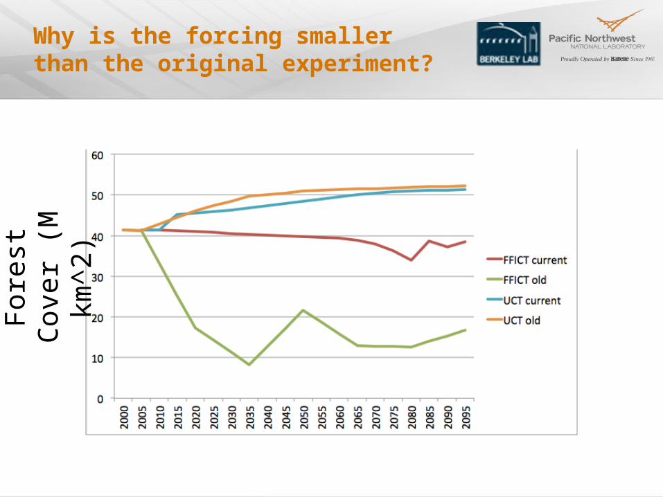
Forcing from Land-Use Change: Revisiting our Original Scenarios

Fore

st C

over

(M

km

^2)

Why is the forcing smaller than the original experiment?

latitude

land

con

vert

ed

(km

^2)

Why is the forcing smaller than the original experiment?

Effect of including albedo in policy targets

Carbon Price

Fossil Fuel Emissions

Land-Use Change Emissions

Albedo Forcing

Forest and Shrub Cover

Bioenergy Crop Area

Some Conclusions

Albedo forcing (and climate effect) of land-use change can be quite significant

Newer GCAM estimates lower rates of deforestation

We can now diagnose albedo change within GCAM

Including albedo in forcing targets feeds back onto energy and land-use systems

Less deforestation in FFICT despite forcing “bonus”

Remaining questions

Given the regional nature of land-use forcing, how do we understand climate implications of equivalent forcing in different locations? Perhaps with pattern scaling?

For impacts research, regional climate is what is critical not global mean temperature rise.

See Jones et al. (2013) GRL paper on differences between albedo and GHG forcing

How different do land cover patterns have to be to induce a significant difference in climate?

We have conducted some scenarios that have differences, but we haven’t systematically tested this.

DISCUSSION