Does Consumer Sentiment Predict Regional Consumption?

WORKING PAPER SERIES

Does Consumer Sentiment Predict Regional Consumption?

Thomas A. Garrett Rubén Hernández-Murillo

and Michael T. Owyang

Working Paper 2003-003C http://research.stlouisfed.org/wp/2003/2003-003.pdf

February 2003 Revised September 2004

FEDERAL RESERVE BANK OF ST. LOUIS Research Division 411 Locust Street

St. Louis, MO 63102

______________________________________________________________________________________

The views expressed are those of the individual authors and do not necessarily reflect official positions of the Federal Reserve Bank of St. Louis, the Federal Reserve System, or the Board of Governors.

Federal Reserve Bank of St. Louis Working Papers are preliminary materials circulated to stimulate discussion and critical comment. References in publications to Federal Reserve Bank of St. Louis Working Papers (other than an acknowledgment that the writer has had access to unpublished material) should be cleared with the author or authors.

Photo courtesy of The Gateway Arch, St. Louis, MO. www.gatewayarch.com

http://www.stlouisarch.com/

1

Does Consumer Sentiment Predict Regional Consumption?1

Thomas A. Garrett

Rubén Hernández-Murillo* Michael T. Owyang

Federal Reserve Bank of St. Louis

Research Division 411 Locust Street

St. Louis, Missouri 63102

(314) 444-8601

JEL Codes: E27, E21, C53

Abstract

This paper tests the ability of consumer sentiment to predict retail spending at the

state level. The results here suggest that, although there is a significant relationship

between sentiment measures and retail sales growth in several states, consumer

sentiment exhibits only modest predictive power for future changes of retail

spending. Measures of consumer sentiment, however, contain additional

explanatory power aside from the information available in other indicators. We also

find that by restricting our attention to fluctuations in retail sales that occur at the

business cycle frequency we can uncover a significant relationship between

consumer sentiment and retail sales growth in many additional states. In light of

these results, we conclude that the practical value of sentiment indices to forecast

consumer spending at the state level is, at best, limited.

1. Introduction

Consumer sentiment is arguably the most cited indicator of current economic conditions, as

it appears to be correlated with the strength of the economy. Following September 11, 2001, the

two most common consumer sentiment indices—the University of Michigan’s Index of Consumer

* Corresponding author: [email protected] 1 The authors wish to thank Marianne Baxter for the use of the Baxter-King bandpass filter software and Jeremy Piger for helpful discussions. Molly Jo Dunn-Castelazo, Kristie M. Engemann, and Deborah Roisman provided research assistance. The views herein are the authors' alone and do not represent the views of the Federal Reserve Bank of St. Louis or the Federal Reserve system.

2

Sentiment (ICS) and the Conference Board’s Consumer Confidence Index (CCI)—fell an average

of 20.9 percent through March 2003, reaching their lowest levels in nearly a decade. During the

same period, real personal consumption expenditures grew by only 4.9 percent, compared to a 6.6

percent rate of growth over the two previous years when consumer sentiment was higher.

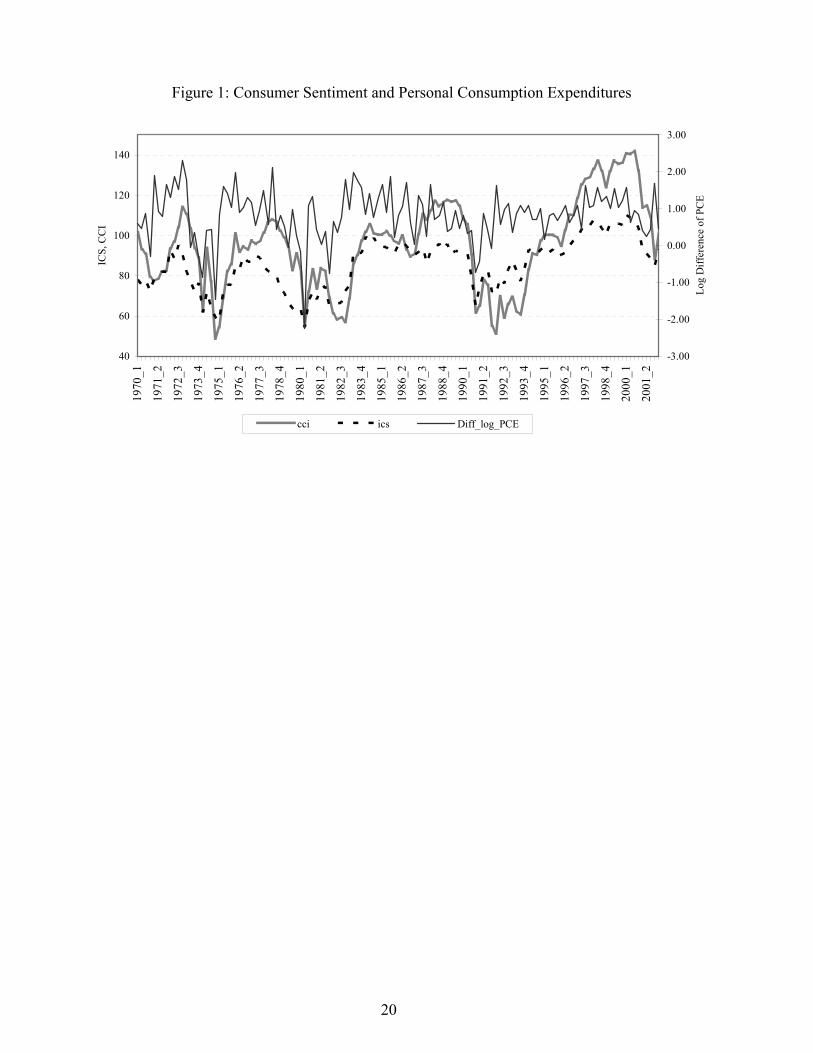
In fact, there is little argument in the academic literature that contemporaneous consumer

sentiment and national consumption expenditure growth are related, as evidenced in Figure 1.

Quarterly data since 1970 reveal an average correlation of 0.43 between personal consumption

expenditures and both sentiment indices. What has been an important and controversial issue in the

literature is the ability of consumer sentiment to forecast future consumption expenditures. Given

that consumption expenditures have a direct correspondence with economic growth, the issue is,

then, whether consumer sentiment can predict economic growth. If consumer sentiment does

predict economic growth, a further question is whether consumer sentiment captures the

perceptions of individuals directly or whether it encompasses the forecasting information contained

in other variables. The answer to this question is of interest, given the timeliness with which the

sentiment indices are released, often ahead of other indicators.2

[Figure 1 about here]

Carroll, Fuhrer, and Wilcox (1994) find that lagged values of ICS significantly explain

nearly 14 percent of growth in real personal consumption expenditures. However, after including

other forecasting variables in their models, the incremental impact of lagged sentiment falls to 3

percent. Bram and Ludvigson (1998) extend the models of Carroll, Fuhrer, and Wilcox (1994) by

considering additional forecasting variables and the CCI in addition to the ICS. They find that the

ICS is no longer a significant predictor of consumption expenditures when interest rate and equity

price changes are included in the models. The CCI, however, did significantly improve the

explanatory power of their forecasting models. This suggests that the CCI and the ICS do not

provide the same forecasting information.

3

These mixed results are echoed in the ability of each sentiment index to forecast production

and employment. Batchelor and Dua (1998) show that the CCI is useful in predicting the 1991

recession, but their results cannot be generalized to other years. Matsusaka and Sbordone (1995)

find that the ICS significantly improves their forecasting model for GNP after considering other

factors such as money growth, interest rates, and government spending. Howrey (2001) obtains a

similar result for forecasts of GDP. Leeper (1992) finds that while the ICS alone is a significant

predictor of industrial production, the inclusion of additional variables eliminates any predictive

power of the ICS.

In contrast with most of the earlier studies, which have explored whether consumer

sentiment predicts national measures of consumption expenditures, in this paper we examine (1)

how well consumer sentiment indices predict retail sales growth at the state level and (2) whether

consumer sentiment measures contain any incremental predictive power about future changes in

consumer spending relative to other indicators of retail sales growth.3 But why attempt to predict

state-level measures at all when suitable aggregate measures are readily available?

A recent paper by Owyang, Piger, and Wall (2004) found that state-level business cycles are

not necessarily synchronous with national cycles. Thus, it is of interest to determine whether and to

what extent consumer sentiment reflects idiosyncratic regional activity versus aggregate conditions.

Further, uncovering a significant relationship between consumer sentiment and retail spending

across states may allow policymakers to extract timely information about regional economic

conditions from consumer sentiment measures. Therefore, we examine whether the relationship

between sentiment and retail spending at the state level is reflected in the national data, and whether

the statistical significance, if any, is driven by a few isolated states.

2 The sentiment indices are some of the earliest economic indicators available at the quarterly frequency. 3 Allenby, Jen, and Leone (1996) find that consumer sentiment forecasts retail fashion sales. The authors used sales data from five specialty divisions of a Fortune 500 retailer.

4

2. Methodology and Data

2.1 Model

The regression model we use to judge the predictive ability of consumer sentiment on state

retail sales growth is:

11

' + K

t-it t tii=

R = + + ZSα γ εβ −Σ ,

where Rt is the log-difference in seasonally adjusted real state retail sales in year t, α is a constant

term, and St-i, , i = 1,2 ... K denote lagged values of consumer sentiment, with corresponding

coefficients βi. Z is a vector of additional explanatory variables used to control for other factors

affecting retail sales growth and to determine whether consumer sentiment is capturing omitted

economic conditions; γ is the corresponding vector of coefficients. This model is used in Carroll,

Fuhrer, and Wilcox (1994) and Bram and Ludvigson (1998).

We run this regression for each of 43 states, the District of Columbia, and the aggregate

separately. We first judge the forecasting power of consumer sentiment by testing the null

hypothesis that βi=0, ∀ i = 1,2 ... K, in a specification that does not include the vector Z. If the null

hypothesis is rejected in this model, we analyze the incremental improvement in forecasting power

from consumer sentiment relative to using only the variables in Z as predictors. For this, we

compute the increase in the model’s adjusted R2 from including lagged consumer sentiment in

addition to Z and we test again for the joint significance of the consumer sentiment lags.

2.2 Data

We use quarterly data over the period 1971:2 to 2002:1 for the analysis. The choice of

sample length and frequency is based on data availability and to ensure adequate variations in the

business cycle. The analysis uses the two most common measures of consumer sentiment—the ICS

and the CCI. Each index is calculated using respondents’ answers to five questions dealing with

current economics conditions and future economic expectations. The ICS began as an annual

5

survey in the 1940s and was converted to a quarterly survey in 1952, and to a monthly survey in

1978. The CCI began in 1967 as a bimonthly survey and was converted to a monthly survey in

1977. While both indices are highly correlated, the series do differ in terms of the survey questions

asked, sample size, and construction.4 The ICS report also provides sentiment indices by

geographic regions. There are four regions: North East, North Central, South, and West.

We choose retail sales as the measure of state-level consumption because quarterly personal

consumption expenditure data are not available at the state level. Although data on national retail

sales are available from the U.S. Census, retail sales at the state level are not directly available.

Thus, to compute actual retail sales, we obtained quarterly state retail sales tax collections over the

period 1973:2 to 2002:1 for each of the 43 states and the District of Columbia.5 Retail sales were

computed by dividing state sales tax collections by the state sales tax rate in the corresponding

quarter. 6 A national series was computed by summing over the individual states and the District of

Columbia. The nominal series were deflated by the national CPI and seasonally adjusted using the

Census X-12 adjustment method. The resulting measure of real national retail sales has a

correlation of 97.5 percent with a measure of real national retail sales constructed with U.S. Census

survey data on aggregate nominal retail sales. The correlation between the two series expressed in

log-differences is 18.6 percent.

4 See Bram and Ludvigson (1998) and Piger (2003) for a discussion of the two consumer sentiment indices. Information on the calculation of the CCI is found at www.consumerresearchcenter.org/consumer_confidence/methodology.htm and information on the construction of the ICS is found at www.sca.isr.umich.edu/main.php. While the ICS and CCI are each based on five questions, both the Conference Board and the University of Michigan also compute an index of current conditions that is based on two of the five questions and an index of expectations based on the remaining three questions. Thus, the expectations component is 60 percent of the ICS and CCI and the current conditions components is 40 percent of each index. 5 Delaware, Montana, Oregon, New Hampshire, and Alaska do not have state sales taxes. Utah and Nevada were not included due to incomplete reporting of sales tax collections. Quarterly state sales tax collections are from the U.S. Census Bureau’s State Government Tax Collections, various years. 6 State sales tax rates over the sample period were obtained from the U.S. Census Bureau’s State Government Tax Collections, various years; Advisory Commission on Intergovernmental Relations Significant Features of Fiscal Federalism: Budget Processes and Tax Systems, vol. 1, September 1995; The Council of State Governments’ The Book of the States, 1996; and The Tax Foundation Facts and Figures on Government Finances, various years. 7 A comparison of retail sales and personal consumption expenditures is found in Rodgers and Temple (1996). The correlation between the growth rates of national retail sales and personal consumption is 0.35 over the sample period.

6

Retail sales are a subset of personal consumption expenditures. Retail sales include only

goods and services that are subject to state sales tax. Personal consumption expenditures include

other forms of consumption of goods and services that are not usually subject to state sales tax. On

average, state sales taxes apply to roughly 60 percent of personal consumption expenditures, with

certain variation across states. The sales tax exemptions on food, prescription drugs, clothing,

utilities, and certain services also create differences across states.7

Following the specification of Carroll, Fuhrer, and Wilcox (1994) and Bram and Ludvigson

(1998), we include as explanatory variables in the vector Z lagged values of real state-level

personal income growth as well as lagged retail sales growth to account for any autocorrelation.

Quarterly dummy variables are also included to capture any remaining seasonal differences in retail

sales growth.8

3. Estimation and Results

3.1 Estimation

The model is estimated by OLS for each of the 43 states and the District of Columbia

separately using the national ICS and CCI, as well as the regional ICS, matching each state to one

of the four ICS regions. We do not conduct a panel estimation, as we are interested in the

predictive power of the consumer sentiment measures for each individual state. We estimate a

national retail sales growth model to compare with the results of past studies that used a national

measure of spending such as personal consumption expenditures. Following Carroll, Fuhrer, and

Wilcox (1994), all the models are estimated with four lags of the consumer sentiment indexes and

four lags of the control variables. Additionally, the tests for joint statistical significance are based

on the Newey-West heteroskedasticity and autocorrelation consistent estimate of the covariance

8 Other variables such as employment and wages, as well as additional lags of personal income and retail sales growth, were also considered. The inclusion of these variables made no difference in the explanatory power of the final models.

7

matrix of the regression parameters using a window of four lags. Lag selection tests reported in

previous studies indicate that 4 lags seem to be adequate for quarterly data.

3.2 Consumer Sentiment and Retail Sales Growth

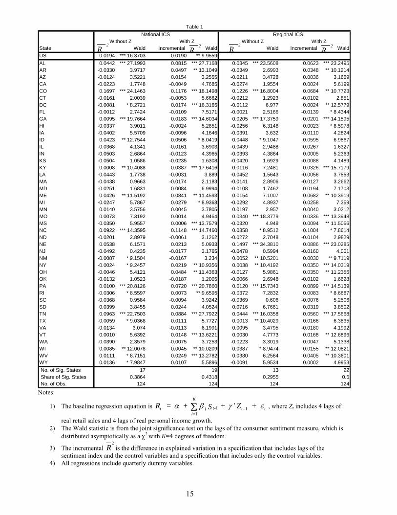
The impact of consumer sentiment on retail sales growth is shown in Table 1. This table

presents the adjusted R2 from the regressions with the national and regional ICS, as well as the

Wald statistic for the joint significance test on the lags of the consumer sentiment measure, which is

distributed asymptotically as a χ2 with K degrees of freedom. K represents the number of lags of the

sentiment variable, and therefore the number of linear restrictions in the test; in our case K = 4. The

table presents the significance tests without including the vector of control variables Z in columns

1, 2, and columns 5 and 6. We also conduct the joint significance tests conditioning on the vector

Z. In this case, the incremental adjusted R2 represents the difference in explained variation in a

specification that includes lags of the sentiment index and the control variables and a specification

that includes only the control variables.

The results with the national and regional ICS are very similar, although not the same states

present significant relationships in both cases. The consumer sentiment index predicts retail sales

growth in about 39 percent of the states in the sample when no additional variables are included. The

percentage of explained variation in retail sales growth, measured by the adjusted R2, in the states with

a significant relationship varies from 0 to about 17 percent, with an average of 2.8 percent using the

national ICS and an average of 4.6 percent using the regional ICS.9 The geographic pattern of the

significance results when using the national ICS can be observed in Figure 2, where we have also

outlined the ICS regions.

When additional control variables are included, the consumer sentiment/retail sales growth

relationship is significant in 19 out of the 44 sample states, when using the national ICS, and in 22

states, when using the regional ICS. The incremental variation explained by the lagged consumer

8

sentiment in the states with a significant relationship varies from 0 to about 12 percent, using the

national ICS, with an average of 4.6 percent; the incremental explained variation varies from 0 to

about 10 percent, with an average of 3.7 percent, when using the regional ICS.

[Table 1 about here]


The results with the national CCI are summarized in Table 2. With no additional control variables,

the consumer sentiment/retail sales relationship is significant in about 27 percent of the sample

states, and the adjusted R2 varies from 0 to about 15 percent, with an average of 3.5 percent among

the states with a significant relationship. When additional control variables are included, the

relationship is significant in about 43 percent of the sample states. The incremental adjusted R2

varies from 0 to about 12 percent, with an average of 4.3 percent among the states with a significant

relationship.


We learn from these tables that consumer sentiment lags predict retail sales growth in as

much as 39 percent of the states analyzed, when used as the only regressors, and in as much as half

of the sample states, when adding other control variables. The percentage of explained retail sales

growth variation, however, rarely exceeds 5 percent among the sample states. In contrast, about

14 percent of the variation in consumer expenditure growth is explained by consumer sentiment

lags in the results reported by Carroll et al. Nevertheless, the incremental variation, with respect to

including additional controls, often exceeds 2 percent, which is in line with the 3 percent of

incremental variation of consumer spending growth explained by consumer sentiment reported by

Carroll et al. These results indicate that, although the relationship between consumer sentiment and

state retail sales growth appears to be significant in many states, consumer sentiment has limited

predictive power for future changes of retail spending, as measured by the percentage of explained

9 Negative values of the adjusted R2 were set to 0 to compute the averages.

9

variation in the regression. Measures of consumer sentiment, however, contain additional

explanatory power aside from the information available from other indicators.

Regarding the national retail sales model, we find that the consumer sentiment/retail sales

growth relationship is significant in both the national ICS and the national CCI. The CCI, when

used without additional control variables, explains about 4 percent of the retail sales growth

variation, while the ICS explains only about 2 percent. The predictive power of the CCI over the

ICS is consistent with Bram and Ludvigson (1998). The incremental increase in adjusted R2 ,

when including additional control variables, is 1.9 percent with the ICS and 4.7 percent with the

CCI.

4. Discussion

The empirical results suggest that consumer sentiment measures are relatively poor

predictors of state-level retail sales growth. At the national level, we find that consumer sentiment

appears to perform as well as in the average state with a significant relationship between consumer

sentiment and retail sales growth. This raises two questions: (1) are the national results driven by a

few states with a highly significant relationship between sentiment and retail sales growth, and (2)

does the use of aggregated data mitigate large variations in state-level retail sales growth?

4.1 Are the national results driven by a few states?

To answer the first question, we conducted the following exercise. We ranked the

individual state regressions in decreasing order of adjusted R2, then iteratively subtracted the level

of that state’s retail sales from the national aggregate, re-computing the growth rate of national

retail sales. At each step, we ran the national regression using the new dependent variable and

tested again for the joint significance of the consumer sentiment measures. If the national results

are driven by the top significant states, then one would expect the significance of the sentiment

10

coefficients in the national regression to drop quickly once retail sales from the significant states

are subtracted out. Table 3 presents a summary of this exercise, listing, for each case of the state

regressions, the number of states that have to be removed before the national regression loses

significance. Each row in the table indicates a regression at the state level from which we ordered

the states in terms of the adjusted R2 coefficient.


Table 3 provides evidence that the impact of sentiment on national retail sales does not

appear to be the result of a strong relationship between sentiment and retail sales growth in only a

few states. Using the national or regional ICS as the sentiment measure in the state regressions, we

find that we have to remove 20 and 19 states, respectively, to render the national regression

insignificant (with the ICS as the dependent variable and no additional explanatory variables).

However, when including additional explanatory variables in the national and state regressions, we

have to remove only 6 states before the national regression loses significance. This indicates that

the predictive power of this sentiment measure when additional explanatory variables are included

in the national regression is somewhat less robust. In contrast, we find that the predictive power of

CCI is robust in the national regression also when including additional explanatory variables. In

the specification with no additional variables we have to remove 14 states before the national

regression loses significance. The CCI measure in the specification with additional variables

remains significant even when we iteratively subtract every state in the sample.

4.2 Does the use of national-level data mitigate large variations in state-level data?

With regards to the second question, it is possible that idiosyncratic state-level variation in

retail sales is sufficiently large to confound prediction of disaggregated retail sales but washes out

in aggregation. The sum of squared residuals for the national and state-level regressions can provide

insight into this scenario. It turns out that for each of the state-level specifications, with the

exception of Alabama, the sum of squared residuals for a state-level regression is equal or larger

11

than the sum of squared residuals for the corresponding national regression. Large variations in

retail sales growth at the state level appear to be mitigated by aggregating states to the national

level, thus providing a more predictable data series.

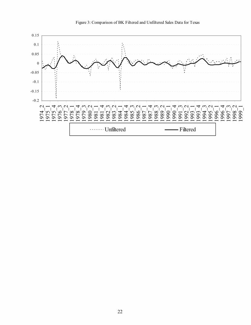
If these idiosyncratic state-level fluctuations in retail sales are indeed responsible for

confounding the state regressions, restricting our attention to the variations in retail sales that occur

at a business cycle frequency might increase the indices’ explanatory power. We accomplish this

by employing the Baxter-King bandpass filter (henceforth, BK filter) to the retail sales and

consumer sentiment data.11 The algorithm has the effect of filtering out fluctuations that occur

outside a pre-specified periodic band. Since we are interested in business cycle fluctuations, we

parameterize the filter using Baxter and King’s suggestion of filtering out fluctuations with

periodicity lower than eighteen months and greater than eight years. An example of the resulting

bandpassed series and the original retail sales data for Texas is plotted in Figure 3. Specifically,

note that the BK filter eliminates the high frequency noise in the retail sales series.


[Tables 4 and 5 about here]

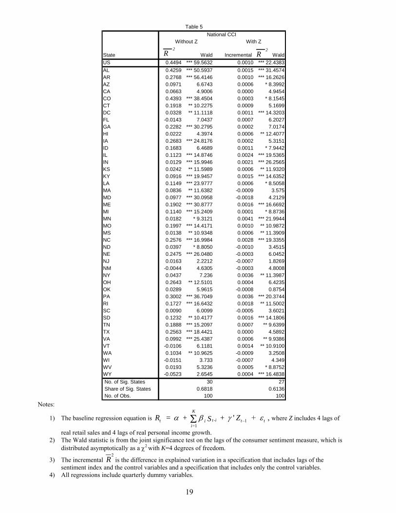
Using the BK-filtered data, we perform the same regressions from section 3. Results are

illustrated in Tables 4 and 5. We find that, sans high frequency noise, the explanatory power of

consumer sentiment increases considerably. In fact, the number of states in which lags of national

ICS enter significantly in the joint test, once the high frequency fluctuations are filtered out, jumps

from 17 to 30, and the average adjusted R2 equals 15.5 percent among these states. The number of

states in which lags of regional ICS enter significantly jumps from 13 to 30, with an average

adjusted R2 of 14.5 percent. The number of states in which lagged CCI enters significantly

increases from 12 to 30, with an average adjusted R2 of 16.6 percent. The national estimates are

significant in both the ICS and CCI cases. The adjusted R2 equals 33.4 percent using the ICS and

44.9 percent using the CCI. The average increment in explained variation when using additional

12

control variables, however, does not exceed 0.1 percent in any of the specifications, suggesting that

no additional information is provided by the consumer sentiment indices that is not contained in the

control variables.

This increase in explanatory power across states suggests that high-frequency fluctuations

do confound the assessment of consumer sentiment’s merit in evaluating regional economic

conditions. While these results validate in part the theory of employing consumer sentiment indices

to predict economic conditions, the practical value of the indices as forecasting instruments is

limited. Although the results imply that the business cycle component of the indices (that is,

fluctuations that occur with business cycle periodicity) are useful in forecasting the business cycle

component of retail sales, forecasting actual retail sales from actual consumer sentiment, however,

is problematic because filtering the data requires dropping observations at the end of sample as

well, not just at the beginning. Thus, the indices may provide some indication about the overall

state of the regional economy but little information about next month’s data releases.

5. Summary

In this paper we examine how well consumer sentiment predicts state-level retail sales

growth. The empirical results suggest that consumer sentiment measures are relatively weak

predictors of state-level retail sales growth. We find that, on average, consumer sentiment forecasts

retail sales growth for at least 27 percent of the 44 states we analyzed. In those states having a

significant sentiment/spending relationship the incremental explanatory power of including lagged

sentiment to the forecasting models averages about 4 percent.

We find that consumer sentiment predicts national-level retail sales growth. This, however,

raises the question of what may explain the difference in results between state and national

forecasting models. This study shows that aggregation at the national level mitigates random state-

level variations in retail sales growth. However, while data aggregation reduces state-level

11 See Baxter and King (1999) for details about this filter.

13

variations in retail sales growth, our analysis also revealed that the significant sentiment and

spending relationship using national retail sales is not driven by a strong sentiment/spending

relationship in only a few states. Focusing the investigation on fluctuations at the business cycle

frequency reveals a significant sentiment/spending relationship in a greater number of states. The

findings here reveal that, while consumer sentiment may help assess the general state of the

national economy, it may not be an important factor in forecasting regional economic growth.

14

References Allenby, Greg M., Jen, Lichung, and Leone, Robert P. “Economic Trends and Being Trendy: The Influence of Consumer Confidence on Retail Fashion Sales.” Journal of Business and Economic Statistics, January 1996, 14(1), pp. 103-11. Batchelor, Roy, and Dua, Pami. “Improving Macro-economic Forecasts: The Role of Consumer Confidence.” International Journal of Forecasting, March 1998, 14(1), pp. 71-81. Baxter, Marianne, and King, Robert G. “Measuring Business Cycles: Approximate Band-Pass Filters for Economic Time Series.” Review of Economics and Statistics, November 1999, 81(4), pp. 575-93. Bram, Jason, and Ludvigson, Sydney. “Does Consumer Confidence Forecast Household Expenditure? A Sentiment Index Horse Race.” Federal Reserve Bank of New York Economic Policy Review, June 1998, 4(2), pp. 59-78. Carroll, Christopher D., Fuhrer, Jeffrey C., and Wilcox, David W. “Does Consumer Sentiment Forecast Household Spending? If so, why?” American Economic Review, December 1994, 84(5), pp. 1397-1408. Howrey, E. Philip. “The Predictive Power of the Index of Consumer Sentiment.” Brookings Papers on Economic Activity, 2001, 0(1), pp. 175-207. Leeper, Eric M. “Consumer Attitudes: King for a Day.” Federal Reserve Bank of Atlanta Economic Review, July-August 1992, 77(4), pp. 1-15. Matsusaka, John G., and Sbordone, Argia M. “Consumer Confidence and Economic Fluctuations.” Economic Inquiry, April 1995, 33(2), pp. 296-318. Owyang, Michael T., Piger, Jeremy and Wall, Howard J. “Business Cycle Phases in U.S. States.” Federal Reserve Bank of St. Louis Working Paper 2003-011E, 2004. Piger, Jeremy, “Consumer Confidence Surveys. Do They Boost Forecasters’ Confidence?” The Regional Economist, April 2003, pp. 10-11. Rodgers, James D., and Temple, Judy A. “Sales Taxes, Income Taxes, and Other Non-Property Tax Revenues.” in Management Policies in Local Government Finance, Municipal Management Series, Washington, D.C.: International City/County Management Association for the ICMA University, 1996, 4th edition, pp. 229-57

15

State Wald Incremental Wald Wald Incremental WaldUS 0.0194 *** 16.3703 0.0190 ** 9.9559AL 0.0442 *** 27.1993 0.0815 *** 27.7168 0.0345 *** 23.5608 0.0623 *** 23.2495AR -0.0330 3.9717 0.0497 ** 13.1049 -0.0349 2.6993 0.0348 ** 10.1214AZ -0.0124 3.5221 0.0154 3.2555 -0.0211 3.4728 0.0036 3.1669CA -0.0223 1.7748 -0.0049 4.7685 -0.0274 1.9554 0.0024 5.6199CO 0.1697 *** 24.1463 0.1176 *** 18.1498 0.1226 *** 16.8004 0.0684 ** 10.7723CT -0.0161 2.0039 -0.0053 5.6662 -0.0212 1.2923 -0.0102 2.851DC -0.0081 * 8.2721 0.0174 *** 16.3165 -0.0112 6.977 0.0024 ** 12.5779FL -0.0012 2.7424 -0.0109 7.5171 -0.0021 2.5166 -0.0139 * 8.4344GA 0.0095 *** 19.7664 0.0183 *** 14.6034 0.0205 *** 17.3759 0.0201 *** 14.1595HI -0.0337 3.9011 -0.0024 5.2851 -0.0256 6.3148 0.0023 * 8.5978IA -0.0402 5.5709 -0.0096 4.1646 -0.0391 3.632 -0.0110 4.2824ID 0.0423 ** 12.7544 0.0506 * 8.0419 0.0448 * 9.1047 0.0595 6.9867IL -0.0368 4.1341 -0.0161 3.6903 -0.0439 2.9488 -0.0267 1.6327IN -0.0503 2.6864 -0.0123 4.3965 -0.0393 4.3864 0.0005 5.2363KS -0.0504 1.0586 -0.0235 1.6308 -0.0420 1.6929 -0.0088 4.1489KY -0.0008 ** 10.4088 0.0387 *** 17.6416 -0.0116 7.2481 0.0326 *** 15.7179LA -0.0443 1.7738 -0.0031 3.889 -0.0452 1.5643 -0.0056 3.7553MA -0.0438 0.9663 -0.0174 2.1183 -0.0141 2.8906 -0.0127 3.2662MD -0.0251 1.6831 0.0084 6.9994 -0.0108 1.7462 0.0194 7.1703ME 0.0426 ** 11.5192 0.0841 ** 11.4593 0.0154 7.1007 0.0682 ** 10.3919MI -0.0247 5.7867 0.0279 * 8.9368 -0.0292 4.8937 0.0258 7.359MN 0.0140 3.5756 0.0045 3.7805 0.0197 2.957 0.0040 3.0212MO 0.0073 7.3192 0.0014 4.9464 0.0340 *** 18.3779 0.0336 *** 13.3948MS -0.0350 5.9557 0.0006 *** 13.7579 -0.0320 4.948 0.0094 ** 11.5056NC 0.0922 *** 14.3595 0.1148 *** 14.7460 0.0858 * 8.9512 0.1004 * 7.8614ND -0.0201 2.8979 -0.0061 3.1262 -0.0272 2.7048 -0.0104 2.9829NE 0.0538 6.1571 0.0213 5.0933 0.1497 *** 34.3810 0.0886 *** 23.0285NJ -0.0492 0.4235 -0.0177 3.1765 -0.0478 0.5994 -0.0160 4.001NM -0.0087 * 9.1504 -0.0167 3.234 0.0052 ** 10.5201 0.0030 ** 9.7119NY -0.0024 * 9.2457 0.0219 ** 10.9356 0.0038 ** 10.4192 0.0350 *** 14.0319OH -0.0046 5.4121 0.0484 ** 11.4363 -0.0127 5.9861 0.0350 ** 11.2356OK -0.0132 1.0523 -0.0187 1.2005 -0.0066 2.6948 -0.0102 1.6628PA 0.0100 *** 20.8126 0.0720 *** 20.7860 0.0120 *** 15.7343 0.0899 *** 14.5139RI -0.0306 * 8.5597 0.0073 ** 9.6595 -0.0372 7.2832 0.0083 * 8.6687SC -0.0368 0.9584 -0.0094 3.9242 -0.0369 0.606 -0.0076 5.2506SD 0.0399 3.8455 0.0244 4.0524 0.0716 6.7661 0.0319 3.8502TN 0.0963 *** 22.7503 0.0884 *** 27.7922 0.0444 *** 16.0358 0.0560 *** 17.5668TX -0.0059 * 9.0368 0.0111 5.7727 0.0013 ** 10.4029 0.0166 6.3835VA -0.0134 3.074 -0.0113 6.1991 0.0095 3.4795 -0.0180 4.1992VT 0.0010 5.6392 0.0148 *** 13.6221 0.0030 4.7773 0.0168 ** 12.6896WA -0.0390 2.3579 -0.0075 3.7253 -0.0223 3.3019 0.0047 5.1338WI 0.0085 ** 12.0078 0.0045 ** 10.0209 0.0387 * 8.9474 0.0155 ** 12.0821WV 0.0111 * 8.7151 0.0249 *** 13.2782 0.0380 6.2564 0.0405 ** 10.3601WY 0.0136 * 7.9847 0.0107 5.5896 -0.0091 5.9534 0.0002 4.9953 No. of Sig. States 17 19 13 22 Share of Sig. States 0.3864 0.4318 0.2955 0.5 No. of Obs. 124 124 124 124

Table 1National ICS Regional ICS

Without Z With Z Without Z With Z2

R2

R2R

2R

Notes:

1) The baseline regression equation is 11

' + K

t-it t tii=

R = + + ZSα γ εβ −Σ , where Zt includes 4 lags of

real retail sales and 4 lags of real personal income growth. 2) The Wald statistic is from the joint significance test on the lags of the consumer sentiment measure, which is

distributed asymptotically as a χ2 with K=4 degrees of freedom.

3) The incremental 2

R is the difference in explained variation in a specification that includes lags of the sentiment index and the control variables and a specification that includes only the control variables.

4) All regressions include quarterly dummy variables.

16

State Wald Incremental WaldUS 0.0395 *** 16.2407 0.0470 ** 9.5723AL 0.0267 *** 29.5784 0.0423 *** 18.1061AR -0.0299 3.1322 0.0445 *** 15.3454AZ 0.0163 ** 10.6010 0.0583 * 9.0056CA -0.0185 5.0044 -0.0020 4.942CO 0.1512 *** 25.8783 0.0941 *** 20.9290CT -0.0308 0.2611 -0.0179 1.5915DC -0.0195 5.4149 0.0109 * 8.6949FL -0.0079 3.2429 -0.0016 6.5437GA 0.0008 *** 23.6877 0.0407 *** 23.0608HI -0.0195 5.813 0.0242 * 8.2153IA -0.0534 0.6954 -0.0125 2.2808ID 0.0206 *** 15.3374 0.0466 ** 11.9457IL -0.0308 2.7776 0.0040 6.4904IN -0.0551 1.0435 -0.0200 3.0961KS -0.0327 5.9747 -0.0031 6.063KY -0.0176 6.4156 0.0297 *** 13.5088LA -0.0311 4.5513 -0.0097 3.6195MA -0.0452 5.3728 0.0071 *** 15.4617MD -0.0256 0.9191 -0.0015 1.7196ME 0.0406 *** 16.0393 0.0792 ** 12.2705MI -0.0165 5.7469 0.0291 ** 9.9917MN 0.0087 3.3834 -0.0030 2.7751MO 0.0016 ** 9.8358 0.0050 6.2007MS -0.0390 7.235 0.0008 ** 13.1303NC 0.0963 ** 10.7041 0.1182 *** 16.2520ND -0.0196 3.4301 -0.0046 4.0016NE 0.0185 5.1149 0.0067 4.3593NJ -0.0348 1.7404 -0.0159 3.0367NM -0.0161 4.2911 -0.0236 1.202NY -0.0285 2.0339 -0.0143 2.689OH -0.0141 1.5769 0.0514 * 8.6690OK -0.0214 0.5755 -0.0238 0.8261PA 0.0064 *** 19.0759 0.0697 *** 13.6032RI -0.0101 5.3615 -0.0188 3.2067SC -0.0378 0.6484 -0.0093 3.4403SD 0.0032 3.0572 0.0309 4.8005TN -0.0022 5.3644 0.0260 *** 16.2701TX 0.0040 ** 10.2062 0.0015 6.4641VA -0.0213 1.1928 -0.0092 3.8202VT 0.0007 * 8.2720 0.0200 *** 16.4255WA -0.0456 0.5312 -0.0097 3.1324WI -0.0133 4.2399 0.0049 4.6503WV 0.0507 *** 14.1404 0.0233 * 9.1675WY -0.0007 5.4429 0.0078 4.4185 No. of Sig. States 12 19 Share of Sig. States 0.2727 0.4318 No. of Obs. 124 124

National CCI Without Z With Z

Table 2

2R 2

R

Notes:


' + K

t-it t tii=

R = + + ZSα γ εβ −Σ , where Z includes 4 lags of






17

Table 3: National Model: Iterative Subtraction of Top Significant States

States Regression Subtracted States*Nat. ICS 20Nat. ICS with Z 6Reg. ICS 19Reg. ICS with Z 6Nat. CCI 14Nat. CCI with Z 43

* Number of states that have to be removed from the calculation of national retail sales before lags of consumer sentiment lose

significance in the national regression.

18

State Wald Incremental Wald Wald Incremental WaldUS 0.3337 *** 45.2977 0.0006 ** 13.0699AL 0.4461 *** 67.7667 0.0020 *** 30.0992 0.4479 *** 62.8791 0.0018 *** 30.7239AR 0.2375 *** 37.9923 0.0003 4.5625 0.1596 *** 24.6486 0.0010 * 8.1242AZ 0.0171 4.9411 0.0005 6.7998 0.0136 6.6199 0.0001 5.35CA 0.1503 7.0782 0.0016 *** 13.5792 0.1571 ** 11.9313 0.0024 ** 12.1052CO 0.3463 *** 26.7764 0.0004 ** 10.9229 0.2763 *** 25.3171 0.0001 * 8.7513CT 0.1705 ** 9.6350 0.0013 *** 16.2784 0.0737 6.6263 0.0016 *** 16.6780DC 0.0098 *** 14.2995 0.0014 ** 11.4549 -0.0229 ** 10.1608 0.0014 ** 12.0484FL -0.0316 3.6356 0.0059 *** 13.9820 0.0433 2.8036 0.0054 ** 10.5561GA 0.1717 *** 17.3047 0.0000 * 8.5662 0.1321 *** 14.0626 -0.0003 6.4041HI 0.0018 4.5091 -0.0003 6.2346 -0.0060 5.0868 -0.0003 * 8.4027IA 0.1378 ** 11.4569 -0.0007 2.0571 0.1582 *** 14.8744 -0.0007 2.5608ID 0.1543 * 8.5366 -0.0001 1.9097 0.1070 * 8.0150 -0.0002 1.7068IL 0.1326 *** 16.8109 0.0000 6.389 0.1734 *** 21.3654 0.0002 *** 13.3735IN 0.0922 *** 17.0641 0.0018 *** 26.6683 0.1911 *** 20.8963 0.0018 *** 27.0175KS 0.0035 *** 16.0447 -0.0006 2.1206 0.0258 *** 21.0589 -0.0007 2.1018KY 0.0038 ** 11.3802 -0.0007 5.0612 0.0191 *** 13.5870 -0.0009 3.5954LA 0.0318 ** 11.9219 -0.0004 5.2552 0.0570 *** 17.8756 -0.0004 5.8511MA 0.1506 *** 14.1654 0.0010 7.2287 0.1792 *** 21.6907 0.0001 4.3149MD -0.0151 4.8609 -0.0023 3.9027 -0.0007 3.5998 -0.0024 3.7002ME 0.2946 *** 33.6198 0.0023 *** 20.5371 0.2490 *** 26.9085 0.0025 *** 23.3702MI 0.1019 * 8.2941 -0.0006 4.5142 0.1179 ** 12.2485 0.0001 7.228MN 0.0039 6.7072 -0.0011 3.8667 0.0593 ** 12.2624 -0.0011 4.0118MO 0.1763 ** 12.4560 0.0002 3.2518 0.2020 *** 16.4107 0.0003 4.3417MS 0.0443 ** 12.7706 0.0017 * 8.5699 0.1088 *** 16.4688 0.0021 ** 10.5523NC 0.2089 *** 14.2964 0.0038 *** 28.6966 0.1205 ** 9.9927 0.0034 *** 31.5400ND 0.0253 4.584 -0.0006 6.3773 -0.0142 3.138 -0.0006 6.2748NE 0.0579 6.3143 0.0005 ** 9.9377 0.0818 * 8.6343 0.0007 ** 11.9757NJ -0.0144 2.7231 -0.0010 1.4506 -0.0443 1.0448 -0.0011 0.803NM 0.0663 ** 12.0026 0.0003 * 8.2425 0.0365 ** 11.1883 -0.0001 6.6917NY 0.1601 *** 18.7195 0.0057 *** 13.6368 0.1859 *** 19.2699 0.0080 *** 19.1539OH 0.2901 *** 21.4710 0.0010 7.0026 0.3099 *** 22.8270 0.0005 6.6274OK 0.0019 ** 9.5713 -0.0005 3.7905 0.0001 * 8.1625 -0.0007 1.8234PA 0.3371 *** 42.8525 0.0022 *** 13.7554 0.3399 *** 46.7987 0.0028 *** 15.4966RI 0.1539 ** 11.9046 0.0008 ** 9.7213 0.1439 ** 12.3703 0.0006 ** 11.2415SC 0.0250 5.5716 0.0005 ** 10.4328 0.0180 5.219 -0.0005 5.4714SD 0.0466 ** 10.0845 0.0004 * 8.8026 0.0208 * 8.1881 -0.0001 5.4646TN 0.3684 *** 43.2376 0.0007 ** 11.4612 0.3287 *** 31.8020 0.0007 *** 15.8775TX 0.0363 *** 19.5994 -0.0006 0.3641 0.0639 *** 26.0904 -0.0006 0.4355VA 0.2915 *** 52.5277 0.0013 *** 13.5755 0.2034 *** 44.2381 0.0007 ** 9.9447VT 0.0189 6.121 0.0023 *** 17.4817 0.0147 6.0123 0.0018 *** 16.2494WA 0.0693 7.6779 -0.0002 6.0483 0.0115 3.7351 -0.0004 6.3913WI -0.0002 * 9.3039 0.0004 * 8.3219 0.0189 ** 13.2683 0.0005 * 8.6497WV -0.0168 3.1777 0.0011 *** 19.1226 -0.0355 1.7039 0.0006 *** 13.8610WY -0.0591 1.3146 -0.0003 ** 11.7378 -0.057 1.1186 -0.0004 ** 9.6988No. of Sig. States 30 24 32 23 Share of Sig. States 0.6818 0.5455 0.7273 0.5227 No. of Obs. 100 100 100 100

Without Z With Z

Regional ICSTable 4

Without Z With Z

National ICS

2R 2

R2R

2R

Notes:


' + K

t-it t tii=



distributed asymptotically as a χ2 with K =4 degrees of freedom.




19

State Wald Incremental WaldUS 0.4494 *** 59.5632 0.0010 *** 22.4383AL 0.4259 *** 50.5937 0.0015 *** 31.4574AR 0.2768 *** 56.4146 0.0010 *** 16.2626AZ 0.0971 6.6743 0.0006 * 8.3992CA 0.0663 4.9006 0.0000 4.9454CO 0.4393 *** 38.4504 0.0003 * 8.1545CT 0.1918 ** 10.2275 0.0009 5.1699DC 0.0328 ** 11.1118 0.0011 *** 14.3203FL -0.0143 7.0437 0.0007 6.2027GA 0.2282 *** 30.2795 0.0002 7.0174HI 0.0222 4.3974 0.0006 ** 12.4077IA 0.2683 *** 24.8176 0.0002 5.3151ID 0.1683 6.4689 0.0011 * 7.9442IL 0.1123 *** 14.8746 0.0024 *** 19.5365IN 0.0129 *** 15.9946 0.0021 *** 26.2565KS 0.0242 ** 11.5989 0.0006 ** 11.9320KY 0.0916 *** 19.9457 0.0015 *** 14.6352LA 0.1149 *** 23.9777 0.0006 * 8.5058MA 0.0836 ** 11.6382 -0.0009 3.575MD 0.0977 *** 30.0958 -0.0018 4.2129ME 0.1902 *** 30.8777 0.0016 *** 16.6692MI 0.1140 *** 15.2409 0.0001 * 8.8736MN 0.0182 * 9.3121 0.0041 *** 21.9944MO 0.1997 *** 14.4171 0.0010 ** 10.9872MS 0.0138 ** 10.9348 0.0006 ** 11.3909NC 0.2576 *** 16.9984 0.0028 *** 19.3355ND 0.0397 * 8.8050 -0.0010 3.4515NE 0.2475 *** 26.0480 -0.0003 6.0452NJ 0.0163 2.2212 -0.0007 1.8269NM -0.0044 4.6305 -0.0003 4.8008NY 0.0437 7.236 0.0036 ** 11.3987OH 0.2643 ** 12.5101 0.0004 6.4235OK 0.0289 5.9615 -0.0008 0.8754PA 0.3002 *** 36.7049 0.0036 *** 20.3744RI 0.1727 *** 16.6432 0.0018 ** 11.5002SC 0.0090 6.0099 -0.0005 3.6021SD 0.1232 ** 10.4177 0.0016 *** 14.1806TN 0.1888 *** 15.2097 0.0007 ** 9.6399TX 0.2563 *** 18.4421 0.0000 4.5892VA 0.0992 *** 25.4387 0.0006 ** 9.9386VT -0.0106 6.1181 0.0014 ** 10.9100WA 0.1034 ** 10.9625 -0.0009 3.2508WI -0.0151 3.733 -0.0007 4.349WV 0.0193 5.3236 0.0005 * 8.8752WY -0.0523 2.6545 0.0004 *** 16.4838 No. of Sig. States 30 27 Share of Sig. States 0.6818 0.6136 No. of Obs. 100 100

National CCI Without Z With Z

Table 5

2R 2

R

Notes:


' + K

t-it t tii=







20

Figure 1: Consumer Sentiment and Personal Consumption Expenditures

40

60

80

100

120

140

1970

_1

1971

_2

1972

_3

1973

_4

1975

_1

1976

_2

1977

_3

1978

_4

1980

_1

1981

_2

1982

_3

1983

_4

1985

_1

1986

_2

1987

_3

1988

_4

1990

_1

1991

_2

1992

_3

1993

_4

1995

_1

1996

_2

1997

_3

1998

_4

2000

_1

2001

_2

ICS,

CC

I

-3.00

-2.00

-1.00

0.00

1.00

2.00

3.00

Log

Diff

eren

ce o

f PC

E

cci ics Diff_log_PCE

21

Figure 2: Significance Levels by Region

22

Figure 3: Comparison of BK Filtered and Unfiltered Sales Data for Texas

-0.2

-0.15

-0.1

-0.05

0

0.05

0.1

0.15

1974

_219

75_1

1975

_419

76_3

1977

_219

78_1

1978

_419

79_3

1980

_219

81_1

1981

_419

82_3

1983

_219

84_1

1984

_419

85_3

1986

_219

87_1

1987

_419

88_3

1989

_219

90_1

1990

_419

91_3

1992

_219

93_1

1993

_419

94_3

1995

_219

96_1

1996

_419

97_3

1998

_219

99_1

Unfiltered Filtered

Date post:	11-Feb-2022
Category:	Documents
Upload:	others
View:	3 times
Download:	0 times

Does Consumer Sentiment Predict Regional Consumption?

Documents