Federal Reserve Bank of MinneapolisResearch Department Staff Report 363

June 2005

Does Income Inequality Lead to Consumption Equality?Evidence and Theory

Dirk Krueger∗

Goethe University Frankfurt,University of Pennsylvania,National Bureau of Economic Research,and Centre for Economic Policy Research

Fabrizio Perri∗

Federal Reserve Bank of Minneapolis,New York University,National Bureau of Economic Research,and Centre for Economic Policy Research

ABSTRACT

Using data from the Consumer Expenditure Survey, we first document that the recent increase inincome inequality in the United States has not been accompanied by a corresponding rise in con-sumption inequality. Much of this divergence is due to different trends in within-group inequality,which has increased significantly for income but little for consumption. We then develop a simpleframework that allows us to analytically characterize how within-group income inequality affectsconsumption inequality in a world in which agents can trade a full set of contingent consumptionclaims, subject to endogenous constraints emanating from the limited enforcement of intertemporalcontracts (as in Kehoe and Levine, 1993). Finally, we quantitatively evaluate, in the context ofa calibrated general equilibrium production economy, whether this setup, or alternatively a stan-dard incomplete markets model (as in Aiyagari, 1994), can account for the documented stylizedconsumption inequality facts from the U.S. data.

∗We thank the editor, Fabrizio Zilibotti, three anonymous referees, and seminar participants at numerousinstitutions and conferences for their many and very helpful comments. Many thanks also to Harris Dellasand Pierre-Olivier Gourinchas for their thoughtful discussions and to Carlos Serrano and Cristobal Huneeusfor outstanding research assistance. Krueger gratefully acknowledges financial support from the NationalScience Foundation under grant SES-0004376. The views expressed herein are those of the authors and notnecessarily those of the Federal Reserve Bank of Minneapolis or the Federal Reserve System.

1 Introduction

The sharp increase in earnings and income inequality for the United States in the last 25 years

is a well-documented fact. Many authors have found that the dispersions of U.S. household

earnings and incomes have a strong upward trend, attributable to increases in the dispersion of

the permanent component of income as well as to an increase in the volatility of the transitory

component of income.1 If one is interested in the welfare impact of these changes, however, the

distribution of current income might not be a sufficient statistic. Since a significant fraction of

variations of income appear to be due to variations in its transitory component, current income

may not be the appropriate measure of lifetime resources available to agents; and thus the dis-

tribution of current income might not be a good measure of how economic welfare is allocated

among households in the United States.2 Moreover, the same change in current or permanent

income inequality might have a very different impact on the welfare distribution, depending on

the structure of credit and insurance markets available to agents for smoothing income fluctua-

tions. For these reasons, several authors have moved beyond income and earnings as indicators

of well-being and have studied the distribution of individual or household consumption. Con-

tributors include Cutler and Katz (1991a,b), Johnson and Shipp (1991), Johnson and Smeeding

(1998), Mayer and Jencks (1993), Slesnick (1993, 2001), Deaton and Paxson (1994), Dynarski

and Gruber (1997), Blundell and Preston (1998), and Krueger and Perri (2004).

Our paper follows this line of research and aims at making three contributions, one empir-

ical, one theoretical, and one quantitative in nature. On the empirical side it investigates how

the cross-sectional income and consumption distribution in the United States developed over

the period 1980—2003. Using data from the Consumer Expenditure Survey, the paper extends

and complements the studies mentioned above. Our main finding is that despite the surge in

income inequality in the United States in the last quarter century, consumption inequality has

increased only moderately. In particular, income inequality has increased substantially both

between and within groups of households with the same characteristics (such as education, sex,

and race), but even though between-group consumption inequality has tracked between-group

1See, e.g., Gottschalk and Moffitt (1994), Gottschalk and Smeeding (1997), or Katz and Autor (1999) forrecent surveys of these empirical findings.

2Blundell and Preston (1998) provide theoretical conditions under which the cross-sectional distribution ofcurrent consumption is a sufficient statistic for the cross-sectional distribution of welfare.

1

income inequality quite closely, within-group consumption inequality has increased much less

than within-group income inequality.

Second, we propose a theoretical explanation for these stylized facts. Our hypothesis is that

an increase in the volatility of idiosyncratic labor income (which we identify as the increase

in within-group inequality) not only has been an important factor in the increase in income

inequality, but also has caused a change in the development of financial markets, allowing indi-

vidual households to better insure against these (now bigger) idiosyncratic income fluctuations.

We present a simple model with endogenous debt constraints (henceforth referred to as the debt

constraint markets (DCM) model), building on earlier work by Alvarez and Jermann (2000),

Kehoe and Levine (1993, 2001), and Kocherlakota (1996), that allows us to analytically charac-

terize the relationship between within-group income and consumption inequality. In the model

agents enter risk-sharing contracts, but at any point in time have the option to renege on their

obligations, at the cost of losing their assets and being excluded from future risk sharing. Our

main result is that an increase in the volatility of income, keeping the persistence of the income

process constant, always leads to a smaller increase in consumption inequality within the group

that shares income risk, unless there is no capital income in the economy. The nondegenerate

range of income dispersion is such that an increase in income volatility leads to a decline in

consumption inequality. Intuitively, we know that higher income volatility increases the value

of risk-sharing opportunities and therefore reduces the incentives to default. As a consequence,

more risk sharing is possible and the consumption distribution fans out less than the income dis-

tribution (and may even “fan in”). This model captures, in a simple and analytically tractable

way, the idea that the structure of the credit markets in an economy is endogenous and that,

in response to higher income volatility, credit markets have more value and thus will tend to

deepen.3

Finally, we assess whether an extension of this simple model is quantitatively consistent with

the stylized facts established in the empirical section of the paper. We develop a production

economy with capital and a large number of agents that face a stochastic labor income process.

3The endogenous response of credit markets to income risk has interesting policy implications. In Kruegerand Perri (1999) we show that in the DCM model public insurance (unemployment insurance, progressive taxes,etc.) may crowd out private insurance, possibly more than one-for-one. Empirical studies by Cutler and Gruber(1996) and Albarran and Attanasio (2003) find a sizeable crowding-out effect of public insurance programs.

2

We choose this income process to match the level and trend of income inequality, both between

and within different groups. In particular, we also allow for changes in income inequality that

are not due to changes in income volatility. The extent to which agents can borrow to insulate

consumption from idiosyncratic income fluctuations is derived endogenously. It is a function

of the volatility of the stochastic income process, which, as before in the simple model, affects

the incentives to repay loans by determining how valuable future access to credit markets is.

Our model, for a given time series of cross-sectional income distributions, produces a time series

of cross-sectional between- and within-group consumption distributions. We also evaluate the

quantitative implications for within- and between-group consumption inequality of a standard

incomplete markets model (henceforth referred to as the SIM model) along the lines of Aiyagari

(1994). We find that the DCM model slightly understates the increase in consumption inequality

and the SIM model somewhat overstates that increase, relative to the data.

The paper is organized as follows. In Section 2 we document our main stylized facts. Section

3 presents the simple model, and Section 4 lays out the economy we use for the quantitative

analysis. Section 5 describes our quantitative experiment and parameter choices, and Section

6 presents and discusses the results. Section 7 concludes. Appendix A contains more details

about the data and Appendix B more details about computational issues.

2 Trends in Income and Consumption Inequality

In this section we document how income and consumption inequality have evolved in the United

States during the last 25 years. For this purpose we use the Consumer Expenditure (CE)

Interview Survey, which is the only micro-level data set for the United States that reports

comprehensive measures of consumption expenditures and earnings for a repeated large cross

section of households.4

2.1 The Consumer Expenditure Survey

The CE Interview Survey is a rotating panel of households that are selected to be representative

of the U.S. population. It started in 1960, but continuous data are available only from the

4The Panel Study of Income Dynamics (PSID) reports both income and consumption data. The consumptiondata, however, contain only food consumption and therefore are of limited use for our analysis.

3

first quarter of 1980 until the first quarter of 2004. Each quarter the survey contains detailed

information on quarterly consumption expenditures for all households interviewed during that

quarter. After a first preliminary interview, each household is interviewed for a maximum of four

consecutive times. In the second and fifth interviews, household members are asked questions

about earnings, other sources of income, hours worked, and taxes paid for the past year.

2.2 Income and Consumption

Our measure of income is meant to capture all sources of household revenues that are exogenous

(to a large extent) to the consumption and saving decisions of households (which are endogenous

in our models). Therefore we define income as labor earnings after taxes plus transfers (from now

on, LEA+ income). We measure after-tax labor earnings as the sum of wages and salaries of all

household members, plus a fixed fraction of self-employment farm and nonfarm income,5 minus

reported federal, state, and local taxes (net of refunds) and Social Security contributions. We

then add reported government transfers (unemployment insurance, food stamps, and welfare).

Our measure of consumption is meant to capture the flow of consumption services that

accrue to a household in a given period. For nondurable or small semidurable goods as well as

services, expenditures are a good approximation for that flow. For large durable goods such as

cars and houses, the relation between current expenditures and consumption service flows is less

direct. Thus we impute service flows from the (value of the) stock of durables of a household.

Our measure of service flows from housing is the rent paid by the households who indeed rent

their home and the self-reported (by the CE respondent) hypothetical rent by the households

who own. Our measure of service flows of cars is a fixed fraction (1/32) of the value of the

stock of vehicles owned by the household. Since we do not have direct information on the

value of the stock of cars, we follow closely the procedure used by Cutler and Katz (1991a) and

use information from households who currently purchase vehicles (and for which we therefore

observe the value of the purchase) to impute the value of the stock of vehicles for all households.

Our benchmark measure of a household’s consumption is then the sum of expenditures on

nondurables, services, and small durables (such as household equipment), plus imputed services

from housing and vehicles. Each expenditure component is deflated by expenditure-specific,

5The exact fraction is 0.864 and is taken from Díaz-Giménez, Quadrini, and Ríos-Rull (1996).

4

quarter-specific consumer price indexes (CPIs). From now on we label this benchmark measure

ND+ consumption.6

As we are interested in the distribution of resources per capita, before computing inequality

measures we divide household income and consumption by the number of adult equivalents in

the household using the census equivalence scale (see Dalaker and Naifeh, 1998).

2.3 Sample Selection

Our objective is to characterize the link between labor income and consumption inequality.

Therefore we want to select a benchmark sample of households for which we have reliable data

for both labor income and consumption for the same time interval. To do so we restrict our

sample to households that are complete income respondents and interviewed four times.7 For

these households, income measured in the fifth interview and the sum of consumption figures

reported in the second through the fifth interviews are our measures of their yearly income

and consumption. For comparability with previous inequality studies, we performed additional

sample selections, such as excluding elderly households, rural households, and households whose

reference person reports an implausibly low real wage.8

In Table A2 in the appendix we report the benchmark sample sizes for every year in the

period 1980—2003, along with weighted averages for income and consumption. Note that the

data display no growth of expenditures on nondurables over time, as Slesnick (2001) already

highlights. This is puzzling since aggregate nondurable consumption expenditures from the Na-

tional Income and Product Accounts (NIPA) show significant growth (see again Slesnick, 2001).

This might be a signal for growing underreporting of nondurable consumption expenditures in

the CE. Also note, however, that ND+ consumption includes services from durables which, on

average, are almost as large as expenditures on nondurables (see again Table A2) and display

a growth trend over time that matches up better with NIPA data. So if underreporting of

consumption exists, it is likely to be less severe for our benchmark ND+ consumption measure

than for the more commonly used nondurable consumption expenditures.

6 In Appendix A we provide a detailed description of all the items included in our consumption measures andof our imputation and deflation procedures.

7The CE classifies as incomplete income respondents those households who report zero income for all the majorincome categories, suggesting nonreliability of their earning figures (see also Nelson, 1994).

8See Appendix A for a precise list of our sample restrictions.

5

2.4 Inequality Trends

Figure 1 displays the trend for four commonly used measures of cross-sectional inequality, com-

puted on the benchmark sample and on the measures of income and consumption described

above. All measures are computed using CE population weights. We report the Gini coeffi-

cient, the variance of the logs, and the 90/10 and 50/10 ratios. In each panel the dashed line

represents inequality in LEA+ income and the solid line represents inequality in ND+ consump-

tion. Finally the thin dash-dotted lines are standard errors of the inequality measures, which

we computed by performing a bootstrap procedure with 100 repetitions.

Figure 1 confirms the well-known fact that labor income inequality in the United States has

increased significantly in the last quarter century: the Gini index has risen from around 0.3 to

around 0.37, and the variance of the logs displays an increase of more than 20%. The 90/10

ratio for income surges from around 4.2 to over 6, suggesting a large divergence between the two

tails of the income distribution over time. Finally the 50/10 ratio displays an increase from 2.2

to about 2.7, revealing that households in the bottom tail of the income distribution have lost

ground relative to the median.9

The figure also presents our main empirical finding, namely that the increase in consumption

inequality has been much less marked;10 the increase has been from 0.23 to 0.26 for the Gini

and about 5% in the variance of logs. The 90/10 ratio has increased from 2.9 to around 3.4,

suggesting a much more moderate fanning out of the consumption distribution.11 Finally, the

50/10 ratio increases only from about 1.7 to 1.9, suggesting that in terms of consumption,

households in the bottom part of the distribution have lost less ground relative to the median.12

Note that our income definition includes government taxes and transfers, so that changes

in government income redistribution policies cannot be responsible for the divergence between

the two series. Although the evolution of consumption inequality has been studied less than

9Increases of similar magnitude are found in other cross-sectional data sets. Krueger and Perri (2004) comparethe increase in wage inequality using CE data with that obtained by using PSID data (from Heathcote et al.,2004) and the increase measured by using the Current Population Survey (CPS) data (from Katz and Autor,1999) and find that, for the same sample selection, the magnitude of the increase is very similar. This suggeststhat the quality of the CE earnings/wage data is comparable to those of other cross-sectional data sets.10Pendakur (1998) finds similar results for Canada for 1978—1992 and his preferred measure of consumption.11One nice property of the 90/10 ratios is that they are not sensitive to changes in top-coding thresholds. The

divergence of the 90/10 ratios in income and consumption thus suggests that changes in top-coding thresholdsplay no important role in explaining the measured divergence in inequality.12These findings are consistent with those of Slesnick (2001), who found that poverty rates for income increased

from 11.1% in 1973 to 13.8% in 1995, while poverty rates for consumption declined from 9.9% to 9.5%.

6

the evolution of income inequality, some authors (Cutler and Katz, 1991a,b, and Johnson and

Shipp, 1991) have noted that the sharp increase in income inequality of the early 1980s has been

accompanied by an increase in consumption inequality. Our measures also display an increase

in consumption inequality in the early 1980s, but as noted by Slesnick (2001), it is less marked

than the increase in income inequality; moreover, in the 1990s income inequality has continued

to rise (although at a slower pace) while consumption inequality has remained substantially

flat. This last fact has also been reported by Federal Reserve chairman Alan Greenspan (1998)

in his introductory remarks to a symposium on income inequality. Attanasio et al. (2005)

have recently looked at consumption distributions using the CE Diary Survey, which surveys a

different group of households and collects information on consumption of small items frequently

purchased, such as food and personal care items. They find that for comparable categories in

the Diary and Interview Surveys, mean per capita consumption is very similar but consumption

inequality grows more in the Diary Survey. Based on this finding, they construct a measure

of the variance of logs of nondurable consumption that uses information from both the Diary

and the Interview Surveys and find that it increases about 4.6% over the period 1986—2000.

By contrast our measure, based solely on the Interview Survey, displays an increase of about

2.5%. These increases in inequality are different, but they are both significantly smaller than

the increase in variance of log income (which over the same period was over 12%). Moreover, we

conjecture that, due to its limited consumption coverage, the impact of using the Diary Survey

is likely to be even smaller if one focuses on a broader definition of consumption such as our

benchmark ND+ consumption. In the next subsection we check the robustness of the trends just

described to alternative definitions of consumption and to alternative sample selection choices.

2.5 Alternative Definitions and Samples

Panel (a) of Table 1 reports the increase in consumption inequality (measured as the variance

of logs) from the first two years of our sample (1980—1981) to the last two (2002—2003) obtained

for definitions of consumption expenditures. As a reference point, in the first two columns we

again report the increase in inequality for our benchmark measures of income (LEA+) and

7

consumption (ND+).13 The third and fourth columns report the increase in inequality in food

consumption and nondurable consumption (the definition of consumption used by Attanasio and

Davis, 1996, among others). For these definitions of consumption, the increase in inequality is

slightly smaller than for our benchmark consumption (ND+) measure. Finally, the last column

of panel (a) reports the change in inequality for total consumption expenditures (TCE). For

this definition the increase in consumption inequality is larger, although still less than half of

the increase in income inequality. One should keep in mind, however, that this consumption

measure includes cash payments for homes and vehicles, and therefore contains a significant part

of households’ savings, which biases measured consumption inequality toward measured income

inequality. In addition, this measure, being based on expenditures on durables rather than on

service flows from these durables, is affected by changes in the frequency of durables purchases

over time. For these reasons we think of the latter statistic as an upper bound for the true

change in consumption inequality rather than as the best estimate of it.

Table 1. Changes in inequality

(a) Alternative definitions

Income Consumption

LEA+ ND+ Food ND TCE

Change in var. log 21.4% 5.3% 2.3% 3.3% 10.4%

(b) Alternative samples

Benchmark Quarterly Inc. Rural Inc. Low Wages

Change in var. log ND+ 5.3% 6.3% 4.5% 5.5%

Change in var. log LEA+ 21.4% 22.0% 20.5% 27.5%

Panel (b) of Table 1 reports the increase in LEA+ income and ND+ consumption inequality

as computed using different sample selections. The first column contains the results for our

benchmark sample. In the second column we report inequality measures computed by using

quarterly (as opposed to yearly) consumption measures. These numbers also use information

from households that are interviewed in the CE less than four times, thus increasing the sample

13 In the remainder of the paper we focus on the variance of logs as our main measure of inequality. Therefore,in Table 1 we restrict attention to this measure. Using other measures of inequality yields similar results.

8

size significantly.14 It has the disadvantage, however, that for any given household, income

and consumption information do not refer to the same period. The third and fourth columns

report measures for samples that include rural households and households with a reference

person reporting a very low wage. We observe that with all sample selection criteria employed,

the increase in consumption inequality is quite similar and much smaller than the increase in

income inequality.15

2.6 Between- andWithin-Group Income and Consumption Inequality Trends

Before turning to the theoretical explanation for the empirical findings, we further investigate

the nature of the change in income and consumption inequality by decomposing them into

between- and within-group inequality. Between-group inequality is attributable to fixed (and

observable) characteristics of the household (for example, education, experience, and sex). Al-

though between-group inequality changes over time (returns to these characteristics can change

over time, as in the case of the increase in the college premium), it is unlikely that households

can insure against these changes; thus, increases in between-group inequality should translate

into similar increases in between-group consumption inequality.

Within-group income inequality is a residual measure that also includes inequality caused

by idiosyncratic income shocks. Therefore, increases in within-group income inequality are (at

least partly) attributable to an increase in the volatility of idiosyncratic income shocks. In the

models discussed in the next sections, the main question is how well households can insulate

their consumption from an increase in the volatility of these idiosyncratic income shocks. The

better households can insure against these shocks the less we expect within-group consumption

inequality to increase in response to an increase in within-group income inequality. Therefore, we

now empirically measure the changes in both within-group income and consumption inequality.

The empirical decomposition we employ is simple and commonly used. Following Katz and

Autor (1999), for each labor income and consumption expenditure cross section (after control-

ling for age effects), we regress income and consumption on the following characteristics of the

14Our benchmark sample has an average of 6,660 quarter/household data points per year, and the quarterlysample has an average of 11,300 quarter/household data points per year.15We also experimented with per-household (as opposed to per-adult-equivalent) income and consumption

measures and with different equivalence scales. These changes affect the level of inequality measures but havevery little effect on the trends.

9

reference person and the spouse (if present): sex, race, years of education, experience, interac-

tion terms between experience and education, dummies for managerial/professional occupation,

and region of residence. These characteristics explain about 25% of the cross-sectional varia-

tion of income and consumption in 1980. We denote the cross-sectional variance explained by

these characteristics as “between-group” inequality and the residual variance as “within-group”

inequality. By construction the two variances sum to the total variance.

Figure 2 shows the evolution of between-group (panel a) and within-group (panel b) inequal-

ity for income and consumption. As documented by many studies, for income both the between-

and within-group components display an increase. Panel (a) shows that for consumption, the

between-group component displays an increase similar in magnitude to that of income.16 Panel

(b) reveals a very different picture for the within-group component: the increase in consumption

inequality is an order of magnitude smaller than the increase in income inequality. Consequently,

understanding the trends in panel (b) is crucial for understanding the patterns of income and

consumption inequality in the United States.

In the next section we present a simple model in which we analytically characterize the

relation between income and consumption inequality within a group of ex ante identical agents

and show how the endogenous expansion of risk sharing may lead to a small increase (or even a

decline) in within-group consumption inequality in the wake of increasing income inequality.

3 A Simple Model

We analyze a pure exchange economy similar to Kocherlakota (1996), Alvarez and Jermann

(2000), and Kehoe and Levine (2001). Time is discrete and the number of time periods is

infinite. Each period has two (types of) agents i = 1, 2 and a single, nonstorable consumption

good. Agents obtain endowments of the consumption good from two sources: labor and capital

“income.” This distinction, although not necessary in the simple model, helps to explain our

quantitative results in the next section. First, an agent receives endowments in the form of

stochastic labor income. If one consumer has labor income 1+ε, the other has 1−ε, so that the16This finding is highly consistent with the results of Attanasio and Davis (1996), which suggest that changes

in relative wages between education groups are fully reflected in consumption changes of these groups. We willrevisit this point below in our model-based quantitative exercise.

10

aggregate endowment from labor is constant at 2 in each period. Let st ∈ S = {1, 2} denote theconsumer that has labor income 1 + ε. We assume that {st}∞t=0 is a sequence of i.i.d. randomvariables with π(st = 1) = π(s2 = 2) =

12 , so that households are ex ante identical. Note that

the parameter ε ∈ [0, 1) measures the variability of the income process.In addition, two trees, one initially owned by each agent, each yield a constant endowment

of r per period. Thus, aggregate endowment from capital equals 2r, total endowment per period

is constant at 2(1 + r), and the capital share is given by r1+r .

Let st = (s0, . . . , st) denote an event history and π(st) the time 0 probability of event history

st. An allocation c = (c1, c2) maps event histories st into consumption. Agents have preferences

representable by

U(ci) = (1− β)∞Xt=0

Xst

βtπ(st)u(cit(st)),

where β < 1 and u is continuous, twice differentiable, strictly increasing and strictly concave on

(0,∞), and satisfies the Inada condition limc→0 u0(c) =∞. Let us define as

U(ci, st) = (1− β)∞Xτ=t

Xsτ |st

βτ−tπ(sτ |st)u(ciτ (sτ ))

the continuation utility of agent i from allocation ci, from event history st onward, and denote

by e = (e1, e2) the autarkic allocation of consuming the labor endowment in each event history.

In this economy both agents have an incentive to share their endowment risk. We assume,

however, that at any point in time both agents have the option of reneging on the risk-sharing

arrangement obligations and bearing the associated costs, specified as exclusion from intertem-

poral trade and loss of any tree in their possession. This implies that any risk-sharing mechanism

must yield allocations that deliver to each consumer a continuation utility at least as high as the

autarkic allocation, for all histories st. Formally, we impose the individual rationality constraints

U(ci, st) ≥ U(ei) = (1− β)∞Xτ=t

Xsτ |st

βτ−tπ(sτ |st)u(eiτ (sτ )) ∀i, st. (1)

We say that an allocation (c1, c2) is constrained efficient if it satisfies the resource constraint

c1 + c2 = 2(1 + r) (2)

11

and the individual rationality constraints (1). Alvarez and Jermann (2000) show how constrained

efficient allocations can be decentralized as competitive equilibria with state-dependent borrow-

ing constraints. Now we study the cross-sectional consumption distribution associated with a

constrained efficient allocation; we are particularly interested in how this distribution changes

in response to an increase in income volatility, as measured by ε.

3.1 The Constrained Efficient Consumption Distribution

We focus on symmetric allocations.17 In order to analyze how constrained efficient consumption

allocations vary with ε, we now solve for the continuation value of autarky, which is given by

U(1 + ε) = (1− β)u(1 + ε) +β

2[u(1 + ε) + u(1− ε)]

U(1− ε) = (1− β)u(1− ε) +β

2[u(1 + ε) + u(1− ε)] .

Here U(1 + ε) and U(1− ε) denote the continuation utility of autarky for the agents with the

currently high income and the currently low income, respectively. The continuation utility from

autarky is a convex combination of utility obtained from consumption today, (1− β)u(1 + ε)

or (1− β)u(1 − ε), and the expected utility from tomorrow onward. The next lemma, whose

proof is straightforward and hence omitted, states properties of U(1+ε) as a function of income

variability ε. Define UFB(r) = u(1+r) as the lifetime utility of the first best allocation in which

there is complete risk sharing and consumption of both agents is constant at 1 + r.

Lemma 1 U(1+ ε) is strictly increasing in ε at ε = 0, is strictly decreasing in ε as ε→ 1, and

is strictly concave in ε, with a unique maximum ε1 = argmaxε U(1 + ε) ∈ (0, 1). Furthermore:

1. Either U(1 + ε1) ≤ UFB(r) or

2. U(1 + ε1) > UFB(r). In this case there exist ε(r) < 1 such that U(1 + ε(r)) = UFB(r).

The number ε(r) is strictly increasing in r. Furthermore, either there exists a number

ε̄(r) ∈ (ε(r), 1) such that U(1 + ε̄(r)) = UFB(r) and the number ε̄(r) is strictly decreasing

in r, or U(2) > UFB(r), in which case we take ε̄(r) = 1.17Consider two histories st, s̃t that satisfy, for all τ ≤ t,

sτ = 1 if and only if s̃τ = 2.

A consumption allocation is symmetric if c1t (st) = c2t (s̃

t) for all such histories st, s̃t.

12

The nonmonotonicity of U(1 + ε), shown in Figure 3, stems from two opposing effects. For

small ε the direct effect of higher consumption today outweighs the higher risk faced by the

agent from tomorrow onward and U(1 + ε) increases with ε. As ε becomes larger and future

consumption more risky, U(1 + ε) declines with ε as the risk effect dominates the direct effect.

On the other hand, the value of autarky for the agent with currently low income, U(1− ε), is

strictly decreasing (and concave) in ε (also plotted in Figure 3), since an increase in ε reduces

consumption today for this agent and makes it more risky from tomorrow onward.

By using these properties of the continuation utilities from autarky and the results by Al-

varez and Jermann (2000) and Kehoe and Levine (2001) (in particular their Proposition 5),

one immediately obtains the following characterization of the consumption distribution for this

economy.

Proposition 2 The constrained efficient symmetric consumption distribution is completely char-

acterized by a number εc(ε) ≥ 0. Agents with labor income 1+ε consume 1+r+εc(ε), and agentswith labor income 1 − ε consume 1 + r − εc(ε). The number εc(ε) is the smallest nonnegative

solution of the following equation:

U(1 + r + εc(ε)) = max(UFB(r), U(1 + ε)), (3)

and U(1 + r + εc(ε)) is the lifetime utility of the consumption allocation characterized by εc(ε).

The intuition for this result is simple: in any efficient risk-sharing arrangement, the currently

rich agent has to transfer resources to the currently poor agent. To prevent this agent from

defaulting, she needs to be awarded sufficiently high current consumption in order to be made

at least indifferent between the risk-sharing arrangement and the autarkic allocation. The

proposition simply states that the efficient consumption allocation features maximal risk sharing,

subject to providing the currently rich agent with sufficient incentives not to walk away.

Note that if UFB(r) ≥ U(1 + ε), the smallest solution to equation (3) is εc(ε) = 0 and the

constrained efficient allocation implies full risk sharing. This also implies that, since the value

of complete markets is strictly increasing in capital income r, a higher r expands the region of

income dispersions ε for which perfect risk sharing is feasible and thus constrained efficient. Also

13

note that unless r = 0, autarky is never constrained efficient, since the equation

U(1 + r + εc(ε)) = U(1 + ε)

is never solved by εc(ε) = ε, unless r = 0.

3.2 Income Variability and Consumption Inequality

We now characterize how the constrained efficient consumption distribution varies with the

variability of income, ε. Remember that ε1 was defined as a unique maximizer of U(1 + ε).

Proposition 3 Fix β ∈ (0, 1) and r ≥ 0.

1. If U(1 + ε1) ≤ UFB(r), then perfect consumption insurance is feasible for all ε and a

change in ε has no effect on consumption inequality.

2. If U(1+ε1) > UFB(r), then for ε ∈ [0, ε(r)) and ε ∈ [ε̄(r), 1) perfect consumption insuranceis feasible and a marginal increase in ε has no effect on consumption inequality. If ε ∈[ε1, ε̄(r)) a marginal increase in ε leads to a reduction in consumption inequality, whereas

for ε ∈ [ε(r), ε1) a marginal increase in ε increases consumption inequality. If r > 0, the

increase in consumption inequality is strictly smaller than the increase in income inequality.

The proof of this proposition follows immediately from Proposition 1 and the properties of

U(1+ε) stated in Lemma 1, apart from the very last part. The fact that consumption inequality

always increases less than income inequality is obvious for the regions ε ∈ [0, ε(r)), ε ∈ [ε̄(r), 1),and ε ∈ [ε1, ε̄(r)), since in these regions consumption inequality does not change or is evendeclining in income volatility. For the region ε ∈ [ε1, ε̄(r)) we have

U(1 + r + εc(ε)) = U(1 + ε)

and thus by the implicit function theorem

dεc(ε)

dε=

U 0(1 + ε)

U 0(1 + r + εc(ε))∈ (0, 1)

since U(.) is strictly concave, and efficient risk sharing implies r + εc(ε) < ε for r > 0.

14

Figure 3 provides some intuition for the proposition above. In the top panel we plot the

value of autarky in the two states, the value of full risk sharing and U(1 + r + ε), and in the

bottom panel we plot income and consumption dispersion as a function of income dispersion ε.

As shown in the top panel, we see that for ε ∈ [0, ε(r)) and ε ∈ [ε̄(r), 1), UFB(r) > U(1+ ε),

and thus the first best allocation can be implemented. In this case, as shown in the bottom

panel, consumption inequality does not vary with income inequality.

Suppose now that ε1 < ε < ε̄(r). For example, consider the point ε = εa on the x-axis; from

Proposition 1 the constrained efficient consumption allocation is given by the smallest solution

to U(1 + r + εc(εa)) = U(1 + εa). The top panel of Figure 3 displays the solution εc(εa). In

this allocation, which involves partial risk sharing as εc(εa) < εa , the agent with high income

receives a continuation utility equal to the value of autarky, whereas the agent with low income

receives U(1 + r − εc(εa)), strictly higher than its value of autarky (U(1− εa)). In this range a

marginal increase in income inequality reduces the value of autarky for the high-income agent

and less current consumption is required to make her not default (εc(εa) moves to the left). This

reduces consumption dispersion in the economy, as shown in the bottom panel of the figure.

Finally, in the range ε(r) < ε < ε1 (consider, for example, the point ε = εb in the figure),

the constrained efficient allocation is characterized by εc(εb). In this case a marginal increase in

ε increases the value of autarky for the constrained agent, and so her current consumption has

to increase to prevent her from defaulting: consumption inequality increases.

To summarize, in this environment with limited commitment an increase of income dispersion

always leads to a smaller increase in consumption dispersion as long as there is some capital

income. It may even lead to a reduction in consumption dispersion. The intuition behind

these results is that an increase in income inequality, by making exclusion from future risk

sharing more costly, renders the individual rationality constraint less binding. It thereby allows

individuals to share risk to a larger extent and thus reduces fluctuations in their consumption

profiles. It is crucial for this result that income shocks are not perfectly permanent (although

they may be highly persistent) because the fear of being poor again in the future is what makes

a currently rich agent transfer resources to his currently poor brethren.18 This analysis suggests

18 It is straightforward to generalize our results to a serially correlated endowment process. An increase inpersistence leads to an increase in consumption dispersion in the constrained efficient consumption distribution.This increase is strict if initially there is some, but not complete, risk sharing. For a proof of this result, see Kehoe

15

that the endogenous evolution of (formal, market-based, and informal) risk-sharing mechanisms

can indeed generate a modestly increasing or even declining within-group consumption inequality

despite a substantially increasing within-group income inequality.

3.3 Capital Income and the Extent of Risk Sharing

Finally, we show how the extent of risk sharing depends on how abundant the capital income

r. Since we will study a production economy with capital in our quantitative exercise, it is

instructive to provide some intuition for how the presence (and magnitude) of capital income

affects the extent to which households can share risk. We find that risk sharing is increasing

in r, strictly so if risk sharing is not perfect (we already argued above that the region of ε for

which perfect risk sharing obtains is strictly larger the larger the capital income r).

Proposition 4 Let εc(ε; r) characterize the constrained efficient consumption allocation, as a

function of capital income r. Then if r̂ > r, we have

εc(ε; r̂) ≤ εc(ε; r)

for all ε ∈ (0, 1), with inequality the strict if and only if εc(ε; r) > 0. That is, more risk sharingis possible with capital income r̂ than with r.

Proof. The only-if part is obvious, since 0 ≤ εc(ε; r̂) < εc(ε; r). For the if part, if εc(ε; r̂) = 0

the result follows. So suppose εc(ε; r̂) > 0. Then

U(1 + r̂ + εc(ε, r̂)) = U(1 + ε). (4)

But if εc(ε; r̂) ≥ εc(ε; r) > 0 (perfect risk sharing at r is impossible since the perfect risk sharing

region is smaller at r than at r̂), then we obtain a contradiction since

U(1 + ε) = U(1 + r + εc(ε, r)) < U(1 + r̂ + εc(ε, r)) ≤ U(1 + r̂ + εc(ε, r̂)) = U(1 + ε). (5)

and Levine (2001). The intuition is again simple: the value of autarky for the agent with high current incomeincreases (as the agent is more likely to have high income in the future with higher persistence), which makes theindividual rationality constraint more stringent and leads to fewer transfers to the poor agent being sustainable.

16

In the next section we evaluate the quantitative importance of the mechanism of extended

consumption insurance due to a relaxation of default constraints just described. For this we

employ a production economy with a continuum of agents that face a more realistic income

process than in the simple model; in particular, we will also allow for changes in between-group

inequality.

4 The Model with a Large Number of Agents

4.1 The Environment

A single good being produced in a given period can be used for consumption or investment in the

physical capital stock K. The representative firm produces output according to a Cobb-Douglas

production technology Y = AKαL1−α, where L denotes the homogeneous labor input and A is

a technology parameter. The aggregate resource constraint reads as

Ct +Kt+1 − (1− δ)Kt = AKαt L

1−αt , (6)

with Ct denoting aggregate consumption and δ denoting the depreciation rate of physical capital.

Labor is inelastically supplied by a continuum of consumers of measure 1. Individuals belong

to different groups i ∈ {1, . . . ,M}, with pi denoting the fraction of the population in group i.

We interpret these different groups of agents as capturing heterogeneity in the population with

respect to fixed characteristics that affect an individual’s wage and therefore income, such as

education or sex. Since we documented above that an important part of the rise in income

inequality is due to increased between-group inequality, an incorporation of this type of hetero-

geneity appears to be critical for any quantitative study of income and consumption inequality.

An individual in group i has a stochastic labor endowment process {αityt}, where αit is thedeterministic, group-specific, and possibly time-varying mean labor endowment, and the idio-

syncratic component {yt} follows a Markov process with finite support Yt, a set with cardinalityN . Since labor income will be the product of individual labor endowment and an economy-wide

wage per efficiency unit of labor, we use the terms labor endowment and labor income inter-

changeably. Let πt(y0|y) denote the transition probabilities of the Markov chain, assumed to be

17

identical for all agents. The set Yt and the matrix πt are indexed by t since we allow for the

idiosyncratic part of the income process to change over time. Furthermore, we assume a law of

large numbers, so that the fraction of agents facing shock y0 tomorrow with shock y today in the

population is equal to πt(y0|y). Finally, we assume that π0(y0|y) has a unique invariant measureΠ(.). Let us denote by yt the current period labor endowment and by yt = (y0, . . . , yt) the history

of realizations of endowment shocks; also π(yt|y0) = πt−1(yt|yt−1) · · ·π0(y1|y0). We intend thenotation ys|yt to mean that ys is a possible continuation of labor endowment shock history yt.We furthermore assume that at date zero the measure over current labor endowments is given

by Π0(.). At date zero agents are distinguished by their group i, their initial asset holdings

(claims to period zero consumption) a0, and by their initial labor endowment shock y0. Let Φ0

be the initial distribution over types (i, a0, y0). Thus, total labor supply is given by

Lt =

Z Xyt

αitytπ(yt|y0)dΦ0, (7)

that is, by the sum of all labor endowments in the population. Finally, agents’ preferences are

exactly as described in the simple model of the previous section.

4.2 Market Structures

We now describe the market structure of two incomplete markets economies whose quantitative

properties we will contrast with the stylized empirical facts established in Section 2.

4.2.1 Debt Constraint Markets (DCM)

An individual of type (i, a0, y0) starts with initial assets a0 and trades Arrow securities subject to

prespecified credit lines Ait(y

t, yt+1) that are contingent on observable labor endowment histories

and an agents’ group, and whose exact form is specified below. The prices for these Arrow

securities are denoted by qt(yt, yt+1) and depend only on an agent’s own labor endowment

history and time, in order to reflect deterministic changes in the income process and hence in

the magnitude of labor endowments αityt.

Consider the problem of an agent of type i with initial conditions (i, a0, y0). The agent

chooses, conditional on his labor endowment history, consumption {ct(a0, yt)}, and one-period

18

Arrow securities {at+1(a0, yt, yt+1)} whose payoff is conditional on his own endowment realiza-tion yt+1 tomorrow, to maximize for given (a0, y0)

(1− β)

⎛⎝u(c0(a0, y0)) +∞Xt=1

Xyt|y0

βtπ(yt|y0)u¡ct(a0, y

t)¢⎞⎠ (8)

s.t. ct(a0, yt) +

Xyt+1

qt(yt, yt+1)at+1(a0, y

t, yt+1) = wtαityt + at(a0, yt) ∀yt (9)

at+1(a0, yt, yt+1) ≥ Ai

t+1(yt, yt+1) ∀yt, yt+1. (10)

Here wt is the wage rate per effective unit of labor.

Following Alvarez and Jermann (2000), we specify the short-sale constraints Ait(y

t, yt+1) as

“solvency constraints” that are not too tight. As before, let UAutt (i, yt) denote the continua-

tion utility from autarky, given current labor endowment realization αityt. Given a sequence of

prices {qt}∞t=0 and short-sale constraints {Ait(y

t, yt+1)}∞t=0, let us define the continuation utilityVt(i, a, y

t) of an agent of type i with endowment shock history yt and current asset holdings a

at time t as

Vt(i, a, yt) = max

{cs(a,ys),as+1(a,ys,ys+1)}(1− β)

⎛⎝u(ct(a, yt)) +

∞Xs=t+1

Xys|yt

βtπ(ys|yt)u (cs(a, ys))⎞⎠

subject to (9) and (10). Short-sale constraints {Ait(y

t, yt+1)}∞t=0 are not “too tight” if they satisfy

Vt+1(i,Ait+1(y

t, yt+1), yt+1) = UAut

t+1 (i, yt+1) for all (yt, yt+1). (11)

That is, the constraints are such that an agent of type i, having borrowed up to maximum,

at+1(a, yt, yt+1) = Ai

t+1(yt, yt+1), is indifferent between repaying his debt and defaulting, with

the default consequence being specified as limited future access to financial markets. In con-

trast to the simple model, we now allow households to at least save after default, at a state-

uncontingent interest rate rd (a parameter of the model). The value of autarky is then given

19

by

UAutt (i, yt) = max

{cs(a0,ys),bs+1(a0,ys)}(1− β)

⎛⎝u(ct(a0, yt)) + ∞Xs=t+1

Xys|yt

βtπ(ys|yt)u (cs(a0, ys))⎞⎠

s.t. cs(a0, ys) +

bs+1(a0, ys)

1 + rd= wsαisys + bs(a0, y

s−1) ∀ys

bs+1(a0, ys) ≥ 0

and subject to bt(a0, yt−1) = 0. That is, the defaulting agent starts her life in financial autarky

with no assets and can save (but not borrow) at the interest rate rd. For rd = −1, the householdwould optimally never save after default, and thus in this case the value of autarky is determined

exactly as in the simple model above.

Definition 1 Given Φ0,K0, a competitive equilibrium with solvency constraints {Ait(y

t, yt+1)}that are not too tight is allocations

©ct(i, a0, y

t), at+1(i, a0, yt, yt+1)

ªfor households, allocations

{Kt, Lt} for the firm, and prices {wt, rt, qt(yt, yt+1)} such that

1. (Household Optimization) Given prices, household allocations maximize (8) subject to (9)

and (10), and the solvency constraints are not “too tight” (in the sense of 11).

2. (Firm Optimization)

wt = (1− α)A

µKt

Lt

¶α

rt = αA

µKt

Lt

¶α−1− δ

3. (Market Clearing) Lt is given by (7), the goods market clearing condition (6) holds, with

Ct =

Z Xyt

ct(i, a0, yt)π(yt|y0)dΦ0,

and the asset market clearing condition holds, with

Kt+1 =1

1 + rt+1

Z Xyt

at+1(i, a0, yt, yt+1)π(y

t+1|y0)dΦ0 ≡ At+1

1 + rt+1.

20

A stationary equilibrium is one in which {rt, wt} as well as the cross-sectional asset andconsumption distributions are constant over time.

Two comments on the equilibrium definition: First, in the asset market clearing condition

we divide the right-hand side by the interest rate since the Arrow securities are state-contingent

zero coupon bonds. Second, no arbitrage implies that

qt(yt, yt+1) =

π(yt+1|yt)1 + rt+1

because households have to be indifferent between saving with risk-free capital or reconstructing

a risk-free asset with the full set of Arrow securities. (Note that with the full set of Arrow

securities, risk-free capital is a redundant asset for households, so we explicitly abstained from

introducing purchases of risk-free capital in the household problem.) Physical capital in our

economy is not important as an additional asset, but is important in the sense that it provides

the economy as a whole with an asset in positive net supply and therefore a positive wealth-

to-income ratio. The simple model above demonstrated that the more abundant the capital

(income), the better the extent of consumption insurance achievable in the DCM model.

Notice that the dispersion of the income process affects the debt constraints, and thus the

extent to which individual agents can borrow, in exactly the same way it affected the extent

of risk sharing in the simple model of Section 3. An increase in the dispersion of the income

process increases not only the necessity of extended borrowing to smooth consumption, but

also the possibility of extended borrowing since the default option may become less attractive.

This effect is the driving force behind our main quantitative result that an increase in the

cross-sectional dispersion of income may not lead to a significant increase in cross-sectional

consumption inequality.

4.2.2 Standard Incomplete Markets (SIM)

We now compare our results to those obtained in a standard incomplete markets model, as in

Huggett (1993) or Aiyagari (1994). Let qint denote the price, at period t, of an uncontingent

claim to one unit of the consumption good in period t + 1. The sequential budget constraints

21

the agent faces are

ct(a0, yt) + qint at+1(a0, y

t) = wtαityt + at(a0, yt−1) (12)

and the short-sale constraints become

at+1(a0, yt) ≥ −αitB̄. (13)

The definitions of equilibrium and stationary equilibrium for this economy are similar to the

ones discussed above and are hence omitted. Notice that the only differences between the two

economies are the set of financial assets that are traded (a full set of contingent claims in the

DCM model and only a single uncontingent bond in the SIM model) and how the short-sale

constraints that limit these asset trades are specified.

In order to compute calibrated versions of both economies, we reformulate them recursively.

Note that the computation of equilibrium in the DCM model requires us to solve for both prices

and borrowing constraints simultaneously (see Appendix B for details).

5 The Quantitative Exercise

We now explain the quantitative exercise we carry out below. It involves the following steps:

1. We first choose parameter values so that the stationary equilibrium in both economies

matches key observations of the U.S. economy in the 1980s. This applies, in particular, to

the deterministic and stochastic part of the labor productivity and thus income process.

2. We then introduce a finite path of changes in the dispersion of the labor productivity

process to mimic the increase in income inequality observed in the U.S. data. We assume

that this change in the labor productivity process is unforeseen by agents, but that all

future changes in the process are fully learned once the first change occurs.

3. The change in the labor productivity process for a finite number of periods induces a

transition in both models from the initial to a final stationary equilibrium associated with

the process that prevails once the change in that process has been completed.

22

4. Both models endogenously generate consumption distributions along the transition from

the old to the new steady state. We compute measures of consumption inequality for both

models and compare them to the empirical facts established in Section 2. In order to carry

out these steps, we now specify the parameters of both models.

5.1 Calibration

We need to choose (a) technology parameters A, δ, α, (b) preference parameters β and σ (the

coefficient of relative risk aversion in the constant relative risk aversion (CRRA) utility function,

(c) the endowment process {αityt}∞t=0 with yt ∈ Yt and αit ∈ At, (d) the transition matrices πt,

(e) the group sizes pi, (f) the borrowing constraint B̄ for the SIM model, and (g) the autarkic

interest rate rd for the DCM model.

5.1.1 Income Process

We take the length of a model period to be one year. An individual’s labor income eit = wtαityt

consists of a common wage; a group-specific, time-dependent deterministic part, αit; and an

idiosyncratic stochastic component, yt. In the empirical section we decomposed individual income

and consumption data into a group-specific component and an idiosyncratic component. Our

calibration strategy follows the same approach. The logarithm of labor income is given by

ln(eit) = ln(wt) + ln(αit) + ln(yt),

and thus the cross-sectional variance of log-labor income is equal to

σ2et = σ2αt + σ2yt,

where σ2et = V ar [ln(eit)] , σ2αt = V ar [ln(αit)], and σ2yt = V ar [ln(yt)] .We identify {σ2αt, σ2yt}2003t=1980

with the between- and within-group income variances plotted in Figure 2. We first HP-filter

(with a smoothing parameter of 400) the time series {σ2αt, σ2yt}2003t=1980, in order to remove high-

frequency variation in our empirical variances. We then choose parameters governing the model

income process so that (a) in the initial stationary equilibrium, both the between- and within-

group income variances of the model match the filtered data for the early 1980s and (b) along

23

the transition, trends in between- and within-group income variances are reproduced by the

model.

5.1.2 Between-Group Income Inequality

We pick the number of groups to be two with equal mass pi = 0.5. For the initial stationary

equilibrium we choose the group-specific means as α1 = e−σ1980 and α2 = eσα1980 . Similarly,

using σα2003 we obtain average group incomes for the final steady state, persisting from 2003

into the indefinite future. For the transition path we then select {α1t, α2t}2003t=1981 so that the

trend of between-group income inequality follows that in the data.

Since {α1t, α2t}∞t=1980 is a deterministic sequence, in the context of both models consideredin this paper, the increase in between-group income inequality translates fully into an increase in

between-group consumption inequality. Furthermore, by construction, the change in between-

group inequality does not affect the quantitative importance of the risk-sharing mechanism at

work for within-group stochastic income variability described in Section 3.

We choose this specification for two reasons. First, in an influential paper Attanasio and

Davis (1996) show that between-group consumption insurance fails, and they conclude that “the

evidence is highly favorable to an extreme alternative hypothesis under which relative consump-

tion growth equals relative wage growth” (p. 1247). With our specification of average group

income, changes in this income component are not (self-)insurable, consistent with their find-

ings. Second, we will be able to quantify exactly to what extent the (self-)insurance mechanisms

of both models can offset the increase in idiosyncratic income volatility. The potency of these

mechanisms depends on the properties of the idiosyncratic income process, discussed next.

5.1.3 Within-Group Income Variability

We model the idiosyncratic part of the income process, ln(yt), as the sum of a persistent and a

transitory component, as in Storesletten et al. (1998, 2004) or Heathcote et al. (2004):

ln(yt) = zt + εt

zt = ρzt−1 + ηt. (14)

24

Here εt, ηt are independent, serially uncorrelated, and normally distributed random variables

with zero mean and variances σ2εt, σ2ηt, respectively. We explicitly allow these variances to change

over time, whereas we treat ρ as a time-invariant parameter. Note, however, that if σ2εt and σ2ηt

increase at different rates over time, the implied persistence of the idiosyncratic component of

income, ln(yt), changes. Thus, the process we use is flexible enough to allow for time-varying

income persistence even if ρ is constant over time. As a benchmark value for ρ we choose

ρ = 0.9989, the value Storesletten et al. (2004) find when estimating the process in (14). As a

sensitivity analysis we also report results for lower persistence parameters.

We now describe how, from our data on {σ2yt}2003t=1980 and conditional on the value of ρ, we

identify the unobserved variance of the transitory part, σ2εt, and the variance of the persistent

part, σ2zt (or equivalently σ2ηt). The key statistics that allow us to identify σ, and σ2zt are the

observed cross-sectional within-group income variance σ2yt and the cross-sectional within-group

income auto-covariance Cov(yt, yt+1), which, thanks to the short panel dimension of the CE

data, we can measure in our sample. The two identifying equations for (σ2zt, σ2εt) are easily

derived for our income process:

Cov(yt, yt+1) = E((zt + εt)(ρzt + ηt+1 + εt+1)) = ρσ2zt (15)

and

σ2yt = σ2zt + σ2εt. (16)

Given ρ, Cov(yt, yt+1), and σ2yt, the values for σ2zt and σ2εt are uniquely determined.

Equipped with time series for {σ2εt, σ2zt}2003t=1980 from the data, we now specify a discretized

version of the process in (14). The purely transitory component, at period t with equal proba-

bility, takes one of the two values {ε1t, ε2t}. If we choose ε1t = −σεt and ε2t = σεt, the transitory

shock fed into the model has a variance exactly as big as identified in the data, for all time

periods. Finally, for the persistent part of the process we use a seven-state Markov chain with

time-varying states and transition probabilities such that the variance of this process, in each

period, equals σ2zt as identified from the data.19 Note that after 24 model periods (2003 in real

19We employ the Tauchen and Hussey (1991) procedure to discretize the AR(1) process. As inputs this procedurerequires that ρ = 0.9989 (in the benchmark) and a (time-varying) variance σ2ηt. The variance σ

2ηt was chosen in

such a way that the implied variance σ2zt from the Markov chain matches the σ2zt in the data.

25

time), the change in the dispersion of the income process is completed. However, due to the

endogenous wealth dynamics in both models, it may take substantially longer than 24 years for

both economies to complete the transition to the new stationary consumption distribution.

To summarize, the income process fed into the model perfectly reproduces the empirically

identified time series of between-group income variance σ2αt, as well as the within-group income

variance due to the transitory shock, σ2εt, and the persistent shock, σ2zt. Figure 4 displays the

original and HP-filtered time series of these variances, identical for data and both models. We

observe that all three components increase substantially over time, contributing to the overall

increase in income inequality σ2yt. Of the overall increase of 18 percentage points in the variance

of the filtered data, 36% is due to the change in the variance of between-group income, 40% is

due to the persistent part, and 24% is due to the transitory part. Thus we confirm Violante’s

(2002) findings that a significant part of the increase in wage or earnings inequality is due to

bigger transitory shocks. The implied overall persistence of the idiosyncratic income process

ln(yt) = zt + εt is roughly constant over time, with a very slight decline.

5.1.4 Exogenous Borrowing Limit and Autarkic Interest Rate

As a benchmark borrowing limit in the SIM model, we set B̄ = 1. Note that we normalize

endowment in such a way that this borrowing limit corresponds to a generous one times the

average annual income for each group i. As a benchmark in the DCMmodel, we allow households

to save at the initial equilibrium interest rate, rd = r in autarky. We then report how sensitive

our quantitative results are to the choice of the borrowing limit and the autarkic interest rate.

5.1.5 Technology and Preference Parameters

We assume that the period utility is logarithmic, u(c) = log(c). We then choose the technology

parameters (A,α, δ) so that in both models the initial steady state has a wage rate of 1 (a

normalization), a capital income share of 30%, and a return on physical capital of 4% per

annum, as suggested in McGrattan and Prescott (2003). The time discount factor β is then

set in both models such that the initial steady state in both models has a capital (wealth) -to-

output ratio of 2.6. This value is equal to the average wealth (including financial wealth and

housing wealth) for CE households in the benchmark sample in 1980—1981, and it is also close

26

to the value estimated in NIPA data by Fernández-Villaverde and Krueger (2002). Note that,

conditional on the capital-output ratio target, the three technology parameters solve the three

equations α = 0.3 and

r = 0.04 = αY

K− δ

w = 1 = (1− α)A

µK

N

¶α

= (1− α)A

µr + δ

αA

¶ αα−1

,

which yields δ = 7.54% and A = 0.9637 in both models, since the production side of the

economy is identical in both. The appropriate choice of the time discount factor β then ensures

that households indeed have the incentive to save exactly the amount required to make the

capital-output ratio equal to 2.6. This requires a β = 0.959 for the DCM model and a β = 0.954

for the SIM model. In our sensitivity analyses we always recalibrate β to maintain the same

equilibrium capital-output ratio in the initial steady state.20

6 Quantitative Results

6.1 Benchmark Calibration

We now document the quantitative predictions of both models with respect to the evolution of

consumption inequality and compare them to the data. Since in our calibration we used filtered

income variances as targets, we also filter the consumption inequality statistics to remove high-

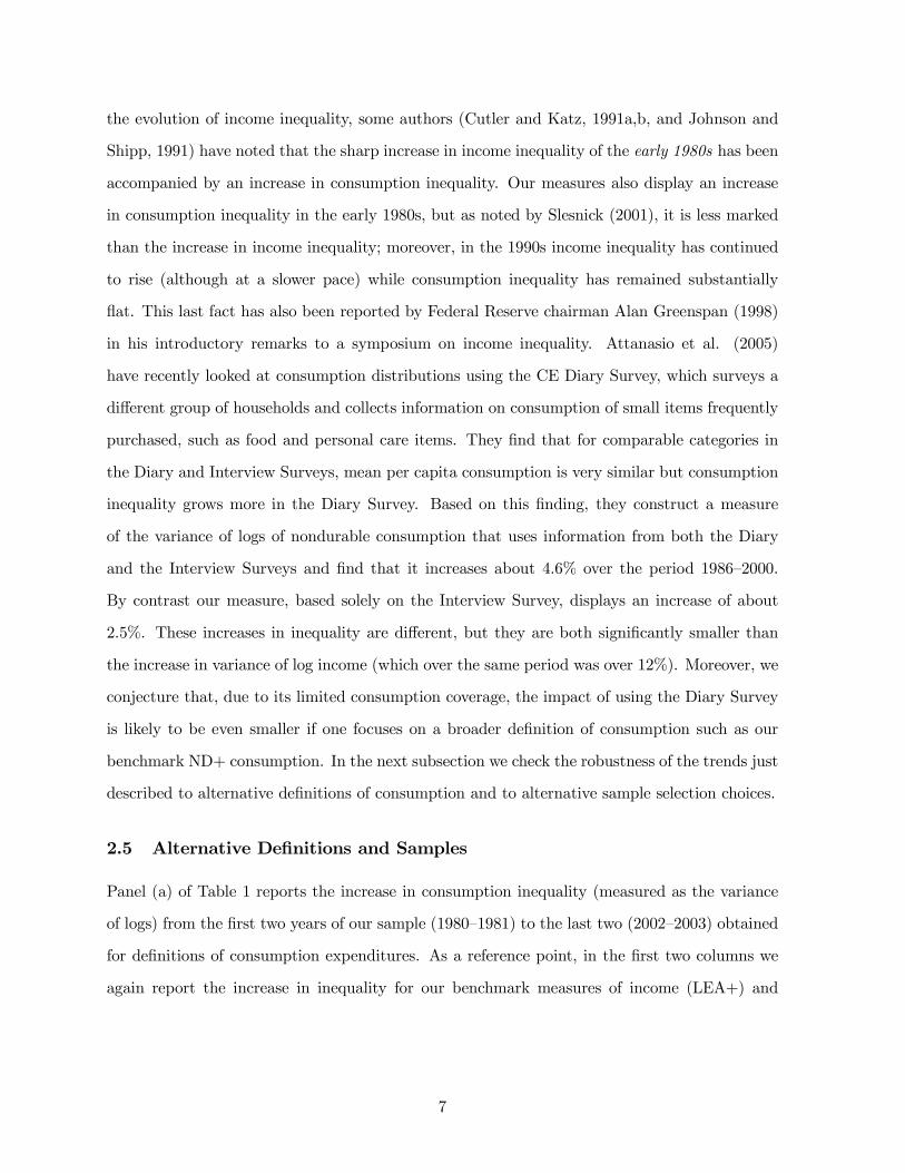
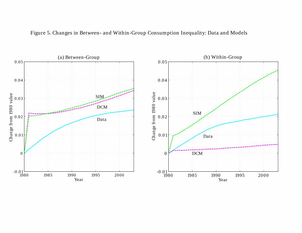
frequency fluctuations. Figure 5 summarizes the main quantitative results of our paper. The

left panel displays the change in the between-group variance of log-consumption implied by both

models as well as the data. The right panel does the same for the within-group variance of

log-consumption, our main focus of interest. Since the sum of the between- and within-group

variance of consumption equals the overall variance, the change in the overall variance from the

data and both models can be readily deduced from the two panels.

Since the change in between-group income inequality is modeled by a deterministic process,

by construction there is no (self-)insurance possible against the increase in between-group income

variability. Thus, in the long run all of the increase in between-group income inequality is

20Since the other statistics are determined exclusively from the production side of the economy, changes in B̄or rb do not require recalibration of A,α, δ.

27

reflected in a one-for-one increase in between-group consumption inequality in both models. It

is therefore not surprising that both models have nearly identical predictions for that part of

consumption inequality. As shown in panel (a) of Figure 2, the fact that in the data the increase

in between-group income inequality is similar to the increase in between-group consumption

inequality implies that the increase in between-group inequality predicted by both models is

similar to the one observed in the data.

The crucial differences between the two models are the financial instruments that can be used

to (self-)insure idiosyncratic income risk, the borrowing limits that constrain the use of these

instruments, and the change of these limits over time. Thus, the crucial quantitative question is

how well both models can capture the trend in within-group consumption inequality. The right

panel of Figure 5 answers this question. It shows that, for our benchmark parameterization, the

DCMmodel understates and the SIM model overstates the increase in within-group consumption

inequality, compared to the data. Although the data display an increase in the variance of about

2.0%, the DCM model shows an increase of only 0.5%, whereas the standard incomplete markets

model predicts an increase of 4.5% compared to the data.21 To put these numbers in perspective,

note that the increase in within-group income variance from the data and fed into the models is

11%. Thus, both models are successful in generating an increase in within-group consumption

inequality that is substantially lower than that for income inequality, in line with the data.

The empirical evidence of increasing both between-group and within-group consumption

inequality also speaks against the standard complete markets model. That model, by allow-

ing perfect consumption insurance between and within groups, counterfactually predicts that

between-group, within-group, and total consumption inequality should remain completely un-

changed over time.

The quantitative difference in the change of within-group consumption inequality in the two

models is due to the differential response of consumer credit to increased income volatility. In

the SIM model the increase in the variance of income leads to higher precautionary savings.

In addition, households facing larger shocks become more hesitant to borrow, plus their ability

21Note that if both panels of Figure 5 are combined, the overall increase in consumption inequality in the datais, even in a quantitative sense, almost perfectly matched by the DCM model. But since this is due to the factthat this model overstates the increase in between-group consumption inequality and understates the increase inwithin-group consumption inequality, we do not want to stress this finding. The SIM model, however, overstatesboth components of inequality and thus the extent of the overall increase in consumption inequality.

28

to borrow remains unchanged. Thus, outstanding unsecured consumer credit (as a fraction

of output) declines by 0.6%, equilibrium asset holdings and thus the physical capital stock

increase by 2.1%, and the real return on capital declines by 17 basis points. In contrast, in

the DCM model credit limits expand for the purchase of all Arrow securities, and households

can and do borrow more, at least against the contingency of having higher income tomorrow.

This is reflected in an increase in outstanding unsecured consumer credit (again, as a fraction

of output) by 2.1%. But keeping consumption as smooth as it was before the change in the

income process may require a bigger expansion in borrowing than is feasible with the new,

wider constraints, so some of the increase in income volatility is reflected in consumption: the

within-group consumption variance increases, albeit only very mildly. The expansion of credit

in the DCM model is met by an increase in purchases of Arrow securities, as households have

a stronger need to save for the contingency of being income-poor tomorrow. On net, aggregate

savings and thus the capital stock increases by 1.8% and the return on capital falls by 15 basis

points. The increase in the capital stock and the decline in the interest rate are smaller than

those in the SIM model because the increase in asset accumulation in the debt constraint model

is partially offset by a higher demand for credit, an effect that is absent in the SIM model. A

precise quantitative evaluation of both models with respect to the CE data along the credit

dimension is not possible because data on unsecured consumer credit are not available in our

CE sample. At least qualitatively, however, the DCM model seems more consistent with recent

developments in U.S. credit markets (see also our Figure 7 in the conclusion).

6.2 Sensitivity Analysis

In this section we document how sensitive our main findings are to changes in the tightness of

the borrowing constraints and the high persistence of the income shock. Finally we assess the

performance of a hybrid model that inherits elements of both the SIM and DCM models.

6.2.1 Borrowing Constraints

In Table 2 we report results for different values of the borrowing constraint for the SIM model.

We normalized the production function in such a way that, in the initial steady state, average

wages are equal to 1. Thus, a borrowing constraint of B = 2 implies that a household can take

29

out (noncollateralized) loans up to twice her annual average labor income. We also document

how our results for the DCM model change if we reduce the net real interest rate at which

households can save in autarky to zero, making the default option less attractive. The statistics

we report are the change, between 1980 and 2003, in the within-group consumption (in logs)

variance, the change in the outstanding credit-to-GDP ratio, and the change in the real interest

rate.

Table 2. Change in Borrowing Constraints

Economy ∆V ar ∆Credit (%) ∆r (%)

SIM, B = 0 0.0456 0 −0.20SIM, B = 1 0.0454 −0.62 −0.17SIM, B = 2 0.0463 −0.88 −0.15DCM, rd = 4% 0.0049 2.05 −0.15DCM, rd = 0% 0.0012 12.34 −0.03

The most important observation from Table 2 is that more generous credit lines per se, if they

do not change over time, do not help to keep the increase in within-group consumption inequality

low in the SIM model. For this result, the existence of capital as an asset in positive net supply

is crucial. Since the wealth-to-output ratio is calibrated to 2.6 in the model, most households

are far to the right from the borrowing constraint in the wealth distribution. In addition, with

highly persistent income shocks, they are very reluctant to obtain credit in response to bad

income shocks. In fact, as these shocks become bigger over time, households become even more

timid in using credit and try to stay away from high debt positions. We observe from the table

that the credit-to-GDP ratio declines with the increase in income volatility, the more so the

looser the borrowing constraint and thus the higher the debt position of those at the constraint.

For the DCM model, reducing the interest rate at which people can save after default leads

to a worse autarkic option, and thus to more borrowing being enforceable. In fact, with an

rd = −2% (i.e., households can save only at a negative real interest rate of 2%), the default

option is so unattractive that perfect risk sharing is possible and the predictions of the DCM

model collapse to those of the standard complete markets model. Reducing the autarkic savings

interest rate gives rise not only to better risk allocation in the initial steady state, but also

to a stronger relaxation of borrowing constraints over time. As a result, the use of credit

30

expands substantially and there is almost no increase in within-group consumption inequality

over time, reducing the ability of the DCM model to match the data relative to the benchmark

parameterization. Also note that with rd = 0%, the increase in credit demand almost matches

the increased savings demand, so that the real interest rate and the capital stock remain virtually

unchanged as income variability increases.

6.2.2 Persistence of Income Shocks

At least since Friedman (1957) it has been well understood that very persistent income shocks are

harder to self-insure against than income shocks that are transitory in nature. Our idiosyncratic

income process is the sum of a highly persistent and a purely transitory component. Although

authors that estimate this process from wage data consistently find the persistence parameter ρ

close to 1, some disagreement exists about its exact magnitude. We have repeated our analysis

for various other choices of ρ and report, in Table 3, results for ρ = 0.8, the value estimated by

Guvenen (2005), which is the lowest estimate for ρ we are aware of, for the exact income process

we use.22 In each case we recalibrate the income process and time discount factor such that the

cross-sectional income dispersion of the process fed into the model matches the empirical facts

from Figure 4, and the initial real return on capital remains at 4%. This procedure keeps the

volatility of the income process unchanged, but reduces its persistence.

Table 3. Change in Persistence: ρ = 0.8

Economy ∆V ar ∆Credit (%) ∆r (%)

SIM, B = 0 0.0355 0 −0.28SIM, B = 1 0.0334 −0.01 −0.22SIM, B = 2 0.0341 0.0 −0.19DCM, rd = 4% 0.0025 1.33 −0.10DCM, rd = 2.5% 0.0013 3.93 −0.04

Comparing the results of Table 3 with those in Table 2, we see that a lower persistence of

income shocks in the SIM model indeed reduces the rise in within-group consumption inequality.22The ρ = 0.8 is the lowest estimate reported in his Table 1. Heaton and Lucas (1996) estimate a simple AR(1)

process; that is, they do not have an independent purely transitory shock. Thus, if the true process is the one weuse, their estimated ρ = 0.53 is a downward-biased estimate of the true autoregressive coefficient.We also repeated our exercises with ρ = 0.95, the value reported by Storesletten et al. (1998). The results,

available upon request, are quite similar to those for ρ = 0.9989.

31

Whereas for ρ = 0.9989 this increase rise was about 4.5%, with ρ = 0.8 it drops to about 3.4%

(compared to 2% in the data). Again, the results are fairly independent of the borrowing

constraint. With lower persistence, households in the SIM model find it easier to self-insure by

accumulating capital and using it to smooth income shocks. The increase in the capital stock

(and corresponding decline in the real return) is more pronounced for ρ = 0.8 than for ρ = 0.9989.

Also, households now are not as timid as before to use credit to smooth income shocks; instead of

a decline of credit as a fraction of GDP, we now observe this statistic to be virtually unchanged.

We conclude that setting persistence of the income shocks to the lower bound from the empirical

literature leads to a lesser increase of within-group consumption inequality in the SIM model.

Still, that model somewhat overstates the increase observed in the data.

In the DCM model, a lower ρ reduces the value of autarky for households with currently

high income whose constraints are binding because it is now less likely that they will remain

income-rich. Thus, ceteris paribus, the implications of the DCM model are closer to those of

the complete markets model. In fact, for ρ = 0.8 any autarkic interest rate below 2% leads

to complete consumption insurance. Thus, although the results for this persistence are not

identical to the complete markets model, they are quantitatively close, making the model’s

understatement of the increase in within-group consumption inequality more severe.

6.2.3 Market Completeness or Endogenous Borrowing Constraints?

There are two main differences between our DCM model and the SIM model.23 First, our model

features a full set of Arrow securities, and second, borrowing constraints adjust endogenously

to changes in the income process. To evaluate whether introducing time-varying borrowing

constraints in the SIM model helps to bring that model’s predictions closer to the data, we now

present results for a hybrid model. This model, named after Zhang (1997), retains the market

structure of the SIM model in that agents can trade only a risk-free, uncontingent bond. The

borrowing constraint, however, is now allowed to vary over time: agents can borrow up to the

maximum amount such that in all possible states tomorrow, they are at least weakly better off

repaying their debt rather than defaulting and living in autarky from there on.

Table 4 displays a crucial lesson: introducing time-dependent borrowing constraints into the

23We thank Pierre-Olivier Gourinchas for helpful discussions leading to this subsection.

32

SIM model, at least in the way proposed by Zhang, does not alter the quantitative implications of

the model with respect to the change in within-group consumption inequality. It does, however,

enable the model to reproduce the empirically observed increase in the use of credit.

Table 4. A Hybrid Model

Economy ∆V ar ∆V ar0 ∆Credit (%) ∆r (%)

SIM, ρ = 0.9989, B = 1 0.0454 0.0095 −0.62 −0.17Zhang, ρ = 0.9989 0.0469 −0.0112 1.7 −0.16DCM, ρ = 0.9989, rd = 4% 0.0049 0.0015 2.05 −0.15SIM, ρ = 0.8, B = 1 0.0334 0.0049 −0.01 −0.22Zhang, ρ = 0.8 0.0348 −0.0154 1.6 −0.22DCM, ρ = 0.8, rd = 4% 0.0025 0.0007 1.33 −0.10

To explain the driving forces behind these results, Table 4 reports not only the change in

within-consumption inequality between the first and last periods of the income transition (the

column labeled ∆V ar), but also the change between the initial steady state and the first period

of the transition (the column labeled ∆V ar0). Households, on impact, respond very differently

to the unexpected change in the income process in the Zhang economy, compared to the SIM

economy. In the Zhang economy, credit lines expand on impact and households make use of

these expanded credit lines. As a result, consumption inequality initially falls. But this comes

at a price: households that have borrowed more now face higher debt levels and income processes

with more extreme realizations. Over time, the debt needs to be serviced, consumption has to

respond, and consumption inequality eventually goes up (about five periods after impact). After

25 years the change in consumption inequality is the same as in the benchmark SIM model.24

Thus, borrowing constraints that are relaxed over time help households in the short run to better

smooth more volatile income fluctuations, but in the long run their debt burden catches up with

them. As a result, consumption inequality does not increase in the short run, but eventually it

does increase to the same extent as in the standard model.

Why doesn’t the same logic apply in the DCM model? Here is where the second feature of

24Another way to explain this is to note that with highly persistent shocks, an increase in the variance ofthese shocks leads to an increase in the cross-sectional variance of permanent income of comparable magnitude,something that Bowlus and Robin (2004) argue occurred empirically in the United States. Not surprisingly, ahigher dispersion of permanent income eventually leads to a larger dispersion of consumption in the SIM model.

33

that model, state-contingent borrowing, comes in. In the DCM model households with currently

high income enter the period with high debt, exactly because they have borrowed against the

contingency of being income-rich. Thus, the high debt is not such a high burden, and households

can and do make use of the higher credit lines without the consequence of particularly low

consumption in the future. In sharp contrast, in the SIM model income-poor people start the

period with outstanding credit (because of the strong positive correlation of income and the

fact that they went into debt because of bad income realizations). Thus, in that model highly

indebted households eventually have to accept (persistently) low consumption. Put another

way, in the SIM model assets and income are highly positively correlated, whereas in the DCM

model they are negatively correlated. Therefore, in one model being in debt has fairly persistent

negative consequences for consumption; in the other model it does not.

7 Conclusions

In this paper we use CE survey data to document that the increase in income inequality for

the United States in the last 25 years has not been accompanied by a substantial increase

in consumption inequality. We propose a theory that provides a simple explanation for this

observation. If the increase in income inequality has been driven, at least partially, by an

increase in idiosyncratic labor income risk, then the value households place on access to formal

and informal credit and insurance mechanisms rises, and the scope of these mechanisms may

endogenously broaden. Individual consumption may then be better insulated against (higher)

income risk, and cross-sectional consumption inequality may increase only mildly. If, however,

the structure of private financial markets and informal insurance arrangements does not respond

to changes in the underlying stochastic income process of individuals, then no further hedging

against the increasing risk is possible, and the increase in income inequality leads to a more

pronounced rise in consumption inequality.

The mechanism through which agents in the DCM model of the last section keep their

consumption profiles stable in the light of more volatile income is an expansion in the use of

noncollateralized credit. Did this expansion take place in the data? One simple (but of course

only partial) measure of credit available that is used by U.S. consumers is the ratio of aggregate

34

unsecured consumer credit to disposable income. In Figure 6 we plot this ratio from U.S. data

for the last 40 years, as well as the Gini coefficient for U.S. household income.25 Despite some

idiosyncratic cyclical variations, the two series display a remarkably similar trend. Combining

this figure with our consumption inequality observations may suggest that consumers could and

in fact did make stronger use of credit markets exactly when they needed to (starting in the

mid-1970s), in order to insulate consumption from bigger income fluctuations. We want to stress

that we view the expansion of credit lines in the DCM model as a metaphor for the expansion of

a variety of formal and informal risk-sharing mechanisms, with formal credit being an important,

but by no means the only, component.

Both models evaluated in this paper have their shortcomings. The DCM model hypothesizes

very well-developed–maybe too developed–direct insurance markets. Although the complete

set of Arrow securities can be interpreted to stand in for the host of assets traded in financial

markets and for informal insurance mechanisms working on the level of the extended family, some

may question the empirical realism of this assumption, which is important for our results, as

demonstrated in the last section. This model is consistent with the empirically observed increase

in credit and the only slight increase in consumption inequality over time. On the one hand,

it overstates the degree to which individual consumption is insulated from income shocks and

understates the response of within-group consumption inequality to increased income volatility.

On the other hand, the SIM model may have a more realistic market structure, but seems to

allow somewhat too little explicit insurance against income shocks, over and above simple self-

insurance. In our application it therefore overstates the level and the increase in within-group

consumption inequality. It also does not display an increase in the use of uncollateralized credit

over time, unless more flexible borrowing constraints are introduced. In their work, Blundell et

al. (2004) and Storesletten et al. (2004) come to the same qualitative conclusion.

Conditional on these findings, we conjecture that a model that, like the DCM, has an endoge-

nous evolution of credit markets but that, unlike the DCM, restricts the insurance possibilities

available to agents (possibly restricting the spanning of the insurance contracts) might be even

25The series for consumer credit is from the 2005 Economic Report of the President, Table B-77. It onlyincludes revolving consumer credit, which is entirely unsecured. The series is available starting from 1968. Personaldisposable income is obtained from the same source, Table B-30. The Gini index for household income is available,starting from 1967, from the U.S. Census Bureau, Historical Income Tables, Table H-4.

35

more empirically successful in matching the data. Further empirical work using micro data may

inform us how to more precisely model the mechanisms that households can use to smooth out

idiosyncratic income shocks. We defer this work to ongoing and future research.

36

ReferencesAiyagari, S. R. (1994), “Uninsured Idiosyncratic Risk and Aggregate Saving,” Quarterly

Journal of Economics, 109, 659—684.

Albarran, P. and O. Attanasio (2003), “Limited Commitment and Crowding Out of Private

Transfers: Evidence from a Randomised Experiment,” Economic Journal, 113, C77—C85.

Alvarez, F. and U. Jermann (2000), “Efficiency, Equilibrium, and Asset Pricing with Risk

of Default,” Econometrica, 68, 775—798.

Attanasio O., E. Battistin, and H. Ichimura (2005), “What Really Happened to Consumption

Inequality in the US?” in E. Berndt and C. Hulten (eds.), Measurement Issues in Economics–

The Paths Ahead: Essays in Honor of Zvi Griliches, University of Chicago Press, Chicago,

forthcoming.

Attanasio, O. and S. Davis (1996), “Relative Wage Movements and the Distribution of

Consumption,” Journal of Political Economy, 104, 1227—1262.

Battistin, E. (2003),“Errors in Survey Reports of Consumption Expenditures,” IFS Working

Papers, W03/07.

Blundell, R., L. Pistaferri, and I. Preston (2004), “Consumption Inequality and Partial

Insurance,” ISF Working Papers, W04/28.

Blundell, R. and I. Preston (1998), “Consumption Inequality and Income Uncertainty,”Quar-

terly Journal of Economics, 113, 603—640.

Bowlus, A. and J.-M. Robin (2004), “Twenty Years of Rising Inequality in U.S. Lifetime

Labour Income Values,” Review of Economic Studies, 71, 709—742.

Cutler, D. and J. Gruber (1996), “Does Public Insurance Crowd Out Private Insurance?”

Quarterly Journal of Economics, 111, 391—430.

Cutler, D. and L. Katz (1991a), “Macroeconomic Performance and the Disadvantaged,”

Brookings Papers on Economic Activity, 1—74.

(1991b), “Rising Inequality? Changes in the Distribution of Income and Con-

sumption in the 1980s,” American Economic Review, 82, 546—551.

Dalaker, J. and M. Naifeh (1998), Poverty in the United States: 1997, U.S. Bureau of the

Census, Current Population Reports Series P60-201, U.S. Government Printing Office, Wash-

ington, D.C.

37

Deaton, A. and C. Paxson (1994), “Intertemporal Choice and Inequality,” Journal of Political

Economy, 102, 437—467.

Díaz-Giménez, J., V. Quadrini, and J.-V. Ríos-Rull (1997), “Dimensions of Inequality: Facts

on the U.S. Distributions of Earnings, Income, and Wealth,” Federal Reserve Bank of Minneapo-

lis Quarterly Review, 21, 3—21.

Dynarski, S. and J. Gruber (1997), “Can Families Smooth Variable Earnings?” Brookings

Papers on Economic Activity, 229—303.

Economic Report of the President, 2005 (2005), Executive Office of the President, Council

of Economic Advisers, Washington, D.C., Table B-77.

Fernández-Villaverde, J. and D. Krueger (2002), “Consumption and Saving over the Life

Cycle: How Important Are Consumer Durables?” mimeo, University of Pennsylvania.

Friedman, M. (1957), A Theory of the Consumption Function, Princeton University Press,

Princeton, N.J.

Gottschalk, P. and R. Moffitt (1994), “The Growth of Earnings Instability in the U.S. Labor

Market,” Brookings Papers on Economic Activity, 217—272.

Gottschalk, P. and T. Smeeding (1997), “Cross-National Comparisons of Earnings and In-

come Inequality,” Journal of Economic Literature, 35, 633—687.

Greenspan, A. (1998), “Opening Remarks to the Symposium on Income Inequality: Issues

and Policy Options,” Federal Reserve Bank of Kansas City.

Guvenen, F. (2005), “Learning Your Earning: Are Labor Income Shocks Really Very Persis-

tent?” mimeo, University of Rochester.

Heathcote J., K. Storesletten, and G. Violante (2004), “The Macroeconomic Implications of

Rising Wage Inequality in the US, ” mimeo, Georgetown University.

Heaton, J. and D. Lucas (1996), “Evaluating the Effects of Incomplete Markets on Risk

Sharing and Asset Pricing,” Journal of Political Economy, 104, 443—487.

Huggett, M. (1993), “The Risk-Free Rate in Heterogeneous-Agent Incomplete-Insurance

Economies,” Journal of Economic Dynamics and Control, 17, 953—969.

Johnson, D. and S. Shipp (1991), “Trends in Inequality Using Consumer Expenditures:

1960 to 1993,” Proceedings of the Section on Survey Research Methods, American Statistical

Association, 1—7.

38

Johnson, D. and T. Smeeding (1998), “Measuring the Trends in Inequality of Individuals

and Families: Income and Consumption,” mimeo, Bureau of Labor Statistics.

Katz, L. and D. Autor (1999),“Changes in the Wage Structure and Earnings Inequality,”

in O. Ashenfelter and D. Card (eds.), Handbook of Labor Economics, vol. 3A, North-Holland,

Amsterdam.

Kehoe, T. and D. Levine (1993), “Debt Constrained Asset Markets,” Review of Economic

Studies, 60, 865—888.

(2001), “Liquidity Constrained Markets versus Debt Constrained Markets,”

Econometrica, 69, 575—598.

Kocherlakota, N. (1996), “Implications of Efficient Risk Sharing without Commitment,”

Review of Economic Studies, 63(4), 595—609.

Krueger, D. and F. Perri (1999), “Risk Sharing: Private Insurance Markets or Redistributive

Taxes?” Federal Reserve Bank of Minneapolis Staff Report 262.

(2004),“On the Welfare Consequences of the Increase in Inequality in the United

States,” NBER Macroeconomics Annual 2003, 83—121.

Mayer, S. and C. Jencks (1993), “Recent Trends in Economic Inequality in the United

States: Income versus Expenditures versus Well-Being,” in D. Papadimitriou and E. Wolff

(eds.), Poverty and Prosperity in the USA in the Late Twentieth Century, St. Martin’s Press,

New York.

McGrattan, E. and E. Prescott (2003), “Average Debt and Equity Returns: Puzzling?”

American Economic Review, 93, 392—397.

Nelson, J. (1994), “On Testing for Full Insurance Using Consumer Expenditure Survey Data:

Comment,” Journal of Political Economy, 102, 384—394.

Pendakur, K. (1998), “Changes in Canadian Family Income and Family Consumption In-

equality between 1978 and 1992,” Review of Income and Wealth, 44, 259—283.

Slesnick, D. (1993), “Gaining Ground: Poverty in the Postwar United States,” Journal of

Political Economy, 101, 1—38.

(2001), Consumption and Social Welfare: Living Standards and Their Distrib-

ution in the United States, Cambridge University Press, Cambridge.

Storesletten, K., C. Telmer, and A. Yaron (1998), “The Risk Sharing Implications of Alter-

39

native Social Security Arrangements,” Carnegie-Rochester Conference Series on Public Policy,

50, 213—59.

2004, “Consumption and Risk Sharing over the Life Cycle,” Journal of Monetary

Economics, 51, 609—633.

Tauchen, G. and R. Hussey (1991), “Quadrature-Based Methods for Obtaining Approximate

Solutions to Nonlinear Asset Pricing Models,” Econometrica, 59, 371—396.

U.S. Census Bureau (2004), “Gini Ratios for Households, by Race and Hispanic Origin of

Householder: 1967 to 2000,” http://www.census.gov/hhes/income/histinc/h04.html.

Violante, G. (2002), “Technological Acceleration, Skill Transferability and the Rise in Resid-

ual Inequality,” Quarterly Journal of Economics, 117, 297—338.

Zhang, H. (1997),“Endogenous Borrowing Constraints with Incomplete Markets,” Journal

of Finance, 52, 2187—2209.

40

Appendix A Data DescriptionIn this appendix we provide a detailed description of the income and consumption data we use

in the paper.

A.1 CE Files and ObservationsOur data come from the CE Interview Surveys 1980 through 2003 (which also contain data

for the first quarter of 2004) provided by the Bureau of Labor Statistics (BLS). Consumption

expenditure data are from the Family Characteristics and Income (FAMILY) files except for the

years 1982 and 1983, for which the FAMILY files do not contain consumption information. For

those years we obtain consumption data from the Detailed Expenditures (MTAB) files. Note that

the consumption information in the FAMILY files is just an aggregation of the information in the

MTAB files. Income data are from the FAMILY files and hours worked by household members

(used to construct wages) are from the Member Characteristics and Income (MEMBER) files.

An observation in our data set consists of all the information collected in a given interview for

a given household (identified by a unique ID number). Each household is present in no more

than four observations.

A.2 Consumption CategoriesIn Table A1 we report all the categories of consumption expenditures we use, together with the

BLS price index we use to deflate them. Categories 1 through 20 are reported directly in the CE

for every observation, and we derived categories 21 and 22 as described below. Our definition

of ND consumption (used in Table 1) includes categories 1 through 13. Our measure of ND+

consumption includes ND consumption, categories 20 and 21, plus categories 14 though 18.

These latter categories contain expenditures on durable goods, but since we do not have enough

information to compute imputed services from those durables, we simply include expenditures.

Finally, our definition of total consumption expenditures (used in Table 1) includes categories 1

through 20. We now describe in more detail some of the categories.

A.2.1 Food Expenditures CorrectionA change in survey methodology (see Battistin, 2003, for details) causes a sizeable (about 15%)

systematic downward bias in reported food expenditures for all the observations in the years

1982—1987. In order to correct for this bias, we regress the log of food expenditures for all years on

a quadratic time trend, on quadratics in income and total nonfood consumption expenditures,

on weeks worked, on a complete set of household characteristics (including age, education,

region of residence, and family composition), on a dummy for the period 1982—1987, and on the

interactions term of the dummy with all other independent variables. We then use the regression

coefficients to scale up food expenditures for every observation in the period 1982—1987.

A.2.2 Services from VehiclesEach CE observation contains reports of expenditures for purchases of new and used vehicles.

The CE also reports the number of cars owned by the household in that quarter. For each year

we first select all observations that report positive expenditures for vehicle purchases, and run

41

a regression of these expenditures on quadratics in income and total nonvehicle consumption

expenditures, weeks worked by household members, expenditures on gasoline, expenditures on

public transportation, vehicle maintenance expenditures, the number of cars owned, a complete

set of household characteristics (including age, education, region of residence, and family com-

position), plus quarter dummies. These regressions have an R2 that ranges from 74% to 94% in

our sample years. On average, in every year a little more than 10% of households report positive

expenditures on vehicles. We use the estimated regression coefficients to predict expenditures for

vehicles for all households in that year (i.e., for those who did and for those who did not report

positive vehicle expenditures). Our measure of consumption services from vehicles, then, is the

predicted expenditures on vehicles, times the number of cars the consumer unit owns, times 132

(reflecting the assumption of average complete depreciation of a vehicle after 32 quarters).

A.2.3 Services from Primary ResidenceEach observation in the CE provides information on whether the household rents or owns its

primary residence. If the household rents, we measure housing services as the rent paid, including

insurance and other out-of-pocket expenses paid by the renter. To impute housing services for

those households that own, we use a variable from the CE that measures the market rent (as

estimated by the reference person of the consumer unit) the residence would command if rented

out. This variable is not available for all years of the sample, in particular not for the years

1980—1981 and 1993—1994. Thus, in order to compute this variable in a uniform way across our

sample, we use an imputation procedure similar to the one used for vehicles. For the year for

which we have the reported market rent of the unit, we regressed it on self-reported property

values, quadratics in income and total nonhousing consumption expenditures, a complete set of

household characteristics (including age, education, region of residence, and family composition),

plus quarter dummies. Since property values are reported by only a subset of the home owners,

we allow the coefficient of the regression to be different for those who reported the property

value from those who did not. These regressions have an R2 that ranges from 30% to 55%

in our sample years. We then use estimated regression coefficients to predict the rental value

of owned properties for all the home owners. For the years 1980—1981 we use the coefficient

estimated in 1982, and for the years 1993—1994 we use the coefficients estimated in 1995. For

the years 1982—1992 and 1995—2003, we have both the actual and the imputed rental equivalent

of the owned home, so we computed the trends in consumption inequality using housing services

computed in both ways. The resulting trends are extremely similar.

A.3 Sample SelectionWe first exclude observations for which there is clear evidence of measurement error. In par-

ticular we exclude observations classified as incomplete income respondents, observations that

report zero food expenditures for the quarter, those who report only food expenditures for the

quarter, and those who report positive labor income but no hours worked. We then exclude all

observations with an age of the household head below 21 or above 64, and those with negative

or zero LEA+ earnings. In our benchmark sample we also exclude observations with weekly

42

wages of the reference person below half of the minimum wage, households classified as rural,

and those households that have not completed the full set of four interviews.

A.4 Aggregation and Top-CodingInequality measures are computed on annual cross sections. We assign an observation to a given

year if the last interview of that household is completed between April of that year and March of

the following year. Whenever income or consumption expenditures are top-coded, we set them

to their top-coding thresholds. We have experimented with increasing the values of top-coded

income/consumption components (multiplying the threshold by 1.5). Inequality measures are

robust to these changes because in general, the number of observations with top-coded income

or consumption figures never exceeds 2% in a given quarter.

A.5 Data AvailabilityOur data set in Stata format, including brief documentation, is available at http://pages.stern.

nyu.edu/~fperri/research_data.htm.

Appendix B Recursive Formulation and Computational AlgorithmIn this appendix we formulate the consumer problem for the DCM model recursively and provide

a sketch of the algorithm used to compute a stationary equilibrium. In the nonstationary case

(that is, along the transition), the logic remains the same but all functions have to be indexed

by t. For simplicity here we omit the distinction by types and lump into y the transitory and

persistent income shocks. The equilibrium problem is nonstandard because one needs to solve

not only for prices but also for endogenous borrowing constraints. We first compute the value

of autarky as the fixed point to the functional equation

UAut(y, b) = maxc,b0≥0

⎛⎝(1− β)u(b+ y − b0

1 + rd) + β

Xy0∈Y

π(y0|y)UAut(y0, b0)

⎞⎠ .

We then guess the risk-free rate R = 1/q. No arbitrage implies that the prices of the Arrow

securities q(y0|y) are a function of our guess and are given by qπ(y0|y). We guess borrowingconstraints Ai(y0) and solve the consumer problem, taking these borrowing constraints Ai(y0)and prices for Arrow securities qπ(y0|y) as given:

V (y, a) = maxc,{a0(y0)}y0∈Y

⎧⎨⎩(1− β)u(c) + βXy0∈Y

π(y0|y)V (i, a0(y0), y0)⎫⎬⎭

s.t.

c+Xy0∈Y

q(y0|y)a0(y0) = αiy + a a0 ≥ Ai(y0).

We finally check to make sure the borrowing constraints are not too tight by asking whether

V (y0, Ai(y0)) = UAut(y0, 0)

43

for all y0. If the equalities hold, then we have solved for the borrowing constraints associated withthe guessed interest rate; if not, we update the guesses for Ai(y0) until all equalities hold. Oncewe have found the borrowing constraints that are not too tight, we use the associated optimal

asset policies a0(y, a; y0) together with the transition probabilities π to define the operator Hthat maps current measures over wealth and income shocks into tomorrow’s measures. We then

compute the (unique) fixed point of the operator H and denote it by Φ. Given Φ and the optimal

consumption policies, we can check the market clearing conditions. If market clearing holds, we

have found a stationary equilibrium; if not, we update our guess of the interest rate R = 1q .

We implement this procedure numerically by approximating value and policy functions with

piecewise linear functions over the state space. For more details on the basic algorithm and on

the theoretical characterization of the stationary equilibrium, see Krueger and Perri (1999).

44

Table A1. Consumption Categories and Deflators

Number Category CPI Used to Deflatea

Nondurable Expenditures

1 Food Food SAF12 Alcoholic beverages Alcoholic beverages SAF1163 Tobacco Tobacco and smoking products SEGA4 Personal care Personal care SAG15 Fuels, utilities, and public services Fuels and utilities SAH26 Household operations Household furnishings and operations SAH37 Public transportation Public transportation SETG8 Gasoline and motor oil Motor fuels SETB9 Apparel Apparel SAA

10 Education Tuition expenditures SEEB11 Reading Recreational reading material SERG12 Health services Medical care SAM

13 Miscellaneous expendituresb Miscellaneous personal services SEGD

Other Expenditures

14 Entertainment Entertainmentc SA615 Household equipment Household furnishings and operations SAH3

16 Other lodging expensesd Shelter SAH1

17 Other vehicle expensese Car maintenance and repair SETD18 Rented dwellings Rent of primary residence SEHA19 Owned dwellings Shelter SAH120 Purchases of vehicles Purchase of new vehicles SETA01

Imputed Services

21 Services from owned primary residence Rent of primary residence SEHA22 Services from vehicles Purchase of new vehicles SETA01

a CPI are monthly average city data for all urban consumers, not seasonally adjusted, and are in base 1982–1984 = 100.b Mostly fees for services such as banking or legal assistance.c BLS CPI for entertainment ends in 1998. We extend it to 2004 using the CPI for recreation (SAR).d Includes mostly expenditures on vacation homes.e Includes expenditures on maintenance, repairs, insurance, and finance charges.

BLS CPI Code

Table A2. Summary Statistics for the Benchmark Sample

Year Households Average IncomeLEA+ ND ND+

1980 638 15736 7447 129401981 1439 15419 7348 128751982 1313 16453 6949 126051983 1700 16746 7134 128731984 1771 18017 7398 134951985 1267 17862 7323 134631986 748 18678 7308 137251987 1840 19318 7558 139921988 1621 18881 7391 137521989 1762 19585 7517 141831990 1789 18893 7455 141711991 1749 19170 7376 138581992 1725 19046 7126 137371993 1786 18841 7115 136861994 1744 18657 7114 134981995 1325 19269 7127 138651996 881 20203 7433 146741997 1609 20557 7203 142041998 1578 20952 7323 146891999 1763 22060 7263 145322000 2164 21508 7191 145082001 2227 21468 6967 140602002 2387 23427 7280 147662003 2593 22544 7053 14359

Note: Income and consumption measures are in 1982–1984 constant dollars per adult equivalent.

Averages are weighted using CE population weights. A household belongs to year x if

its fifth interview is between the second quarter of year x and the first quarter of year x +1.

Average Consumption

1980 1985 1990 1995 20000.2

0.25

0.3

0.35

0.4

Figure 1. The Evolution of Income and Consumption Inequality in the United States, 1980-2003

Gini Index

1980 1985 1990 1995 20002

3

4

5

6

7

Year

90/10 Ratio

1980 1985 1990 1995 20001.5

2

2.5

350/10 Ratio

1980 1985 1990 1995 20000.1

0.2

0.3

0.4

0.5

0.6

Variance of Logs

ND+ Consumption LEA+ Income 2SE BandsNote: The standard errors are computed using a bootstrap procedure with 100 repetitions

1980 1985 1990 1995 2000-0.02

0

0.02

0.04

0.06

0.08

0.1

0.12

0.14

0.16

Ch

ange

fro

m 1

98

0 v

alu

e

Year

Figure 2. Changes in Between- and Within-Group Income and Consumption Inequality

(a) Between-Group

Income

Consumption

1980 1985 1990 1995 2000-0.02

0

0.02

0.04

0.06

0.08

0.1

0.12

0.14

0.16

Ch

ange

fro

m 1

98

0 v

alu

e

Year

(b) Within-Group

Income

Consumption

Figure 3. Characterizing the Link Between Income and Consumption Dispersion

Val

ues

U(1+r+ε)

U(1-ε)

U(1+ε)

ε1

ε(r) ε(r)εb

εa

εc(ε

b)

Income dispersion, ε

Inco

me

and

Con

sum

pti

on D

isp

ersi

on

Income Dispersion

Consumption Dispersion

εc(ε

a)

Income dispersion, ε

UFB(r)

ε(r) ε(r)ε1

0

1980 1985 1990 1995 20000.05

0.1

0.15

0.2

0.25

0.3

0.35

0.4

0.45

0.5

0.55Figure 4. Income Variances: Data and Models

Var

ian

ce

Year

σ2y

σ2α

σ2z

σ2ε

Note: The solid lines are the time series of the cross-sectional variances estimated in the data. The dashed lines (which are the solid lines HP filtered) are the cross-sectional variances used in the models.

1980 1985 1990 1995 2000-0.01

0

0.01

0.02

0.03

0.04

0.05

Year

Ch

ange

fro

m 1

98

0 v

alu

e

Figure 5. Changes in Between- and Within-Group Consumption Inequality: Data and Models

(a) Between-Group

SIM

DCM

Data

1980 1985 1990 1995 2000-0.01

0

0.01

0.02

0.03

0.04

0.05

Year

Ch

ange

fro

m 1

98

0 v

alu

e

(b) Within-Group

SIM

Data

DCM

1965 1970 1975 1980 1985 1990 1995 2000 20050.38

0.4

0.42

0.44

0.46

0.48Figure 6. Income Inequality and Consumer Credit

Consumer Credit

Income Inequality

Inco

me

Gin

i

Years1965 1970 1975 1980 1985 1990 1995 2000 2005

0

0.02

0.04

0.06

0.08

0.1

Non

-sec

ure

d C

onsu

mer

Cre

dit

ove

r P

erso

nal

Dis

pos

able

In

com

e