Does the Environmental Kuznets Curve Describe How...

Does the Environmental Kuznets Curve DescribeHow Individual Countries Behave?Robert T. Deacon and Catherine S. Norman

ABSTRACT. We examine within-country timeseries data on income and concentrations of SO2,smoke, and particulates to see if the shapes ofpollution-income relationships in individualcountries agree qtialitatively with predictions of theenvironmental Kuznets curve. The shapes of the.serelationships are determined non-parametricaltyfor individual cotintries using recently availabledata on air pollution concentrations. Eor smokeand particulates, the shapes of within-country,polltition-income patterns do not agree with theEKC hypothesis more often than chance wotitddictate. For SO2. which generally exhibits EKC-consistent pollution-income relationships amongwealthier countries, the observed patterns are alsoconsistent with a simpler hypothesis. (JEL Q20,013)

I. INTRODUCTION

The environmental Kuznets curve (EKC)is an empirical proposition about the rela-tionship between a country's income andits levels of pollution. Starting from an ini-tially low income level, the EKC postulatesthat, as a country's income grows, its pollu-tion will initially rise, but will eventuallydecline if growth proceeds far enough, trac-ing out an inverted-U relationship. Thereis now an extensive empirical literature onthe EKC. We contribute to this literatureby examining time series data on pollutionand income for individual countries andpollutants to see if the EKC's qualitativepredictions are borne out with greater fre-quency than chance would dictate. In con-trast to the majority of EKC studies, wefocus exclusively on within-country em-pirical relationships. We believe evidencefrom within individual eountries can po-tentially provide compelling evidence on

Land Economics • May 2006 • 82 (2); 291-315ISSN 0023-7639; E-ISSN 1543-8325© 2006 by the Board of Regents of theUniversity of Wisconsin System

the central policy question at issue in thisliterature: how will an individual nation'senvironmental quality evolve if it makesthe transition from poverty to affluence?Unlike other studies, we test a very gen-eral form of the EKC hypothesis: that acountry's pollution-income relationship canbe described by a single peaked curve, whichmay be particular to an individual countryrather than common across countries.

The empirical strategy tests three im-plications of the EKC hypothesis: incomegrowth is accompanied by increased pollu-tion in low-income countries, by decreasedpollution in high-income countries, and byfirst increasing, then decreasing, pollu-tion in middle-income eountries. To reducethe number of shapes possible in anypollution-income plot, within-country pol-lution and income data are collapsed bytaking means over three country-specificincome ranges. The three summary datapoints that result are then plotted and theirshapes examined. The "shape" (increasing,decreasing, inverted-U, etc.) of a pollution-income plot for a particular country andpollutant is treated as an observation. Intotal, 52 such observations are examined forconsistency or inconsistency with the EKCpredictions. The tests are for "qualitative

The authors are, respectively, professor of econom-ics, University of California. Santa Barbara and univer-sity fellow. Resources for the Future; and assistantprofessor. Department of Geography and Environmen-tal Engineering, The Johns Hopkins University,

This material is based on work supported by NSFGrant No. 9S08696, Without implicating them tor errors,the aulhors aeknowledge valuable comments from EdBarbier. Henning Bohn, Chris Costello. Bill Harbaugh,John List, Doug Steigerwald, David Stern. DavidMolloy Wilson, and two anonymous referees, ArikLevinson kindly provided an updaled version of theGEMS dataset. An earlier version of this paper wasincluded as part of Catherine Norman's PhD disserta-tion at the University of California, Santa Barbara.

292 Land Economics May 2006

consistency" with the EKC in the followingsense: a particular pollution-ineomc plot isjudged EKC-consistent if some single-peaked curve, whdse peak falls in a rangeof possible EKC turning points identifiedfrom the literature, can be drawn through it.Tlie central conclusion from this analysis isthat, with one notable exeeption, the shapesof observed pollution-ineome relationshipsdo not agree with EKC predictions with anygreater frequency than random data would.

The EKC has now been studied exten-sively. Despite numerous critiques, its cen-tral policy message —that the simultaneouspursuit of economic growth and a cleanerenvironment ultimately need not conflict-remains influential. Part of the EKCs ap-peal, particularly to non-specialists, is thatit seems to agree with environmentalchanges observed in the world's wealthiernations over the last 50 years. Casual em-piricism suggests that environmental qual-ity in many of these countries worsenedfollowing World War II, but eventually im-proved after the late l%Os. Because in-comes generally were increasing over thisperiod it is tempting to conclude that aninverted-U proeess, with income as thedriving force, was at work.' We believe thisplausible eonjeeture deserves more earcfulscrutiny, and set out here to see if it is sup-ported across a series of countries and airpollutants by available, widely used data.

The following section reviews the EKCliterature, Seetions 3 and 4 describe the non-parametric approach and the data used to

IIS, airborne emissions of carhon monoxide andvolatile organic compounds show an invortod-LI shapewhen ploltcd over time, and sulfur dioxide (SOT) dis-plays a single peak if WWII years arc excluded (U. S.Environmental Protection Agency 2(HM)), which roughlyagrees with the generalization in the text. Other pollut-ants show different patterns, however. Over availablereporting periods, IIS. air emissions were monotonieallyincreasing for nitrogen oxide, decreasing for lead andPMIO particulates, and roughly constant for finer par-ticulates. Further, an inverted-U relationship heiweenpollution and time (as with carhon monoxide and vol-atile organic compounds) eomhined with an increas-ing relationship between income and time need notresult in an invcrtcd-LI relationship hetween pollutionand income.

examine within-country, pollution-incomerelationships and Section 5 presents testsfor nonrandomness in the shapes of within-country, pollution-income plots. These testsreveal that EKC-consistent behavior in oursample largely consists of SO^ cleanup thatoccurred in wealthy countries while theywere growing. Following up on this point.,Section 6 carries out a time series analy-sis of within-country data to see if theEKC model ean add explanatory power toa simple alternative specification in whichpollution declined over time in richer coun-tries, possibly due to changes in informa-tion, technology, or preferences.

II. EMPIRICAL AND THEORETICALWORK ON THE EKC

The EKC first emerged in studies of am-bient concentrations of air and water pol-lution data collected by the World HealthOrganization and reported under the nameGlobal Environmental Monitoring Sys-tem (GEMS). Shafik and Bandyopadhyay(1992) estimated cross-country relation-ships between income and air and waterpollution, deforestation and waste output,concluding that airborne SO^ and smokeconcentrations began to diminish after anincome level of $3,{)00-$4,000 per capitawas reached. Grossman and Krueger (1993)reached similar conclusions from an analy-sis of the same data, but found turningpoints in the $4,()()()-$6.()0() range. Gross-man and Krueger (1995) confirmed theinverted-U pattern for some additional en-vironmental measures, but with turningpoints at different ineome levels. Panayotou(1997) controlled for industrial structureto allow for the possibility that productionshifts toward cleaner products as incomegrows, and Torras and Boyce (1998) andBarrett and Graddy (2000) included mea-sures of literacy, economic inequality., andcivil and political freedoms in the analysis.In each case, the inverted-U was confirmedusing the GEMS data set. Harbaugh,Levinson, and Wilson (2002) (hereafterHLW) examined an expanded and cor-rected version of the GEMS data used inearlier research. ITiis later version included

82(2) Deacon and Norman: Kuzrtets Curve and How Countries Behave 293

more observations and corrected some er-roneous entries found in versions used inearlier research. HLW found no clear sup-port for the inverted-U relationship andobtained results that were sensitive to sam-ple, specification, and estimation method.'

While the preceding studies all exam-ined ambient concentrations, a parallelstrand of research focused on nationwidepollution emissions. Hilton and Levinson(̂ 1998) separated the policy response (pol-lution per unit output) from the scale effectfor lead emissions. They identified an EKCwith a turning point in the normal range.but found it was sensitive to specificationand sample period. Seiden and Song (1994)examined airborne emissions of SO2 andparticulates in a panel of mostly OECDnations. They found the EKC pattern, butwith turning points in the $8,000-10,000income range. Holtz-Eakin and Seiden(1995) examined CO2 emissions, an unreg-ulated pollutant at the time, and found nopoint at which emissions declined with totalincome. Stern and Common (2001) exam-ined SO2 emissions and found a "turningpoint" exceeding $100,000, far outside theobserved range of per capita income. Theyalso found different turning points for sep-arate samples of OECD and non-OECDcountries, suggesting that searching for auniversal EKC may be inappropriate."

Relatively few empirical studies haveevaluated the EKC by looking at incomeand pollution within countries, over time.Among these, De Bruyn (1997) examinedtime series data on income and sulfur emis-sions in four OECD nations separately andfound relationships that took a variety ofshapes, including Us and Ns, in addition

"' Antweiler, Copeland, and Taylor (2001) used theGEMS data to examine a model of pollution generationthat separates scale, technique, and output compositioneffects, but without testing the EKC hypothesis directly.

' Cole {2003) estimated :m EKC niodel that allowsemissions to respond to differences in openness :md com-parative advantage and concludes that the inverted-Uis not driven by considerations of trade. Lopez andGalinato (2005) show that the position of an EKC forforest cover is significantly related to trade openness andgovernance.

to the inverted-U. Vincent (1997) tested pre-dictions from the EKC literature on a panelof detailed data from Malaysian states. Hefound that parameters from published EKCmodels failed to predict the pattern ofchanges in Malaysian air and water pollu-tion; moreover, none of the Malaysian pol-lution measures exhibited an EKC at all.Perman and Stern (2(X)3) studied sulfuremissions and, after accounting for the timeseries properties of emissions data, foundno statistical support for the EKC hypoth-esis either in a panel or in within-countryanalysis. Notably, the preceding within-country studies were based on emissionsrather than concentrations and none con-firmed the inverted-U as a valid general-ization. Markandya, Pedroso. and Golub(2(X)4) estimated within-country pollution-income regressions for SO2 emissions in 14European eountries. They found a quadrat-ic, inverted-U relationship fit best in fourcases, but the other significant relationshipswere complex fourth order polynomials.

Other researchers have examined paneldata from US states. Carson, Jeon, andMcCubbin (1997) estimated EKCs for airquahty and found that most measures im-proved monotonically with income overthe sample range. List and Gallet (1999)studied sulfur and nitrogen emissions in apane! of U.S. states over the period 1929-1994. They found evidence that forcingthe same specification (and hence turningpoint) on all the states resulted in biasedestimates. Using the same data, Miliimet,List, and Stengos (2003) found the EKCpeak to be highly sensitive to modelingassumptions and rejected a parametrie spec-ification in favor of a more flexible semi-parametric approach."^ Stem (2004,1424-25)provides a critical overview of EKC papersexamining airborne sulfur and their variouseconometrie approaches.

•* Koop and Tole (1999). in their examination ofdeforestation in a cross-country setting, also foundevidence that the shape of income-forest cover rela-lionsliips varied considerably across countries. Inter-estingly, they found an inverted-U relationship onlywben they imposed ii single functional form on all Ihecountries observed.


The emergenee ofthe inverted-U in em-pirical work prompted a theoretical liter-ature to explain how this shape mightarise.^ Stokey (1998) showed that it couldemerge from a model in which pollutioncontrol effort is not expended until a pol-lution threshold is crossed. Andreoni andLevinson (2001) demonstrated that strongincreasing returns to scale in pollutionabatement could give rise to an inverted-U.Lopez and Mitra (1997) showed how cor-ruption in government, by reducing abate-ment effort, could affect the shape of theEKC and move its turning point.^ Brockand Taylor (2004) showed that an EKC-like relationship could arise naturally in aSolow growth model, but demonstratedthat the peak could occur at virtually anyincome level. Copeland and Taylor (2003,chapter 3) examined four mechanisms thatcan generate an inverted-U in the contextof a single consistent modeling framework,effectively summarizing much of this work.^

The EKC has now been extensively re-searched and the associated literature hasbeen reviewed and critiqued. Despite thisconcerted attention, the literature remainsincomplete in two respects. First, examplesof countries actually moving up one side ofthe inverted-U curve and down the otherhave yet to be identified in the literature.Indeed, time series analysis of individualcountries has yielded disappointing results;see De Bruyn (1997), Vincent (1997), andPerman and Stern (2003). Second, severalresearchers have concluded that the shapesof pollution-income relationships may becountry specific, so generic empirical speci-fications may yield biased results. This pointis made by Stern, Common, and Barbier

Given the empirical emphasis in this paper, the-oretical contributions are summarized only briefly. Stern(2()()4, 1420-22) reviews mueh of this work and providesan extensive hibliography,

" Weisch (2004) tests one implication of ihis theoryand finds a sirong, positive relationship hetween pol-lution and corruption when income is held eonstanl,

•' Israel and Levinson (2(X)4) use data from theWorld Values Survey to test ancillary predictions fromdifferent theoretical models that have heen used lo gen-erate the EKC.

(1996), by Barbier (2001) in his review ofempirical work on tropical forest cover, andin Coondoo and Dinda's (2002) discussionof causality in EKC studies. It is corrobo-rated by results from Hilton and Levinson(1998).' HLW. and Stern and Common(2001) indicating the sensitivity of EKCresults to sample. In addition, theoreticaltreatments by Lopez and Mitra (2000) andBrock and Taylor (2004) indicate that a singleEKC function need not fit all economies.

in. EMPIRICAL APPROACH

The empirical approach followed here ismotivated by these observations on the lit-erature. First, attention is focused exclu-sively on pollution-income patterns withinindividual countries, over time. The appealof the EKC is its potential ability to predicthow a eountry's pollution will change as itseconomy grows. To policymakers, the iden-tification of countries behaving accordingto the EKC proposition for specific pol-lutants would be compelling evidence forthe theory's value. In addition, examiningonly within-country data minimizes the in-fluence of cross-country heterogeneity, re-stricting this source of potential concernto attributes that change within a countryduring the sample period. While recogniz-ing the power of panel data methods,which have been the foundation of pastEKC research, empirical applications in theEKC literature have required sueh hetero-geneity to be additive and this may be toorestrictive. Allowing individual countries tofollow different pollution-ineome pathsmay yield new insights.

Second, to impose minimal structure onthe shapes of pollution-income relation-ships in individual countries, a nonpara-metric method is used to characterize theshapes of these relationships qualitatively,that is. as monotone increasing, monotonedecreasing, single peaked, etc. A country'spollution-income relationship is then char-acterized as EKC-consistent if it followssome single peaked function whose peakfalls within a speeified range. The rangeused in practice, while motivated by EKCpeaks reported in the literature, is very

82(2) Deacon and Norman: Kuznets Curve and How Countries Behave 295

broad. According to the EKC hypothesis,ineome growth should be associated withincreasing pollution in poor countries andwith decreasing pollution in rich countries,where poor and rich refer to whether acountry's observed ineome series lies en-tirely to the left or to the right of the rangeof possible EKC peaks. When a country'sincome series lies partially or entirely with-in the range of allowed peaks, a variety ofpollution-income shapes are potentiallyEKC-consistent, as explained shortly. Test-ing the predictive power of the EKC hy-pothesis involves determining whether ornot EKC-consistent shapes occur more fre-quently in the observed data than would bethe case in randomly generated data.

The shapes of pollution-income relation-ships are identified non-parametrically bycollapsing the available annual observationson pollution and income for each pollutant-country case examined into three summaryobservations. First, the country's pollutionand ineome observations are ordered byincome, measured as real GDP per capita.These observations are then partitioned intotritiles. three groups that eontain the lowest,middle, and highest third of that eountry'sGDP observations. Next, mean GDP andmean pollution for each tritile are computed,yielding three summary poilution-ineomepoints for the country-pollutant case underconsideration. The plot of these points is thenexamined to see if they ean be connected bysome single-peaked curve whose peak liesin a specified range of possible EKC turn-ing points. Thus, monotone-inereasing andmonotone-decreasing, pollution-incomeplots can satisfy this criterion for incomeranges that lie. respectively, entirely below orentirely above the range of possible EKCpeaks. If a country's range of GDP observa-tions lies partially or entirely within therange of possible turning points, more thanone shape can satisfy the criterion. Detailedcriteria and the range of EKC turning pointsapplied in these tests are provided follow-ing the presentation of summary statistics.

This procedure is illustrated in Figure 1using data for four of the countr>'-pollutantcases examined. Panels A and B show 21annual observations (from 1972-1992) for

GDP and sulfur dioxide in two countries,Canada and Japan.'̂ The vertical lines showthe GDP cutoff levels that partition eachcountry's observations into tritiles. The circlesshow mean pollution and GDP in each tritile.Thc plot of these three points in Panel A,depicting Canada, decreases monotonically.This shape is EKC-consistent because Cana-da's GDPobservations lie above the range ofestimated SO2 turning points reported in theliterature. The plot for SO2 in Japan, how-ever, is increasing. This is EKC-inconsistentbecause Japan's GDP is also above estimat-ed turning points for SOT. With three datapoints only two other shapes are possible, aninverted-U and a trough. The data in PanelsC and D, showing smoke in Venezuela andparticulates in Indonesia, respectively, il-lustrate these shapes. The inverted-U inPanel C is EKC-consistent beeause Vene-zuela's income range lies within the range ofEKC turning points gleaned from theliterature. The trough shape for particulatesin Indonesia is EKC-inconsistent. Overall,half of the four pollutant-country cases inFigure 1 exhibit EKC-consistent shapes.Below, we replicate this procedure for all 52country-pollutant cases available and com-pare the frequencies of EKC-eonsistentshapes to the frequencies that would arisein randomly generated data.

Grouping the data into income catego-ries and taking means obviously suppres-ses much of the information in the originalseries. It has the advantage, however, ofallowing clear, robust conclusions to bedrawn regarding the shapes of pollution-income relationships. The choice of threecategories for grouping the data ratherthan a larger or smaller number is sug-gested by the nature of the EKC hypothesisitself. A minimum of three data points isrequired to trace out a single-peaked curve,so a smaller number clearly will not suffice.

^ Note that real GDP per capita is not a monotonefunetion of time in most countries examined, so plottingpollution over time could result in a different shape. Ofthe 28 countries examined, only seven (China, Den-mark. Hong Kong. Ireland, Italy, Japan, and Thailand)grew monotonically during the sample periods.

296

Panel A

Land Economics

PanelB

May 2006ra

tion

s40

„onc

ent

30

llO

JI t

5

c.

•

* • •

•

Can ad t

' I ,• •

Japan

12UO0 I4IXX] 16000 18000 6000

Per Capita GDPKOIM) KKMXI

Per Capita GDP

• CPoll airiiilepoll • CPiill 0 irjiilepol

Panel C Panel D

o .

do2c '"'"cCUc o .C --I

Pol

lut

15

•

*

Vcnc/iic"la

0 •

O

c _

5 c

• •

•

Indonesia

•

•

*

7500 8(XK)

Per Capita GDPI21X) I4(K1

Per Capita GDP

rpnII 0 trililcpi.il] I t'Poll o iriiilcpi)ll

FIGURE 1CONSTRUCTING TRITH.K POLLUTION-INCOME PLOTS: FOUR EXAMPLES

With three points, only four shapes arepossible: monotone-increasing, monotone-decreasing, single-peaked, and single-troughed. The first three of these arepotentially consistent with the EKC hypoth-esis, depending on the country's ineomerange, and the fourth is EKC-inconsistent.As the number of groups increases, thenumber of possible shapes grows exponen-tially and the fraction that is potentiallyEKC-consistent shrinks rapidly.'' Hence,EKC-consistent patterns are most likely toemerge if the data arc collapsed into threepoints rather than a higher number.

Considering monotone inereasing and monotonedecreasing shapes to be single-peaked with the peak atan end point, any single peaked eurve eould he EKC-

IV. POLLUTION AND INCOME DATA

The analysis requires within-countrytime series data on two variables, income(real per capita GDP) and pollution. Thepollution data are ambient concentrations

consistent, depending on a country's income level. Onlyone shape out of four, the trough (which has two peaks,)is necessarily inconsistent. With four data points, eightshapes are possible. The four that are single peaked (onemonotone inereasing. one monotone decreasing, and twowith single interior peaks) are potentially EKC-consis-tent, depending on ineome. Four of Ihe eight shapes havemultiple peaks and are necessarily ineonsisteni with theEKC. More generally, the numher of distinci shapes thatean be observed when Ihe data are summarized by n datapoints equals 2" '. The fraction of possible shapes that issingle-peaked and therefore potentially EKC-consistentequals n/2" ', whieh shrinks rapidly as n increases.


of SO2. particulates and smoke. The sourceis the expanded GEMS dataset used byHLW. It reports readings from hundreds ofindividual monitoring sites in scores ofcountries. Data from different sites in thesame country clearly show that some sitesare in dirtier locations than others, whiehraises the question of how income shouldbe measured. If the goal were to explainpollution at individual sites, both loeal andnational income would arguably be rele-vant. Local income is presumably corre-lated with local pollution generatingactivities, such as auto transportation, andpossibly with local pollution control poli-cies. National level income, a plausibledeterminant of national air pollution reg-ulations, is also potentially relevant. Loealincome or production data are generallynot available for individual monitoringsites, however. Following others who haveexamined the GEMS data, we rely on anational income measure and use percapita real GDP (1985 dollars) from thePenn World Tables. Following HLW, three-year lagged averages are used to allow forgradual responses to income changes andto moderate short-term income fluctua-tions in the raw data.'^

Using a national income series logicallydictates that the pollution measures usedalso reflect national time patterns. We ex-tract national time patterns in pollutionfrom data reported by individual monitor-ing sites by estimating 52 regression equa-tions, one for each pollutant-eountry caseexamined. For a given case, for example,SO2 in Japan, we postulate that the pollu-tion reading (mean annual eoncentration)from site / in year t. Pi,, equals a constant, a.plus a site effect /i,, plus a year effect 7,,plus a mean zero error term t,,. The siteeffects should eapture site-specific attri-butes that are relatively constant over time,such as topography, meteorology, and eco-nomic base. The time effects reflect tem-poral changes in pollution common to allsites. Factors driving these common time

'" Using contemporaneous income rather thanlagged averages produced qualitatively similar results.

effects would include nationwide trendsin levels of eeonomic aetivity. in abatementcosts, in the composition of output andin the stringency of environmental policy.These site and time effects are estimatedfrom the following regression mode!:

8.,. [1]

where D, and T, are dummy variables formonitoring sites and years, respectively.The national pollution series for a eountryis compiled by adding the individual yeareffects, •;„ to the sum of the constant termand the mean of the site effects. This proce-dure is repeated 52 times to obtain nationalpollution time series for each pollutant-country case examined." Alternative pro-cedures for forming national pollutionseries were also considered. One involvedusing the log of pollution as the dependentvariable, which allows site-specific effects tobe proportional rather than additive. An-other involved dropping observations fromsites that do not report pollution over theentire sample period and forming within-country averages from those that remained.Results from both procedures were similarto those reported in the tables that followand are available on request.'"^

" Results from these 52 regression equations areavailable on request. An alternate procedure, formingwithin-country averages of observations from eachmonitoring site, would provide a suitable index if allsites operated continuously, bul this is not the case. Forexample, Brussels, Belgium, reported particulates fromone site in 1976-1986 and from another in 1985 and1986. and the second site was substantially dirtier Ihanthe first. Simply splicing these observations together toyield a series for Belgium would give a spurious in-dication of increasing pollution. For a parametric modelwith panel daia, one could deal with this problem byincluding site-specific fixed effects.

'^ ln an earlier iteration of this analysis. Deacon andNorman (20()4) examine within-country average pollu-tion readings from monitoring sites that reportedcontinuously as within-country pollution series. SitesIhat did not operate continuously for at least 10 yearsare dropped from the analysis. While avoiding thepossibility of regression error in constructing within-country pollution series, this procedure requires dis-carding roughly one-lhird of the available smoke dataand more than half ot the available data for particulatesand sulfur dioxide. The averaged data are then subjectedto EKC-consistency checks similar to those used here.

2y»

All Countries

Income categories:t983 real per cap, income

helow %3Hm

$3800-6500

over $6500

Sulfur Dioxide

49,3(37,3)

54,7(32.4)59.8

(.-(8.3)46.6

(37.6)

Land Economics

TABLE 1SUMMARY STATISTICS

Smoke

5H,2(44,4)

7.1.1(30.8)103.0(47.1)43.2

(36,8)

Particulates

150.0(109.7)

207.8(93.5)184.t(94.2)102,0

(103,8)

May 2006

Income

8.117(4,440)

2,702(1.154)

4,391(927)

10,0183,818

Notes: These arc summary siaiisiius for estimates of tho pollution level al the average site in each country. Standard deviations arein parentheses.

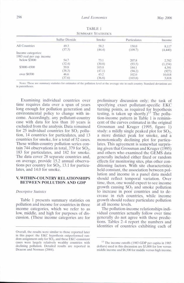
Examining individual countries overtime requires data over a span of yearslong enough for pollution generation andenvironmental policy to change with in-come. Accordingly, any pollutant-countrycase with data for less than 10 years isexcluded from the analysis. Data remainedfor 25 individual countries for SO2 pollu-tion, 14 countries for particulates. and 13countries for smoke, for a total of 32 cases.These within-country pollution series con-tain 744 observations in total, 379 for SO2.183 for particulates, and 182 for smoke.The data cover 28 separate countries and.on average, provide 15.2 annual observa-tions per country for SO2, 13.1 for particu-lates, and 14.0 for smoke.

V. WITHIN-COUNTRY RELATIONSHIPSBETWEEN POLLUTION AND GDP

Descriptive Statistics

Table 1 presents summary statistics onpollution and income for countries in threeincome categories, which we refer to aslow, middle, and high for purposes of dis-cussion. (These income categories are for

Overall, the results were similar to those reported lalerin Ihis paper: the EKC hypothesis outperformed ran-dom assignment only for SO2. and these EKC-consistentcases were largely relatively wealthy countries withdeclining pollution. Detailed results are reported inDeacon and Norman (2004),

preliminary discussion only; the task ofspecifying exact pollutant-specific EKCturning points, as required for hypothesistesting, is taken up shortly.)'^ The pollu-tion-income pattern in Table 1 is reminis-cent of the curves estimated in the originalGrossman and Kruger (1995. figure 1)study: a mildly single peaked plot for SO2,a more distinct peak for smoke, and amonotonieally declining plot for particu-lates. This agreement is somewhat surpris-ing given that Grossman and Kruger (1995)and others who examined the GEMS datagenerally included either fixed or randomeffects for monitoring sites, plus other con-ditioning factors. With site characteristicsheld constant, the association between pol-lution and income in a panel data mode!should reflect temporal variation. Overtime, then, one would expect to see incomegrowth causing SO2 and smoke pollutionto increase in poor countries and to de-crease in rich countries, while incomegrowth should reduce particulate pollutionat all income levels.

The pollution-income relationships indi-vidual countries actually follow over timegenerally do not agree with these predic-tions. Tables 2-4 report the numbers andidentities of countries exhibiting each of

" Vhfi income eutoffs (1983 GDP per capita in t985dollars) used in Ihis discussion are $3,800 for low versusmiddle income and $6,5(K} for middle versus high ineome.


TABLE 2THE SHAFH OF POLLUTION-GDP RELATIONSHIPS:

Sulfur Dioxide

Peak (invcrted-U)Mean GDP at peak

TroughMean GDP at trough

IncreasingCenter of GDP range

DecreasingCenter of GDP range

N

46,287

43,427

28,540

158,882

Countries

China, Ireland. Hong Kong, Italy

Chile. India, Poland, Portugal

Japan, Venezuela

Australia, Belgium. Brazil, Canada, UK.Egypt. Finland, West Germany. Iran, U,S.Israel, Netherlands, New Zealand, Spain, Thailand

the four possible shapes for pollution-income plots, plus summary statisties ontheir ineomes. Table 2 shows results forsulfur dioxide pollution, with 25 countriesavailable to examine. The most commonshape is decreasing (pollution falls with ris-ing income), which occurs in 15 countries.Most of the eountries in this group wouldbe classified as high income and the groupas a whole has above average income,which agrees with the EKC hypothesis. Thegroup does contain two anomalies, Egyptand Thailand, which are both poor. The re-maining 10 countries show no tendency toagree with the EKC hypothesis. Pollutionincreases with income in two countries,Japan and Venezuela, and neither is poor.A trough, which is never EKC-consistent,appears in four cases, exactly as often asthe inverted-U. While the inverted-U ap-pears four times, two of these are not EKC-eonsistent: China is too poor, and Italy toorieh, for their inverted-U patterns to agreewith EKC turning points in the literature.

It might be argued that countries expe-riencing little GDP growth over the sampleperiod should be given httle weight whenassessing the EKC's predictive power.Dropping the eight eountries that grewless than 20% between bottom and topincome tritiles, however, does not improvematters.''* The remaining countries still ex-hibit equal numbers of peaks and troughs,three each. Two of the three peaks, China

The eight are Australia, Brazil. India. Ireland, Israel,New Zealand, the Netherlands, and Ihe United Kingdom.

and Italy, are not consistent with the EKC.Japan and Venezuela with their increasingpollution-income patterns remain in thesample. The "deereasing" group is reducedby six, of which five are relatively well offand one is middle income. Overall, thepattern in Table 2 is largely preserved: theEKC-consistent cases for SO2 consist ofrich countries that reduced pollution astheir incomes increased.'"''

The descriptions of shapes in Table 2 arebased solely on comparisons of means,without requiring that the pollution meansin adjaeent tritiles be statistically distin-guishable from one another. This is appro-priate for the hypothesis testing carried outlater because these tests examine the fre-quencies of EKC-consistent patterns insamples of pollution-income plots, ratherthan testing for signifieant departures fromEKC-consistency in individual plots. Fordescriptive purposes, however, it is of inter-est to know which of the plot shapes inTable 2 are statistically distinct."* Restrict-ing attention to countries for which a /-test

• If one looks only at countries that grew more than50% between bottotii and top Iritiles (Egypt. HongKong, Iran, Japan, and Thailand) the fit to EKC pre-dictions actually seems worse. One country exhibits apeak and none exhibit troughs, an apparent improve-ment. However, one rich country (Japan) still displaysan increasing pollution-income relationship and theIhree countries with decreasing relationships are eitherpoor (Egypt and Thailand) or of middle income (Iran),

'" Our tests for statistically distinct pollution levels inadjacent tritiles proceed by comparing the means andstandard deviations ut ihe point estimates of pollution in


TABLE 3THE SHAPE OF POLLUTION-GDP RELATIONSHIPS: PARTICULATE.S

Partieulates

Peak (Inverted-L')Mean GDP at peak

TroughMean GDP at trough



N

26,231

64.320

111.324

5S,,S05

Countries

China, Finland

Belgium. India, Indonesia, IranMalaysia. PortugalDenmark

Australia, Brazil, Canada, Japan,ITiailand

indicates that the first tritile mean is sta-tistically different (at 10%) from the sec-ond tritile. and the second from the third,leaves only seven SO2 cases.'^ All are high-income countries for which SO:̂ declinesas income increases, hence all are EKC-consistent. When pollution means are sig-nificantly different for one pair of adjacenttritiles but not the other, a comparison oftwo points is possible. Both increasing anddecreasing plots, the only possible outcomeswith two data points, are EKC-consistentfor a middle income country, so sueh two-point comparisons are informative only forpoor and wealthy countries. Seven signifi-cant two-point comparisons are possiblefor SOi. Four of these agree with the EKCand three do not. For poor countries weobserve one significant increasing plot(India) and one decreasing plot (China),and for rich countries we observe two in-

each tritile, A referee correctly points out that two addi-tional sources of error are present in our tritile pollutionfigures: the sampling error that results front computingannual average pollulion levels from daily monitor-ing readings and the estimation error present in theregression equations used to form our within eounlrypollution series from Ihe moniloring site data. Incor-porating these sources of error into our analysis wouldrequire Information on the distributions of individualmonitoring sile observations, which are unavailable tous. The regression results used to form our within coun-try pollution series, Ineluding estimated standard errors,are available to the interested reader on request. Clearly,incorporating these additional sources of error wouldreduce the number of statistically significant pollution-income plots available to consider,

'̂ Tlie countries are Australia, Belgium, Canada,West Germany, Spain, the United Kingdom, and theUnited Stales.

creasing plots (Japan and Venezuela) andthree deereasing plots (Finland, Italy andNew Zealand). Overall, the only system-atic agreement with EKC predictionsamong statistieally significant cases is SO2reductions accompanying income growthin rich countries, and this agreement isevident only in three-point comparisons.

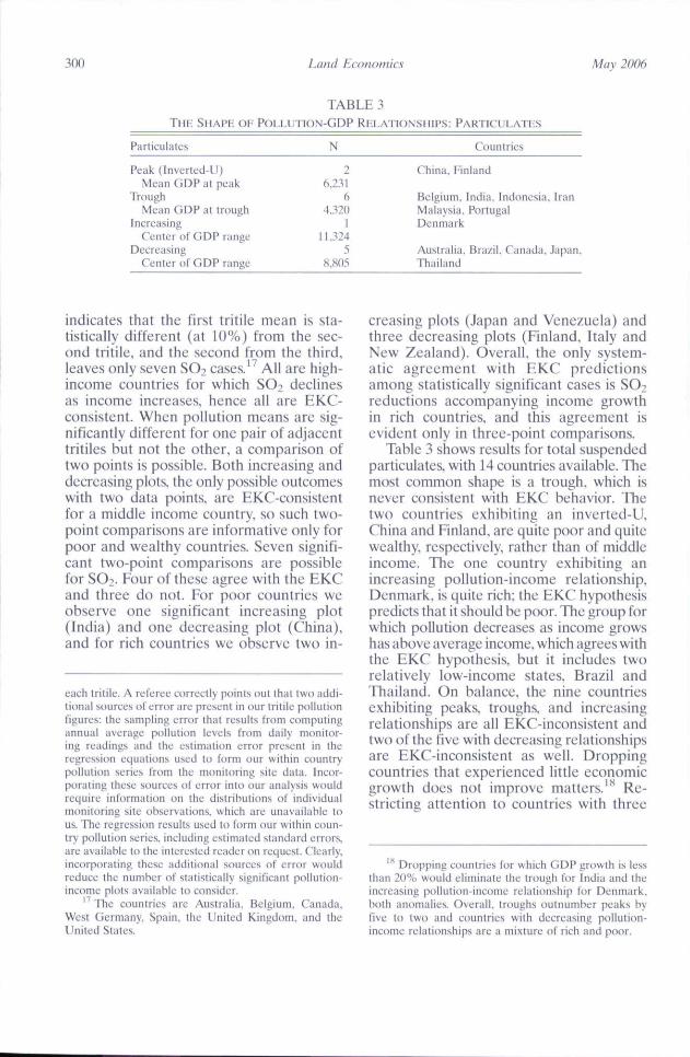
Table 3 shows results for total suspendedpartieulates, with 14 countries available, Tliemost common shape is a trough, which isnever consistent with EKC behavior. Thetwo countries exhibiting an inverted-U.China and Finland, are quite poor and quitewealthy, respectively, rather than of middleincome. The one country exhibiting anincreasing pollution-income relationship,Denmark, is quite rieh; the EKC hypothesispredicts that it should be poor. The group forwhich pollution decreases as income growshas above average ineome. which agrees withthe EKC hypothesis, but it includes tworelatively low-ineome states, Brazil andThailand, On balanee, the nine eountriesexhibiting peaks, troughs, and increasingrelationships are all EKC-inconsistent andtwo of the five with decreasing relationshipsare EKC-ineonsistent as well. Droppingcountries that experienced little eeonomiegrowth does not improve matters."^ Re-stricting attention to countries with three

Dropping countries for which GDP growth is lessthan 20% wouid eliminate the trough for India and theincreasing pollulion-income relationship for Denmark,bolh anomalies. Overall, troughs outnumber peaks byfive to two and countries with decreasing pollution-income relationships are a mixture of rich and poor.


TABLE 4THE SHAPE OF POLLUTION-GDP RELATIONSHIPS: SMOKE

Smoke

Peak (Invcrted-U)Mean GDP at peak

Trt)ughMean GDP al trough



N

34.408

35,798

29.L'i5

57.861

Counlries

Egypt. Poland. Venezuela

Beliiium, Chile, Iran

Denmark, Ireland

Brazil, Hong Kong. New Zealand.Spain. United Kingdom

Statistically distinct tritile pollution meansleaves us with two troughs, Malaysia andIndonesia, and one rich country with adeclining pollution-income plot. Canada.Three statistically significant two-pointcomparisons are possible and all involvewealthy countries: two of these plots aredecreasing (Australia and Belgium) andone is increasing (Denmark).

Results for smoke, presented in Table 4,also show no clear agreement with the EKChypothesis. There are as many troughs aspeaks, three eaeh. One of the three coun-tries exhibiting a peak, Egypt, is too poor tobe crossing an EKC turning point, based onestimates in the literature. The group forwhich pollution increases with output isrelatively wealthy, not poor as the EKCpredicts. Four of the five countries wherepollution decreases as income rises areindeed rich, which agrees with the EKChypothesis. Overall, however, the adher-ence to EKC predictions is poor at best.Dropping countries that grew less than20% would eliminate roughly equal num-bers of anomalies and EKC-consistentcases.''* There are no smoke cases forwhich all three tritile points are statisticallydistinct. There are six significant two-point

' This would eliminate the following countries:Brazil, Denmark, Ireland, New Zealand, and the UnitedKingdom, The two increasing cases in Table 4 are thusremoved. For the decreasing cases, two instances ofEKC agreement would be removed. New Zealand andthe United Kingdom, plus one case of disagreement,Brazil. The reduced set of comparisons would stiil showthree troughs, and the EKC-inconsistent peak, Egypt,would remain.

relationships. Contrary to EKC predic-tions, these cases show identical qualitativebehavior by rich and poor countries. Braziland Poland, both poor, have decreasingpollution-ineome plots, as do Belgium andthe UK, which are rich. Two countries dis-play significant increasing pollution-incomeplots: Chile, which is poor, and Denmark,which is rich.

Hypothesis Tests

The first null hypothesis examined is thatthe frequency of EKC-consistent ob-servations in the data is no different thanwould occur by chance. Other tests considerrelated hypotheses. The tritile data onpollution and income for a single country-pollutant case are treated as an observation.Each observation includes an income rangeand a shape for the pollution-income plot.Depending on where the income range liesrelative to the EKC turning point, the ob-servation is either qualitatively consistentor inconsistent with the EKC hypoth-esis. Accordingly, the frequency of EKC-consistent observations in the data ean becomputed. Of course, even randomly gen-erated data will agree qualitatively with theEKC hypothesis in some fraction of cases.Once the latter fraction has been deter-mined, the y^ distribution can be exploitedto test the null hypothesis stated above.

To judge EKC-consistency for eachcountry-pollutant case, EKC turning pointsfor each pollutant must be identified. This iscomplicated by the fact that the literaturereports a broad range of turning points foreach pollutant. Rather than impose con-


sensus where none exists, we specify upperand lower bounds for "the" EKC turningpoint for a given pollutant and adapt ourtesting proeedure aeeordingly. The boundsidentified for EKC turning points (GDP percapita in 19S5 dollars) are drawn from fiveEKC studies that have examined data onconcentrations for the air pollutants eon-sidered here."" Table 5 identifies the studiesand the point estimates for turning pointsreported by eaeh. The table also reports themean and standard deviation of these pointestimates for eaeh pollutant. For SO2 andsmoke the lower and upper bounds used inhypothesis tests are set at the mean pointestimate plus and minus one standard de-viation. For particulates. the standard devi-ation is so large that applying the sameprocedure would cause the income tritiledata for nearly half of the available ob-servations to fall entirely between the lowerand upper bound. As explained shortly,when the range of possible turning pointsencompasses the entire set of tritile obser-vations for a given eountry, the EKC'sprediction on pollution-ineome plots is rel-atively uninformative —only the U-shapeis ruled out."' To render our tests for thispollutant more informative, we arbitrarilyset the range for possible turning points atthe mean of the point estimates plus andminus $1,500." The lower and upperbounds used in hypothesis tests are thus:

Pollutant Lower Bound Upper Bound

T A B L E 5

E S T I M A T E S O F EKC T U R N I N G P O I N T S

(GDP Pl-R CAPITA IN 1985 $)

SO2PartieulatesSmoke

$3,012$4,140$4,855

$6,1S8$7,140$8,140

"̂ None of the studies examined interacts incomewith other variables, hence the turning point estimatesare meant lo apply uniformly to all countries.

Additionally, only Iwo turning point estimates areavailable for partieulates and bolh are from a single,early EKC study,

^̂ We cheeked the sensitivity of our central con-clusions on EKC consistency for particulates by re-computing our test statistics using the mean plus andminus one standard deviation, as reported in Table 5,These cheeks, deseribed more precisely later, revealedthat our cenlral conclusions are not sensitive to thischoice of turning point ranges for particulates.

Author

Panayotou (1997)Grossman and

Kruger (1995)Barrett and

Graddy (2()(H))Torras and

Boyee (1999)Shafik and

Bandyopatay (1992)MeanStd, Dev.Mean - 1 std. dev.Mean -1- 1 sid. dev.

SO2

4,1354,053

4.2025.1873,8903,3603,6708,30.54,6001,5883,0126,188

Partic,

H.OOO3,2805,6403,3382,3028,978

Smoke

6.151

8,0977,3924,350

6.4981.6424.8558.140

Tests for qualitative consistency with theEKC are adapted to this range as follows:A pollution-ineome plot is judged EKC-eonsistent if it is possible to draw a single-peaked curve through the plot, such that thecurve's peak lies within the range specifiedabove. Figure 2 illustrates how this criterionis applied. The income levels for lower andupper bounds on turning points are denotedTPi^ and TP,/. respectively. Let /,/, /,,-w, and/,// be country /*s lower, middle, and upperineome tritile values. If /,// < TPi_. theeountry is low ineome and EK.C-consistencyrequires an increasing pollution-incomeplot. In Figure 2 the income range for thiscase is illustrated by the bracketed set ofincome points labeled ' ' 1 , " and the term"increasing" below this set of points indi-cates the shape of EKC-eonsistent plots.Given this country's income range, only anincreasing pollution-income plot could bepart of a single-peaked curve whose peak liesbetween TP^ and TPH. If TP,i < I,L. thecountry is high ineome and its income rangeis illustrated by the plot labeled ease "2."EKC consistency requires a "decreasing"pollution-income plot. In the data we exam-ine, 35 ofthe 52 cases available fall into eithercase 1 or case 2.

The same eriterion for EKC-consisteney—that a single peaked curve with a peak be-tween TPi and TP^ can be drawn througha country's tritile points —is applied toeountries exhibiting a set of income points


Pollution

or

5a. [ • • • ]

Incr, deer., or invcited-U

inverted-U

5c. [ • t

Incr, deer,, or inVcrted-U

5d. I • • . 1

., deer., or itivertcd-U

TPL TPH GDP per capita

FIGURE 2EKC-CONSISTENT POLLUTION-INCOME PLOTS

that lies wholly or partially within therange TP/ to TP,^. which we refer to as therange of uncertainty. Consider the caselabeled "3" in Figure 2. Two of this coun-try's income observations lie below TPibut the third lies above it. EKC-consistencyclearly requires that the first two pollution-income points display an inereasing rela-tionship, but the third point, which lies inthe range of uncertainty, could be eitherabove or below the second. Accordingly,monotone '"increasing"- and "inverted-U"-shaped plots are EKC-consistent for case3. Similarly, case "4" shows a country forwhich two income observations lie aboveTP/i. but one lies below it. In this case,"decreasing" and "inverted-U" shapes areEKC-consistent. Cases 5a-5d cover the re-maining possibilities. In each of these

cases, the country's middle observation onincome, 1^- lies within the range of uncer-tainty for EKC turning points. "Inverted-U"- shaped plots are clearly EKC-consistentfor these cases. "Increasing" and "decreas-ing" pollution-income plots can also liealong inverted-U shaped curves peakingwithin the range of uncertainty, however.Thus, increasing, decreasing, and inverted-U pollution-income plots are all judgedEKC-consistent for such cases.

For hypothesis testing, it is necessaryto determine the proportion of cases thatwould be judged EKC-consistent with ran-domly generated pollution and incomedata. Two alternative specifications of ran-domness are considered. The first, termed"changes independent," postulates thatthe level of income gives no information


about the direction in which pollution willchange in response to a ehange in income.Regardless of whether income is low or highinitially, an increase in income is equallylikely to be associated with iticreased ordecreased pollution under this form of ran-domness. Because the probability of ob-serving no change in pollution is virtuallyzero given the level of resolution in the dataused here, the possibility of no change inpollution is ruled out. With three data points,this process implies a one-fourth probabilityfor eaeh of the four possible shapes.̂ "*

The second version, called "levels inde-pendent," postulates that a country's pol-lution level is independent of its income.In this case, the pollution values in a givenpollution-income plot are three pollutiondraws from the same distribution. Labelthe pollution levels in these draws X, Y,and Z, and assume X < Y < Z. If X isdrawn when ineome is low, Z when incomeis middle, and Y when income is high,the resulting pollution-ineome plot is aninverted-U. The shape is also an inverted-U, however, if Y is drawn when incomeis low, Z when ineome is middle, and Xwhen income is high. In total there are sixdifferent orderings for X, Y, and Z so theprobability of drawing an inverted-U isone-third. A symmetric argument demon-strates that the probability of drawing atrough under this set of assumptions is alsoone-third. Similar reasoning shows that

the probabilities of monotone increasingor monotone deereasing pollution-incomeplots are one-sixth each with this proeess.

The first test examines a simple null hy-pothesis: the overall number of EKC-eonsis-tent plots observed in the data is no differentthan would occur if the data were randomlygenerated. The test requires the total numbersof EKC-eonsistent and EKC-inconsistentplots expeeted under random assignment,denoted C« and Ni^. respeetively, and thenumbers observed in the data, denoted Coand Nr). When computing the number ofEKC-eonsistent plots under random assign-ment, the known proportion of observationsin each ofthe ineome categories (Cases 1,2,3,4, 5a-5d in Figure 2) is imposed. For exam-ple, under changes independent randomnesswe specify that one-fourth ofthe observationsfor Case 1 (low ineome) eountries take oneach of the four possible shapes, and sim-ilarly for other income categories.

The test statistic is

- CoY No)'

which follows the x~ distribution under thenull hypothesis. With only two outeomes toeonsider, consistent vs. inconsistent, thereis one degree of freedom. Applying this testseparately to eaeh of the three pollutantsand using the two different versions of ran-domness yields the following results:

Ho' EKC-consistency observed with same frequency as with random dataH^: H() is false.

Changes Independent Levels Independent

% EKC Consistent % EKC-Consistent

Pollutant Observed Random y' (1) Prob, Observed Random y (I) Prob.

SO2ParticulatesSmoke

60%21%.38%

38%34%42%

5,140,980,0s

2.3%32%78%

60%21%38%

31%27%36%

9.550.250,37

0.20%62%85%

"̂' To sec this, plot the three data points with pollutionon the vertical axis and income on the horizontal axis.Given Ihe first data point, pollution in the second will beabove the first with probability (1,5, and pollution in thethird will be above the second with probability 0,5. Hence.

the probability of a monotone inereasing plot with thisform of randomness is 0,25. Similarly, the probability ofa monotone decreasing plot is also 0.2.'i, Using the samereasoning, it is easy to show that the probabilities ofsingle-peaked and single-troughed plots are 0.25 as well.

82(2) Deacon and Norman: Kuznets Curve and How Cotmtries Behave 305

The first two columns of numbers show,respeetively, the percentages of EKC-consistent cells observed in the data andunder the changes independent version ofrandomness- Thus, the percentage ob-served to be EKC-consistent in the dataranges from 21% for particulates to 60%for SO2; EKC-consistent percentages withehanges-independent random data rangefrom 34% to 42%. The next two columnsshow the /^ statistics and the probabilityof observing the fraction consistent in thedata under random assignment. The lastfour columns of numbers report corre-sponding statisties for the levels indepen-dent form of randomness.

For particulates and smoke, the levelsof EKCT-consistency observed in the datacould easily have occurred by chanceunder either version of randomness. Forparticulates, both forms of randomnessactually produce more EKC consistentcases than occur in the data. A sensitivitycheek reveals that this finding is not sen-sitive to an alternative choice of upper andlower bounds for EKC turning points.*̂ "̂This is unsurprising in light of the f'act thateight of the 14 particulate eases follow a U-shaped pattern, which is EKC inconsistentregardless of the turning point. For SO2.however, the data are significantly morecompatible with the EKC hypothesis thaneither version of randomness would yield.As discussed below, however, this agree-ment is of a very specialized *̂

•̂* The test was re-computing using $2,302 and $8,978as upper and lower bounds, whieh correspond to themean plus and minus one standard deviation of turningpoint estimates reported in Table 5, With ihese boundsthe tesl statistics revealed that the probability of findingthe observed degree of EKC consistency in random datais 78% with changes independent randomness and 84%with levels independent randomness.

" One might naturally consider a different proce-dure: test the null of random assignment against the al-ternative of EKC-consistency using a likelihood ratiotest. This strategy would not be informative, however,EKC theory, strictly interpreted, predicts that certainpatterns actually observed in the data are not possible,e,g.. troughs, so the sample would have zero likelihoodunder the EKC hypothesis. Specifying a stoehasiic vari-ant of the EKC theory is not something we have attempted.

The preceding tests only examine the"overall" predictive power the EKC hy-pothesis: Is the proportion of cells found tobe EKC-consistent greater than wouldoccur by chance? One might also wonderhow well the EKC hypothesis predicts theshapes of pollution-income relationshipsfor individual income categories. This is ofinterest because the EKC's predictive per-formance seems to be different for differentincome categories. To address this question,use the superscript / = 1..J to denoteincome categories. Then let C;̂ and N^denote the number of EKC-consistent andinconsistent cells expected in income cate-gory / with random assignment and let C^and /V/, denote the number of EKC-consistent and inconsistent cases in incomecategory/ in the observed data. Under thenull hypothesis that C^= C/^for all y, wehave the y~ statistic:

+•

This statistic assigns significance to depar-tures from randomness within individualincome categories, while the earlier test onlylooked at overall performance across all in-come categories. The test considers 2J fre-quencies, hence there are 2J - I degrees offreedom. In praetice, certain income catego-ries have no observations for some pollu-tants, so degrees of freedom differ from onetest to another. As before, the known pro-portions of observations in various incomecategories are imposed when computing thefrequencies with random data. Performingthis test separately for each of the three pol-lutants yields the following results:

Ho- EKC-consistency in income categoriesobserved with same frequency as withrandom data

H^: Ho is false.

Pollutant

ChangesIndependent

y^ (d.f.) Prob,

LevelsIndependent

(d.f.) Prob.

SO2 37.35Particulates 9.33Smoke 5.44

<0.OI% 56.74 <0.(H'23% [n.8O 16%61% 5.90 .55%


Again, the SO2 results are highly con-sistent with the EKC hypothesis but thepatterns for particulates and smoke couldeasily have arisen by chance.^^ The in-creased significance for sulfur dioxide re-sults from the fact that a very highproportion of cases in one income group,the high ineome category, are EKC-con-sistent. This pattern was, of course, evidentin the deseriptive statisties.

The last hypothesis examined considerswhether the plot shapes and incomecategories observed in the data exhibitany non-randomness at all. This involvesignoring EKC-eonsistency or ineonsisteneyand simply testing whether the numbersof observations falling into the various"plot shape/income category" cells differsfrom what would occur with randomdata. While the SO2 patterns are knownto be non-random, it is of interest to checkfor non-randomness for the other twopollutants. Examining frequeneies in allpossible eells seems exeessively detailed inlight of the numbers of observations avail-able. To simplify, the number of ineomegroups is reduced to three by eombiningcases 3, 4, and 5a-5d into a single "middle-income" group. There remain 12 possiblecombinations of plot shapes and incomecategories. A finding that the frequen-cies of observations in eaeh differ fromwhat random data would produce wouldnot indicate that the EKC has predic-tive power, of course, because there aremany non-random assignments and EKC-consistent assignments are only a subsetof these.

Let the superscript k = 1...12 index thecells (four shapes and three combinedincome categories) and let Eo and £«denote the numbers of observations occur-ring in cell k in the data and under ran-

domness, respectively. The appropriatetest statistic is

which follows a y^ (II) distribution. Re-sults for the three pollutants are

Ho: Observed cell frequencies equal fre-quencies wiih ramiom data

H^: HQ is false.

Pollutant y_

ChangesIndependent

11) Prob.

LevelsIndependent

) ^ (11) Prob.

SO2 26.71 <0.0t% 45.29 <0.01%Particulates 10.00 53% 10.50 49%Smoke 4.60 95% 7.70 74%

Only sulfur dioxide can be regardedas non-random; the observed pattern ofineome ranges and poUution-ineome-plotsfor particulates and smoke are not sig-nificantly different than what one wouldget by rolling a 12 sided, appropriatelyweighted die.^''

Looking aeross all three pollutants andconsidering the detailed criteria in Figure 1,the EKC fares poorly as a predictive prop-osition. In total, 23 of the 52 availableobservations are eonsistent with the EKC,while 29 are ineonsistent. The inverted-Uoeeurs nine times in the data while a U-shape, which is never EKC-consistent, oc-curs 13 times. Five of the 52 cases exhibita positive pollution-income relationship,but none of these are low-income eountries.The one bright spot for EKC-consistencyis the frequency with which high incomecountries reduced their pollution as incomegrew. These eases account for 15 of the 23EKC-consistent cases for all three pollutants

Performing Ihe lest for particulates using thealternative bounds for turning points revealed that theobserved EKC consistency in the data eould easily havearisen by chanee, with 74% probability for changesindependent randomness and with 64% probability forlevels independent randomness.

' The last set of tests was examined for robustnessto alternative ways of defining income groups based on1983 income levels. Results did not depend on the choiceof income culoffs.


combined, and for 11 of the 14 EKC-consistent observations for SO2.

Discussion and Extensions

Our findings agree with List and Gal-let's (1999) observation (from individualU.S. states) that pollution-income relation-ships tend to vary across political units.When they allowed for state-specific inter-cept and income slope terms in a paneldata model, they found a wide range ofSO2 emission turning points, from $2,989{Rhode Island) to $69,047 (Texas) using aquadratic specification, and from $6,428(Arizona) to $95,703 (Texas) with a cubicspecification. Only a small fraction of theturning points obtained from these state-specific EKCs were within one standarddeviation of the turning points they ob-tained by estimating a "traditional" EKCmodel, allowing only for state-specificintercepts. This led them to conclude thata "one size fits all" approaeh may result inbias. List and Gallet's (1999) results couldbe more thoroughly compared to ours bydetermining the shapes of state-specificpollution-income relationships over theincome ranges actually observed in theirdatasets. This would no doubt reveal thatsome states exhibit deereasing, others in-creasing, still others possibly u-shaped,pollution-income relationships.

In the dataset we examine. EKC-consistent behavior within countries islargely confined to high-income nations.This is noteworthy because high-incomecountries are overrepresented in the GEMSdataset. Countries with 1983 per capita GDPgreater than $7,000 represent exactly one-half of all the country-pollutant cases inthe GEMS data we examine, but only22% of the 144 countries in the PennWorld Tables. Countries with incomes be-low $3,500 eomprise 21% of the country-pollutant pairs in our sample, but 58% ofobservations in the Penn World Tables.The fact that richer countries are over-represented, together with the observationthat EKC-consistent behavior is largelyconfined to richer countries, implies thatthe cards are stacked in favor of accepting

the EKC hypothesis as a general prop-osition in the GEMS dataset. This is un-fortunate because a primary aim of EKCanalysis is to predict the environmentalimplications of growth in poorer countries,thai is, the group that is underrepresentedand for which the EKC predicts poorly.

The potential role of European Union(EU) policy also merits discussion. Ten ofthe 28 countries examined here were EUmembers during the sample period, in-cluding three that joined during thisperiod. This is potentially signifieant be-cause EU Direetive 80/779/EEC requiredboth EU members and prospective mem-bers to harmonize air quality standards forSO2 and particulates in urban areas. It alsodirected EU members to uphold domesticlaws consistent with the "environmentalacquis," the body of laws and standardsagreed to by the union. The compliancedate, 1983. falls roughly in the middle ofthe sample period."^ Contrary to the EKChypothesis, this and other EU environ-mental directives required a single policyresponse of all members regardless of in-come level or growth. In addition, becausethe environmental acquis applied to pro-spective as well as existing members, adesire for EU membership may have moti-vated more cleanup than would otherwisehave occurred among countries such asSpain and Portugal, which joined duringthe sample period and after the initialdirective was established. Additionally, theEU subsidized the pollution control ofpoorer member states, including Ireland,Portugal and Spain, so for these states EUpolicy increased the benefits of pollutioncontrol (by tying them to the other benefitsof membership) while simultaneously re-ducing the eosts.^"

It is instructive to reconsider the de-scriptive results for Ireland, Spain, and

The regulation was revised by Directives 89/427/EEC and 91/692/EBC. which also fall witbin the sampleperiod. Information on EU poliey was taken from Kraus(1997),

^̂ The EU Structural Fund and Ihe EU CohesionFund adminislered these subsidies; Hansen and Ras-mussen (2001),


Portugal in this light. Ireland appears in thesample for smoke and for SOi. Ireland'ssmoke, which was not covered by EU reg-ulations, rose steadily with income, nearlydoubling between first and third tritiles.Ireland's SO2. which was covered by EUpolicy, exhibits an inverted-U relationship,declining sharply in the final tritile. Spain,a prospective member in 1980, also reportsdata for smoke and SO2. Both pollutantsfell sharply in Spain between the first andthird tritiles of observations and, becauseSpain is relatively rich, this is eonsistentwith the EKC hypothesis. Spain's mostdramatie reductions were for SO2. how-ever, which was covered by the EU direc-tive and for which Spain reeeived EUsubsidies, and these reductions were dee-pest after the EU policy went into effect,Portugal reports data for SO2 and particu-lates. both of which were regulated by theEU. Portugal's plot for both pollutants is atrough, whieh reached bottom the mid-1980s and jumped sharply in 1989-1992,Without claiming that EIJ polieies wereresponsible for any of the EKC-eonsistenteases found in the data, these instancesillustrate the difficulty of separating the airquality effeets of EU polieies, whieh arenot part of the EKC story, from theincome-driven processes emphasized inthe EKC literature.'"

One advantage of the within-eountryapproaeh —minimizing the influence of un-observed heterogeneity —is lost if a coun-try's attributes ehange. A country's systemof government is an attribute that some-times shifts, and it is potentially importantbecause democratic and non-democraticgovernments may well provide differentlevels of pollution eontrol. Because ineomeand political institutions are highly corre-lated, failure to control for political changemight bias the shapes of estimated pollu-

•"' These policy responses would conform to theEKC story if Ihe LLI were trealed empirically as a singleslate, bul this has not been the practice in the EKCliterature, DeBruyn (1997) also addresses the potcnlialrole of EU policy for pollution in member countries.

tion income relationships."" In addition,poliey processes driven by income growthmay operate differently in demoeraeiesand autocraeies and give rise to differentEKC responses."''̂

The importance of this considerationwas assessed by examining each country's"polity score," a variable indieating thepresenee of demoeratie attributes such asconstraints on the chief executive, compe-tition for political offiee, and openness topolitical participation, versus autocraticattributes (see Marshall and Jaggers 20()0).Polity scores can range from 0, indieatingautocracy, to 1, indicating demoeraey.Countries experiencing substantial politiealchange during the sample period were firstidentified and dropped from the sample.Tests of the EKC's predietive power werethen earried out separately for democraciesand autocracies. "Politieal changers" weredefined to be countries whose polity scoreschanged by at least 0.3 during the sampleperiod." Four countries met this criterion:Brazil, Poland, Spain, and TTiailand. Non-ehangers were classified as autocracies iftheir mean polity scores were .35 or belowand as demoeraeies if their polity seoresaveraged 0.9 or above.̂ "̂

'̂ While various authors have ineluded politicalindicators ;imong Ihe independent variables in reducedform EKC models, they have not interacted Ihese termswith income. In effect, pollution was allowed to be higheror lower under dictatorship th;in democracy, but theshape of the income-pollution curve is the same for both,

-" See Lopez and Mitra (21)00), List and Slurm (2004)find thai changes political competition within democra-cies can cause changes in the stringency tif environmentalpolicy. They use term limits as a vehicle for representingvariations in political competition: competition is re-duced during an elected politician's final term. Ourexamination of political ehiinge looks at shifts betweenaulocracy and democracy, but does not consider electoralrules and Ihc timing of governmental leaders' terms ofoffiee wilhin democracies at this level of detail,

•'•̂ This cutoff resulted in a fairly sharp distinction. Ofcountries classified as non-changers, only two experi-enced a change in polity of as much as 0,2 and changes inthe remaining non-changers were all 0,1 or less.

'"* Five eountries met the autocracy criterion: China,Chile. Egypt, Indonesia, and Iran. Seventeen met thedemocracy criterion: Australia, Belgium. Canada. Den-mark. Finland. India, Ireland, Israel, Italy. Japan, NewZealand. Netherlands. Portugal, the United Kingdom,


Because the results do not differ mark-edly from those reported earlier, they areonly summarized here and details areavailable on request. For particulates andsmoke, the /^ statistics that examine EKC-consistency in individual income categoriesindicate that the probability of getting anequal or better match to EKC predictions inrandotn data is 0.60 for autocracies and 0.24for democracies. The SO2 results are moreinteresting. For autocracies, agreement withEKC predictions is substantially worse thanwould occur by chance, so the EKC hypoth-esis elearly is not supported. For democra-cies, agreement with EKC predietions isvery strong, but this agreement is domi-nated by one now-familiar pattern —wealthy countries that reduced pollutionas their incomes increased. Indeed, 10 ofthe 11 instances of EKC-consistent behav-ior among democracies are of this type. Theonly EKC-consistent demoeraey showingdifferent behavior is Ireland, a middle-income country displaying an inverted-U/̂ ^^The consideration of political attributes thusallows the set of cases exhibiting EKC-consistent behavior to be narrowed fur-ther, to wealthy democracies that reducedSO2 pollution.

Changes in pollution may result fromfactors that change over time but areunrelated to income, such as better infor-mation on health risks and improvementsin pollution control technology. Panel dataEKC models often include a trend variableor year dummies to account lor temporalfactors that are common to all countries. Insuch models, the EKC hypothesis amountsto an inverted-U relationship betweenincome and the variation in pollution thatis not explained by trend-related factors.The hypothesis tests performed earlier did

the United States. Venezuela, and West Germany. Twocountries were dropped from this part of the analysis:Hong Kong because no polity score is reported andMalaysia because ils polity score (U.7) fell between thebounds sel for autocracy and democracy,

" A very slight change in Ireland's lower incometritile would have moved it into the high incomecategory, in which case its inverled-U would have beenEKC-inconsistent.

not eontrol for purely trend-related influ-ences on pollution and this might haveaffected the data's conformance to EKCpredictions. To examine this possibility,purely time-related movements in eaehpollutant, common to all countries, wereestimated using panel data EKC modelsfor each pollutant. The models includedfixed effects for years and countries, thirdorder polynomials in per capita GDP andeaeh observation's polity score as indepen-dent variables. The yearly fixed effectsrepresent the time-related movements inpollution that remain after controlling formovements in income and politics. Thesetime-related movements were removedfrom each pollution series by subtractingthe yearly f'ixed effects. Tests for qualita-tive EKC-eonsistency were then recom-puted with these detrended pollution data.

Using detrended pollution data did notimprove the EKC's predictive perfor-mance. For smoke, with 13 cases toexamine, the number classified as EKC-consistent dropped from five to four. ForSO2, with 25 cases to eonsider. the numberof EKC-consistent cases fell from 15 to 14.For particulates, with 14 available cases,the number agreeing with the EKC de-clined from three to two. The probabihtiesthat the EKC-consisteney observed in thedata could have oecurred by chanceincreased commensurately.

VI. REDUCTIONS IN SO2: DECLININGTREND OR INCOME EEFECT?

The one EKC-consistent pattern in thedata is a strong tendency for wealthiereountries to reduce SO2 pollution as theirineomes grow. Pollution and income wereboth trended during the 1970s and 1980s,however, so the pollution reduction couldalso be attributed to any other trendeddeterminant. One such determinant is ashift in preferences toward environmentalprotection, caused perhaps by better infor-mation on environmental risks and improve-

^'^ Detailed results, including parameter estimatesfor the panel data model, are available on request.


ments in pollution eontrol technology. High-ly publicized oil spills and eiaims regardingthe effects of pesticides and industrialchemicals in the late 196(}s were followed inthe United States and other wealthycountries by the first observance of EarthDay, the 1972 UN. Conference on theHuman Environment, and by legislation tocontrol air and water pollution, proteet en-dangered species, and control land usechanges."'̂ These events happened abruptly,suggesting a shift in public preferences, butthe goal could only be achieved gradually ascontrol technology developed and politicalhurdles were overcome. This line of argu-ment suggests a different explanation for thedownward trend in SO2 and other pollutantsevident in the 197()s and 1980s. Perhaps itwas part of a transition from an old "lowenvironmental awareness equilibrium" to anew equilibrium where environmental pro-teetion was high on the public agenda. Whilethis alternative story does not stress incomegrowth as a key faetor in reducing pollu-tion, higher-income countries may well haveadopted more ambitious environmentalgoals and achieved them more rapidly. Thepower of this explanation, which attributespollution reductions to unobserved trendedfactors, versus the income-driven EKC ex-planation for SO2 reductions, is examined inwhat follows.-̂ ^

The within-country time series datawere used to estimate simple models, onemodel for eaeh eountry in the SO2 dataset,in which SO2 is a function of a trend. Theestimated trends were then examined tosee if SO2 reductions were more rapid inwealthier eountries. To check the power ofthe EKC model, a third order polynomialin per capita GDP was then added to eaeh

of these within-country models and thecoefficients were tested for joint signifi-canee. Because the "trend seenario" is asimpler explanation for SO2 reductionsthan the EKC, we apply Occam's razor andadopt it as the null hypothesis in subse-quent testing. Estimating models withtwo trended series, ineome and pollution,raises econometrie issues that are ad-dressed as they arise.

Table 6 gives results for the 25 countriesin the SO2 dataset. Pollution was expressedin logs to ease eomparisons of trendsaeross countries. The estimated trends arereported in eolumn (1). All of the signif-icant trends are negative and all but one ofthese oeeur in wealthy countries. Thecorrelation between the trend eoefficientsand mean per eapita GDP is -0.48, which issignificant at 1%. Pollution reduction wastherefore more rapid in wealthier coun-tries.'' GDP terms were then added andthe models were re-estimated by OLS. Asindicated in column (2), the GDP termswere jointly significant at 5% (using an F-test) in 10 of the 25 eases.'̂ " The time trendpresumably eaptures part of the effeet ofincome growth beeause income generallyrose in most of these 25 eountries, leavingincome terms to explain only deviationsaround that trend. While ineluding incomeand a trend together makes it diffieult toseparate the effeet of ineome from a puretrend effect, this is common practice inEKC researeh.

Before interpreting the GDP coeffi-cients, a number of econometrie issuesmust be addressed. Income is widely be-lieved to follow a unit root process andpollution may follow a unit root as well.When a regressor follows a unit root pro-cess its coefficient is not normally distrib-uted, even in large samples, and the usual

"'' See Portney (1990,) for a review of pre- and post-1970 air pollution poliey in the U.S, According toPortney (1990, 48-51,) U,S. emissions of particulatesdropped rapidly after iy70 and sulfur dioxide emissions,which had peaked in 1970. fell steadily thereafter.

• The idea that observed abatement in the devel-oped countries may be time related ralher than aproduct of income growth is noted in Stern andCommon (2001); see also Stern (2002, 201).

The correlation between trends and mean polilyscores is -0,43, indicating more rapid cleanup indemocracies.

""̂ Per capita GDP terms were jointly significant at10% in four other countries: Belgium, Canada, Finland,and Italy. Adding the GDP terms naturally changed theestimated trends. The trend eoefficients in eolumn (1)are those estimated from a model without GDP terms.


w i

^ oi Z

CO << Q- Qt- z to

O a:P O

>- iUQ! Q.h- £1-

I LU

Q. ,5

o y

— T r- iri — —

00 o M 00o O ^ t M r

sc — 'S-, >O

E E E

O (N OC

d d —

o aOC 3^ 0000 " r~̂

I I

C f r n Q Q ^ O C X r , rN r n ^ D r j t N / , r J r J r ; S w j * C^ ^ ^ o O O O O O O — O O •—' O O 1—' O O 1—I O •—• O Ooddddddcoddddddoddcdodoc

I I I I I I I I I I I I I I I I I I

< m en

cuc

cop

u3

,s*


critical values for hypothesis tests do notapply. More disturbing, if both variablesfollow stochastic trends a significant esti-mated relationship between the two maybe spurious. The latter concern is moot,of course, if income terms are statisticallyinsignifieant. To check for unit roots,augmented Dickey-Fuller tests were per-formed on income and pollution for the 10countries exhibiting jointly significant in-come terms.• '̂ The hypothesis of a unit rootin ineome could not be rejected (at 5%) forany country and a unit root in pollutioncould be rejected only for China.

Having unit root series on both sides ofan estimated equation is not a problem ifthe two are cointegrated, that is, if theyfollow the same stochastic trend. Cointe-gration was indicated for all nine eountriesdisplaying unit roots in both pollution andineome.'*^ Serial correlation is another po-tential concern, so Durbin-Watson testswere performed on the OLS residuals ofthese nine models. In al! eases, the statistieseither indicated rejeetion of the hypothesisof first-order serial correlation at 5% orfell into the indeterminate range. Accord-ingly, the OLS income coeffieients for thesemodels, reported in columns (3)-(5), areinterpreted as usual. The remaining case,China, exhibited a unit root in income butnot in pollution."^^ First-differeneing China'sincome and pollution twice yielded serieswith unit roots. Further, the hypothesis ofcointegration could not be rejected for the

Dickey-Fuller tests were performed on incomelevels only, and nol separately on income squared andincome cubed. Perman and Slern (2003) note that loworder polynomials retain the unit root property whenIhe untransformed variable follows a unit root. As wefocus here on within-eounlry relationships we do nottests for unit roots in a panel, as in Jewell et al, (2003),Im, Pesaren. and Shin (2003) and Im, Lee, and Tieslau(2005),

"^ The null hypothesis, that the residuals follow aunit root, was rejected al 1% or better in all cases,

''•' It is not possible for an independent variable tofollow a unit root process while the dependeni variabledoes not. However, given the short time series weobserve and the relatively low power of unit root tests,we are not inclined to regard this as eompelling evidenceof a specification problem.

double-differenced data and residualsfrom the model with double-differeneeddata did not display positive first-orderserial eorrelation. For China, then. Table 6reports OLS results from the mode! esti-mated on double-differenced data,'*'*

For the 10 eountries with jointly signif-icant income terms, the GDP coeffieientswere used to determine turning points forpollution-income relationships. Becausethese models inelude third-order polyno-mials in GDP, they typieally have twoturning points. Columns (6) and (7) reportthe GDP values of left and right turningpoints and indieate whether a given turn-ing point is a max (peak) or a min (trough).To allow tests for EKC-eonsistency, eachcountry's income range is reported in col-umns (8) and (9) and its income eategory,as defined in Figure 1. is reported in eol-umn (10), Column (11) reports the shapeof each country's pollution-income fune-tion over the range of income observed inthe data. Next, we indicate whether or nota country's estimated pollution-ineomefunction is EKC-consistent.

Brazil provides one clear ease of EKC-consistent behavior. Its ineome range liesentirely within the upper and lower boundson SO2 turning points, so increasing, de-creasing, or single-peaked functions wouldbe eonsistent with the EKC hypothesis.Brazil's estimated pollution-ineome func-tion is peaked, and hence is EKC-consistent.Relaxing the EKC-consistency eriterionslightly, Iran eould also be regarded asEKC-consistent. Iran's income range alsolies whhin the upper and lower bounds forEKC turning points, so inereasing, decreas-ing, and peaked shapes are EKC-consistent.Iran's pollution-income function actuallyshows a trough at $4,242 and a peak at$4,886. but there is only one data pointbetween these two values and the function isnearly flat over this range. Iran's pollution-income function is thus "nearly downwardsloping," and hence is nearly eonsistent withthe EKC hypothesis.

•" Estimating China's model with undiffercnced dataproduced very similar income coeffieients.


The remaining eight pollution-ineomerelationships are EKC-inconsistent. China,a low-income country, has a peak followedby a trough and both are at ineome levelswell below our range for EKC turningpoints."*'' Thailand, also low-income, has atrough shaped plot over its income rangeand 13 of its 15 data points are in a regionwhere predieted pollution declines as in-come increases, eontrary to the EKChypothesis. Hong Kong's income rangecrosses the upper bound for SO2 turningpoints, so a peaked or decreasing pollution-income curve would be EKC-consistent.Hong Kong"s plot actually increases mono-tonically over the data range observed.

The five remaining cases are all high-income countries. Japan and Venezuelahave peaked pollution-income plots overranges of observed data, with peaks occur-ring at income levels well above levelsreported in the literature, $12,738 and$8,153, respectively. Most of the datapoints observed for these countries (18out of 21 for Japan and 15 out of 16 forVenezuela) are in a range where predictedpollution increases as income increases,contrary to EKC predictions for a richcountry. Israel is another high-incomecountry for which pollution increases withincome. The Netherlands exhibits a dis-tinct trough over the data range. Thiswould not be troubling if most of the datawere on the downward sloping region,where pollution decreases as income rises.In actuality, 12 of the 15 observations forthe Netherlands are in a range where in-come growth leads to higher pollution. Theremaining eountry. New Zealand, exhibitsa trough followed by a peak, with both oc-curring at income levels well above peaksreported in the EKC Uterature.^'' On bal-ance, when one allows for purely trenddriven factors to explain within-countrypollution, the additional explanatory power

of income is typically not significant and,where significant, its effect is not consistentwith the EKC hypothesis."*^

VII. CONCLUSIONS

Looking within individual countries, attheir experiences over time with eeonomicgrowth and changes in pollution, and al-lowing each country lo have a differingturning point, we find only a highly spe-cialized form of agreement with EKCpredictions. Relatively wealthy democraciescontrolled their SO2 pollution as their in-comes increased, which is consistent withthe EKC hypothesis. The remaining EKCpredictions, that is, pollution increasingmonotonically with income in poor coun-tries, and middle-income countries follow-ing an inverted-U path, are not observed forSO2. For sn^oke and particulate pollution,instances of agreement with EKC behaviorare not observed with any greater frequencythan chance would dictate.

The SO2 reductions that occurred in richeountries, while consistent with the EK.Cstory, are also consistent with any otherforce causing a secular decline in pollutionduring the 1970s and 1980s. One explana-tion was offered in the text, but there maybe others. Once the effect of purelytrended factors is accounted for. incomegrowth has no consistent predictive powerfor the patterns of changes in pollutionexperienced by individual countries.

The aim here was not to develop aframework for understanding why pollu-tion behaves as it does in individual coun-tries. This is obviously an important task,but one that is well outside the scope of thepresent analysis. Rather, the intent was tosee if the EKC hypothesis gives reliablequalitative predictions about the way pol-lution behaves within individital cotintriesthat experience economic growth. Based

"''' The predieted pollution-ineome plot for China isrelatively flat, however, so income's role in determiningpollution is very minor,

•*" In New Zealand's case, the effeet of ineome onpredicted pollution is very slight.

•*' Perman and Stern (2003) reach the same generaleonclusion. Our results also agree with Stern andCommon's (2001) conclusion that reductions in sulfuremissions are more time driven Ihan due to incomegrowl h.


on an examination of the data presentlyavailable, using robust empirical methodsto test what the EKC prediets, we find thatmost of the observed patterns eould easilyhave occurred by chance. In the limited setof circumstances where the EKC's predie-tions are upheld, the observed behaviorhas a simpler explanation.

References

Andreoni. Jatnes, and Arik Levinson. 2001. "TheSimple Analytics of the Environmenlai Kuz-nefs Curve." Journal of Public Economics 80(2): 269-86,

Antweiler, Werner. Brian R. Copeland, and M.Scott Taylor, 2001, "Is Free Trade Good for theEnvirontiient?" American Economic Review91 (4): 877-908.

Barbier, Edward B. 2(X)I. "The Economics of Trop-ical Deforestation and Land Use: An Introduc-tion to the Special Issue." Land Economics 11(May): L^5-71.

Barrett, Scott, and Kathryn Graddy. 2000, "Free-dom, Growth, and the Environment" Environ-ment and Development Economics .'i(4): 433-56,

Brock, William, and Scott Taylor. 2004, "TheGreen Solow Model," NBER 10557. Workingpaper, Cambridge, Mass,: National Bureau ofEconomic Research.

Carson. Richard T . Y, Jeon, and D,R. McCubbin.1997. "The Relationship Between Air Pollu-tion and Income: US Data." Environment andDevetopment Economics 2 (4): 433-50.

Cole. Matthew A. 2003. "Development, Trade,and Ihe Environment: How Robust is the En-vironmental Kuznets Curve?" Environmentand Development Economics 8 (4): 557-80.

Coondoo. D., and S. Dinda. 2002, "Causalitybetween Income and Emissions: A CountryGroup-Specific Econometric Analysis." Eco-logical Economics 40 (3): 351-67,

Copeland. Brian R,. and M. Scott Taylor. 2003.Trade and the Environment: Theory and Evi-dence. Princeton, N.J,: Princeton University Press.

Deacon, Robert T , and Catherine S. Norman.2004. "Is the Environmental Kuznets Curve anEmpirical Regularity?" UCSB Working Paper22-03, Department of Economics, Universityof California, Santa Barbara.

De Bruyn, Sander M. 1997. "Explaining the Envi-ronmental Kuznets Curve: Structural Changeand International Agreements in ReducingSulphur Emissions." Environment and Devel-opment Economics 2 (4): 485-503.

Grossman, Gene, and Alan B Krueger, 1993."Environmental Impacts of a North AmericanFree Trade Agreement," In The Mexico-US.Free Trade Agreement, ed, Peler Garbcr.Cambridge, Mass.: M.I.T Press,

. 1995. "Economic Growth and theEnvironment," Quarterly Journal of Econom-ics 112 (2): 353-78.

Hansen, Dinne, and Michael Rasmussen, eds.2001, "The Environmental Challenge of EUEnlargement in Central and Eastern Europe."Ministry ofthe Environment, Danish Environ-mental Protection Agency.

Harbaugh, Willima T . Arik Levinson. and DavidMolloy Wilson. 2002. "Reexamining the Em-pirical Evidence for an Environmental Kuz-nets Curve." Review of Economics andStatistics S3 (3): 541-51.

Hilton. F. G. Hank, and Arik Levinson. 1998."Factoring the Environmental Kuznels Curve:Evidence from Automt)tive Lead Emissions."Journal of Environmental Economics andManagement 35 (2): 126-41,

Holtz-Eakin, D.andT, M. Selden. 1995, "Stoking theFires? CO2 Emissions and Economic Growth.".Journal of Public Economics 57 (1): 85-101,

Im. Kyung So, Junsoo Lee. and Margie Tieslau.2005. "Panel LM Unit-root Tests with LevelShifts." Oxford Bulletin of Economics andStatistics 61 (3): 393^19.

Im, Kyung So. M. Hashem Pesaren, and Yong-cheol Shin. 2003. "Testing for Unit Roots inHeterogenous Panels." Journal of Economet-rics 115 (1): 53-74.

Israel, Debra. and Arik Levinson. 2004. "Willing-ness to Pay for Environmental Quality: Test-able Empirical Implications of the Growth andEnvironment Literature." Contributions toEconomic Analysis and Policy (http:www.bepress.com/bejeap) 3(1).

Jewell, Todd, Junsoo Lee. Mark Strazicich, andMargie Tieslau, 2003. "Stationarity of HealthExpenditures and GDP: Evidence from PanelUnit Root Tests with Heterogeneous Struc-tural Brciikn." Journal of Health Economics 22(2): 313-23,

Koop, Gary, and Lise Tole, 1999, "Is There anEnvironmental Kuznets Curve for Defor-estation?" Journal of Development Economics58:231^4,

Kraus, Hans-Hermann, ed. 1997. The EuropeanParliament and the Environmental Policy oftheEU. Luxembourg: European Parliament Di-rectorate General for Research.

List. John A., and Craig A. Gallet, 1999. "TheEnvironmental Kuznets Curve: Does One SizeFit All?" Ecological Economics 31 (3): 409-23.


List. John A,, and Daniel M, Sturm, 2{)()4. "HowElections Matter: Theory and Evidence fromEnvironmental Policy." NBER Working Paper10609, Cambridge Mass.: National Bureau ofEconomic Research.

Lopez. Ramon, and Gregmar I, Galinato. 2005."Deforestation and Forest-Induced CarbonDioxide Emissions in Tropical Countries: HowDo Governance and Trade Openness Affect IheForest-Income Relationship?" Journal of Envi-ronment and Development 14 (1): 73-100,

Lopez, Ramon, and Siddharta Mitra. 2000."Corruption. Pollution, and the Kuznets Envi-ronmental Curve." Journal of EnvironmentalEconomics and Management 40 (2): 137-50.

Markandya. Anil. Suzette Pedroso, and Alexan-der Golub. 2004. "Empirical Analysis ofNational Income and SO2 Emissions in Se-lected European Countries," FEEM WorkingPaper 1.04, Milan: Fondazione Eni EnricoMattei (FEEM),

Marshall, Monty G., and Keith Jaggers. 2000.Polity IV Project: Political Regime Character-istics and Transition.^. 1800-1999 [computerfile]. College Park, Md,: Center for Interna-tional Development and Conflict Manage-ment. University of Maryland.

Miliimet, Daniel L,. John A, List, and ThanasisStengos, 2003. "The Environmental KuznetsCurve: Real Progress or Misspecilied Mod-els?" Review of Economics and Stati.stics S5 (4):1038^7,

Panayotou, T, 1997. "Demystifying the Environ-mental Kuznets Curve: Turning a Black Boxinto a Policy Tool." Environment artd Devel-opment Economics 2 (4): 465-84.

Perman. Roger, and David 1. Stern, 2003, "Evi-dence from Panel Unit Root and Cointegra-tion Tests that the Environmental KuznetsCurve Does Not Exist." Australian Journal ofAgricultural and Resource Economics 47 (3):325-47,

Portney. Paul R. 1990. "Air Pollution Policy." InPublic Policies for Environmental Protection.

ed. Paul R. Portney. Washington, D.C: Re-sources for the Future.

Seiden. T M., and D. Song. 1994. "EnvironmentalQuality and Development: Is There a KuznetsCurve for Air Pollution Emissions?" Journal ofEnvironmental Economics and Management27 (2): 147-62.

Shafik, N.. and S, Bandyopadhyay. 1992,"Economic Growth and Environmental Qual-ity: Time Series and Cross-Country Evidence."Policy Research Working Paper N'O. WPS 904.Washington. D.C: The World Bank,

Stern, David I. 2002. "Explaining Changes inGlobal Sulfur Emissions: An EconometricDecomposition Approach," Ecological Eco-nomics 42 {\-2): 2m-20.

. 2004. "The Rise and Fall of the En-vironmental Kuznets Curve," World Develop-ment. 32 (8): 1419-39.

Stern. David I., and Michael S. Common. 2001. "IsThere an Environmental Kuznets Curve forSulfur?" .lournal of Environmental Economicsand Management 4\ (2): 162-78.

Stern, David I.. Michael S. Common, and EdwardB. Barbier. 1996. "Economic Growth andEnvironmental Degradation: The Environ-mental Kuznets Curve and Sustainable Devel-opment." World Development 24 (7): 1151-60.

Stokey. N, 1998, "Are There Limits to Growth?"International Economic Review 39 (1): 1-31.

Torras, Mariano, and James K. Boyce. 1998."Ineome, Inequality, and Pollution: A Reas-sessment of the Environmental KuznetsCurve." Ecological Economics 25 (2): 147-60.

U.S. Environmental Protection Agency. 2000. Na-tional Air Pollutant Emission Trends. 1900-I99S. EPA-454/R-00-002,

Vincent, Jeffrey. 1997. "Resource Depletion andEconomic Sustainability in Malaysia." Environ-ment and Development Economics 2 (1 ) : 19-38.

Welsch. Heinz, 20()4. "Corruption. Growth, andthe Environment: A Cross-Country Analysis."Environment and Development Economics 9(5): 663-93.

Date post:	07-Sep-2018
Category:	Documents
Upload:	lamkiet
View:	219 times
Download:	0 times

Does the Environmental Kuznets Curve Describe How...

Documents