Page 1
1
DOING PHYSICS WITH MATLAB
RESONANCE CIRCUITS
SERIES RLC CIRCUITS
Matlab download directory
Matlab scripts
CRLCs1.m Graphical analysis of a series RLC resonance circuit
CRLCs2.m Fitting a theoretical curve to experimental data
When you change channels on your television set, an RLC circuit is used to
select the required frequency. To watch only one channel, the circuit must
respond only to a narrow frequency range (or frequency band) centred
around the desired one. Many combinations of resistors, capacitors and
inductors can achieve this. Consider the circuit shown in figure 1 for a
sinusoidal input voltage j t
INV e applied to a circuit composed of
three passive circuit elements: resistor R, inductance L and capacitance C.
Page 2
2
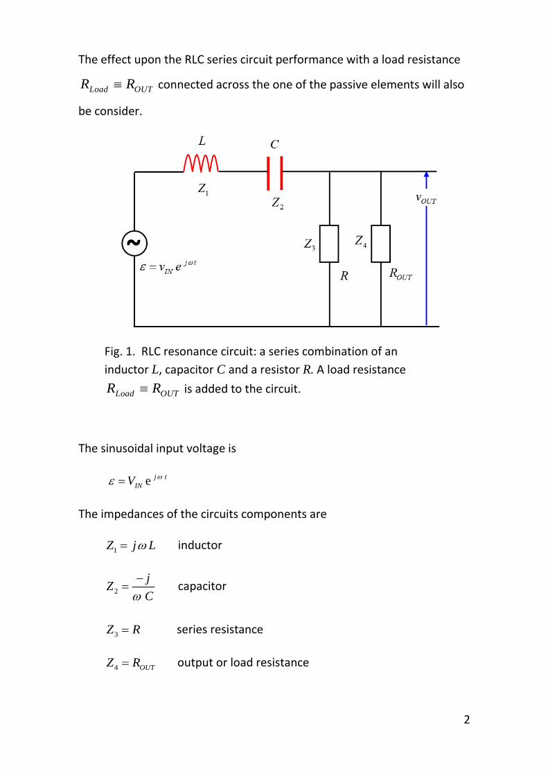
The effect upon the RLC series circuit performance with a load resistance
Load OUTR R connected across the one of the passive elements will also
be consider.
Fig. 1. RLC resonance circuit: a series combination of an
inductor L, capacitor C and a resistor R. A load resistance
Load OUTR R is added to the circuit.
The sinusoidal input voltage is
ej t
INV
The impedances of the circuits components are
1
Z j L inductor
2
jZ
C
capacitor
3
Z R series resistance
4 OUT
Z R output or load resistance
Page 3
3
We simplify the circuit by combining circuit elements that are in series and
parallel.
Parallel combination of series resistance and load resistance
5
3 4
1
1 1Z
Z Z
Series combination: total impedance
6 1 2 5
Z Z Z Z
The current through each component and the potential difference across
each component is computed from
V
I V I ZZ
in the following sequence of calculations (figure 2)
1 2 1
6
1 1 1 2 2 2
1 2 3 4
3 43 4
3 4
IN
OUT IN OUT
OUT
VI I I
Z
V I Z V I Z
V V V V V V V
V VI I I
Z Z
Page 4
4
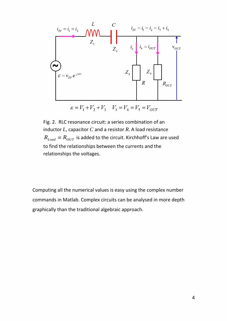
Fig. 2. RLC resonance circuit: a series combination of an
inductor L, capacitor C and a resistor R. A load resistance
Load OUTR R is added to the circuit. Kirchhoff’s Law are used
to find the relationships between the currents and the
relationships the voltages.
Computing all the numerical values is easy using the complex number
commands in Matlab. Complex circuits can be analysed in more depth
graphically than the traditional algebraic approach.
Page 5
5
The code below shows the main calculations that needed for the
simulations.
f = linspace(fMin,fMax, N); w = (2*pi).*f;
% impedances Z1 = 1i .* w .* L; % inductive impedance (reactance) Z2 = -1i ./ (w .*C); % capacitive impedance (reactance) Z3 = R; % series resistance Z4 = ROUT; % output or load resistance
Z5 = 1./ (1./Z3 + 1./Z4); % parallel combination Z6 = Z1 + Z2 + Z5; % total circuit impedance
% currents [A] and voltages [V] I1 = V_IN ./ Z6; I2 = I1; V1 = I1 .* Z1; V2 = I2 .* Z2; V_OUT = V_IN - V1 - V2; V3 = V_OUT; V4 = V_OUT; I3 = V_OUT ./ Z3; I4 = V_OUT ./ Z4;
% phases phi_OUT = angle(V_OUT); phi_1 = angle(V1); phi_2 = angle(V2);
theta_1 = angle(I1); theta_2 = angle(I2); theta_3 = angle(I3); theta_4 = angle(I4);
Page 6
6
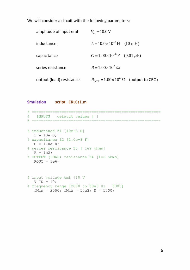
We will consider a circuit with the following parameters:
amplitude of input emf 10.0Vin
V
inductance 310.0 10 H (10 mH)L
capacitance 81.00 10 F (0.01 F)C
series resistance 21.00 10R
output (load) resistance 61.00 10
OUTR (output to CRO)
Smulation script CRLCs1.m
% ======================================================== % INPUTS default values [ ] % ========================================================
% inductance Z1 [10e-3 H] L = 10e-3; % capacitance Z2 [1.0e-8 F] C = 1.0e-8; % series resistance Z3 [ 1e2 ohms] R = 1e2; % OUTPUT (LOAD) resistance Z4 [1e6 ohms] ROUT = 1e6;
% input voltage emf [10 V] V_IN = 10; % frequency range [2000 to 50e3 Hz 5000] fMin = 2000; fMax = 50e3; N = 5000;
Page 7
7
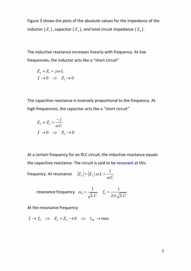
Figure 3 shows the plots of the absolute values for the impedance of the
inductor 1Z , capacitor 2
Z , and total circuit impedance 6Z .
The inductive reactance increases linearly with frequency. At low
frequencies, the inductor acts like a “short circuit”
1
10 0
LZ Z j L
f Z
The capacitive reactance is inversely proportional to the frequency. At
high frequencies, the capacitor acts like a “short circuit”
2
20 0
C
jZ Z
C
f Z
At a certain frequency for an RLC circuit, the inductive reactance equals
the capacitive reactance. The circuit is said to be resonant at this
frequency. At resonance L CZ Z
1L
C
resonance frequency 0 0
1 1
2f
LC LC
At the resonance frequency
00 max
L C INf f Z Z I
Page 8
8
Fig. 3. The magnitude of the impedances for the capacitor,
inductor and parallel combination as functions of frequency of
the source. A sharp peak occurs at the resonance frequency for
the impedance of the parallel combination.
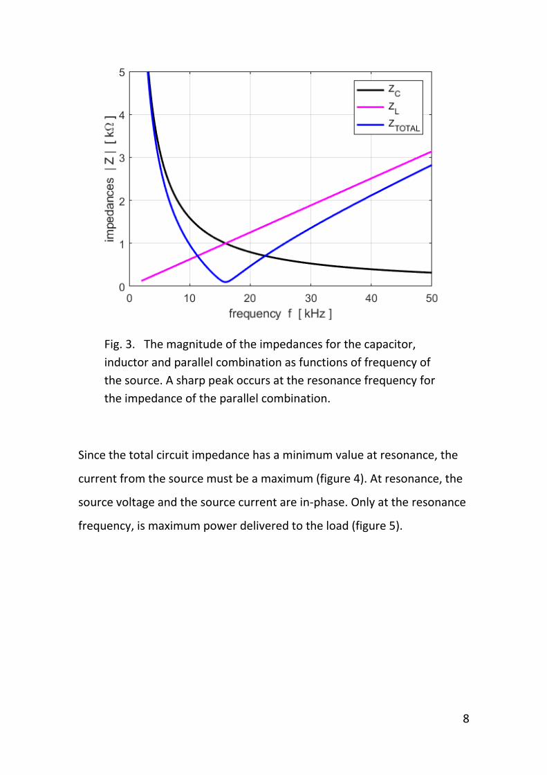
Since the total circuit impedance has a minimum value at resonance, the
current from the source must be a maximum (figure 4). At resonance, the
source voltage and the source current are in-phase. Only at the resonance
frequency, is maximum power delivered to the load (figure 5).
Page 9
9
Fig. 4. The source current has a maximum at the resonance
frequency. At resonance, the source voltage and source current
are in-phase with each other.
Fig. 5. Maximum power is delivered to the load at the
resonance frequency.
Page 10
10
The resonance frequency of the circuit is
0
1
2f
LC
The quality factor Q is a measure of the width of the current against
frequency plot. The power drops by half (-3 dB) at the half power
frequencies 1
f and 2
f where max/ 1 / 2
INI I . These two frequencies
determine the bandwidth f of the current.
2 1
f f f
It can be shown that the quality factor Q is
0f
Qf
The higher the Q value of a resonance circuit, the narrow the bandwidth
and hence the better the selectivity of the tuning.
The code for determination of the bandwidth:
% Resonance frequencies and Bandwidth calculations f0 = 1/(2*pi*sqrt(L*C)); Ipeak = max(abs(I1)); % max input current k = find(abs(I1) == Ipeak); % index for peak voltage gain f_peak = f(k); % frequency at peak I3dB = Ipeak/sqrt(2); % 3 dB points kB = find(abs(I1) > I3dB); % indices for 3dB peak k1 = min(kB); f1 = f(k1); k2 = max(kB); f2 = f(k2); df = f2-f1; % bandwidth Q = f0 / df; % quality factor
Page 11
11
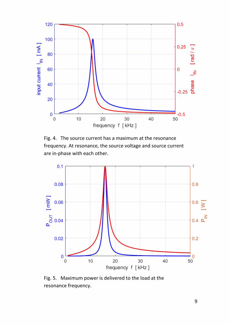
Figure 6 shows the current plot indicating the resonance frequency, half
power frequencies and the bandwidth.
Fig. 6. The current plot indicating the resonance frequency, half
power frequencies and the bandwidth.
A summary of the calculations is displayed in the Command Window
theoretical resonance frequency f0 = 15915 Hz
peak frequency f_peak = 15915 Hz
half power frequencies f1 = 15140 Hz 16730 Hz
bandwidth df = 1590 Hz
quality factor Q = 10.01
fprintf('theoretical resonance frequency f0 = %3.0f Hz
\n',f0);
fprintf('peak frequency f_peak = %3.0f Hz \n',f_peak);
fprintf('half power frequencies f1 = %3.0f Hz %3.0f Hz
\n',f1,f2);
fprintf('bandwidth df = %3.0f Hz \n',df);
fprintf('quality factor Q = %3.2f \n',Q);
Page 12
12
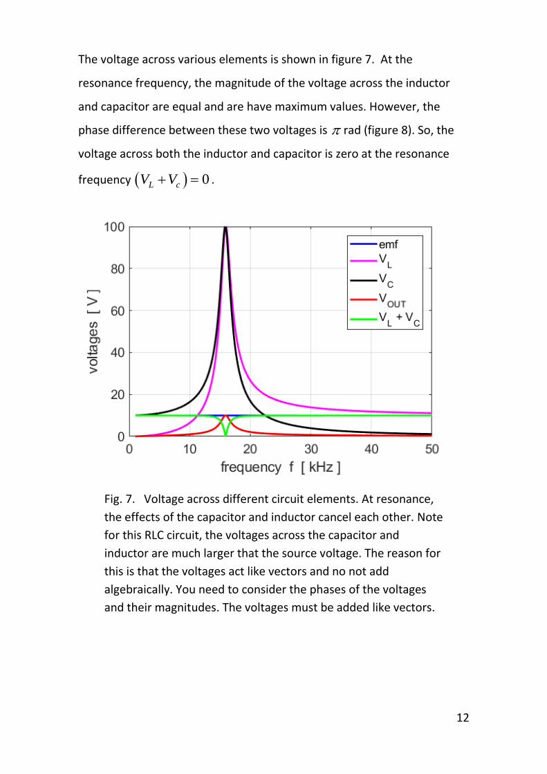
The voltage across various elements is shown in figure 7. At the
resonance frequency, the magnitude of the voltage across the inductor
and capacitor are equal and are have maximum values. However, the
phase difference between these two voltages is rad (figure 8). So, the
voltage across both the inductor and capacitor is zero at the resonance
frequency 0L cV V .
Fig. 7. Voltage across different circuit elements. At resonance,
the effects of the capacitor and inductor cancel each other. Note
for this RLC circuit, the voltages across the capacitor and
inductor are much larger that the source voltage. The reason for
this is that the voltages act like vectors and no not add
algebraically. You need to consider the phases of the voltages
and their magnitudes. The voltages must be added like vectors.
Page 13
13
Fig. 8. At resonance, / 2 rad / 2 radL C
and the
two voltages have the same magnitudes. Therefore, the effects
of the capacitance and inductance cancel each other, resulting
in a pure resistive impedance with the source voltage and
current in phase.
Kirchhoff’s Voltage Law states that the sum of the voltage drops around
the circuit is equal to the input emf to the circuit. For ac circuits, it is not
so straight forward to sum the voltages. You must account for the phases
of each current.
1 2 3V V V need to account for phase
abs(V1+V2+V3)
The emf is 10 V and at each frequency 1 2 3 10 VV V V .
Page 14
14
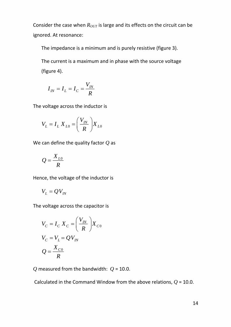
Consider the case when ROUT is large and its effects on the circuit can be
ignored. At resonance:
The impedance is a minimum and is purely resistive (figure 3).
The current is a maximum and in phase with the source voltage
(figure 4).
ININ L C
VI I I
R
The voltage across the inductor is
0 0IN
L L L L
VV I X X
R
We can define the quality factor Q as
0LXQ
R
Hence, the voltage of the inductor is
L INV QV
The voltage across the capacitor is
0
0
INC C C C
C L IN
C
VV I X X
R
V V QV
XQ
R
Q measured from the bandwidth: Q = 10.0.
Calculated in the Command Window from the above relations, Q = 10.0.
Page 15
15
We can also look at the behaviour of the circuit in the time domain and
gain a better understanding of how complex numbers give us information
about magnitudes and phases. The time domain equation for the currents
and voltages are
1
1
3
1
3
4
1 1
2 2
3 3
1 2 1
3 3
4 4
ej t
IN
j t
L
j t
C
j t
OUT R
j t
IN
j t
R
j t
RLoad
V
v v V e
v v V e
v v v V e
i i i I e
i i I e
i i I e
Each of the above relationships are plotted at a selected frequency which
is set within the script. The graphs below are for the resonance frequency
and the half-power frequencies.
c = 1; % c = 1 fs = f_peak; % c = 2 fs = f1; % c = 3 fs = f2 if c == 1; kk = k; fs = f_peak; kk = k; end if c == 2; kk = k1; fs = f1; end if c == 3; kk = k2; fs = f2; end Ns = 500; ws = 2*pi*fs; Ts = 1/fs; tMin = 0; tMax = 3*Ts; t = linspace(tMin,tMax,Ns); emf = real(V_IN .* exp(1j*ws*t)); v1 = real(abs(V1(kk)) .* exp(1j*(ws*t + phi_1(kk)))); v2 = real(abs(V2(kk)) .* exp(1j*(ws*t + phi_2(kk)))); v3 = real(abs(V3(kk)) .* exp(1j*(ws*t + phi_3(kk)))); i1 = real(abs(I1(kk)) .* exp(1j*(ws*t + theta_1(kk)))); i3 = real(abs(I3(kk)) .* exp(1j*(ws*t + theta_3(kk)))); i4 = real(abs(I4(kk)) .* exp(1j*(ws*t + theta_4(kk))));
Page 16
16
Fig. 9. The voltages at the resonance frequency and half-
power frequencies.
Page 17
17
Fig. 10. The currents at the resonance frequency and half-
power frequencies.
Page 18
18
Investigating the response of the RLC series circuit with
changes in parameters
You can simply change the input parameters and immediately
see the changes in the response of the circuit.
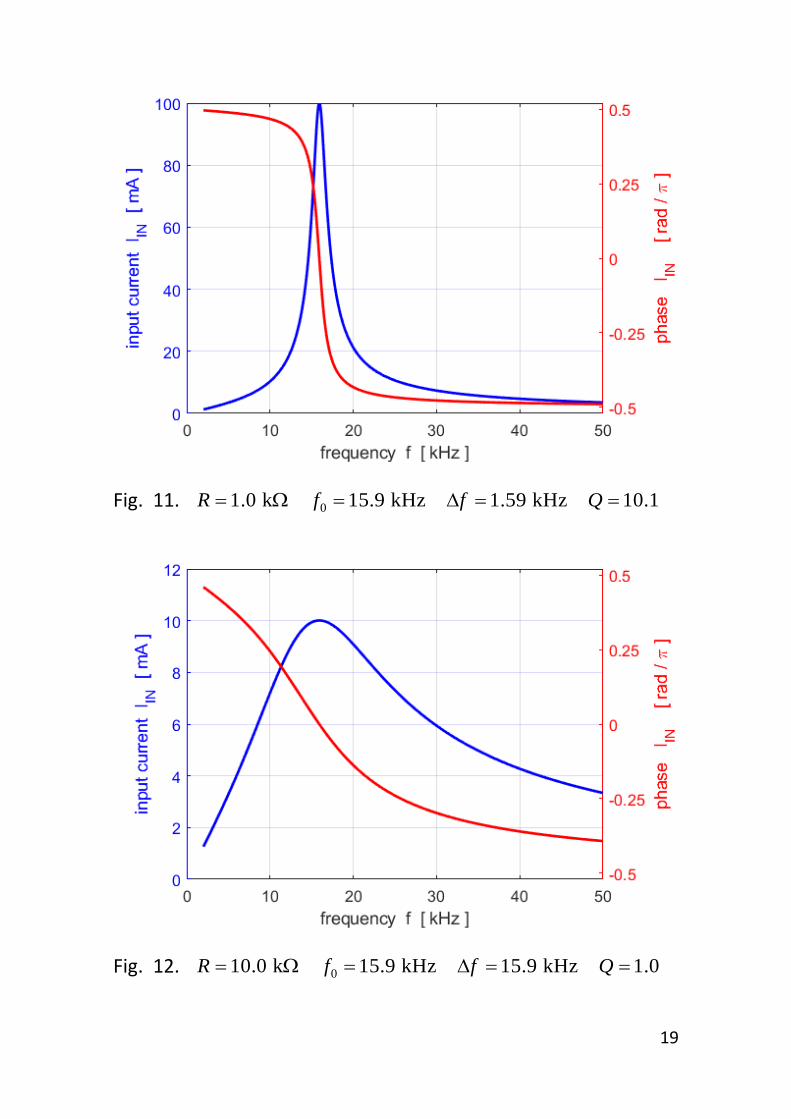
• Changing the value of the series resistance R does not
change the resonance frequency 0f . However, it does
change the sharpness of the current peak. As R is
increased, the bandwidth increases and the Q factor
decreases. Also, the current in the circuit decreases (figures
11 and 12).
Page 19
19
Fig. 11. 01.0 k 15.9 kHz 1.59 kHz 10.1R f f Q
Fig. 12. 010.0 k 15.9 kHz 15.9 kHz 1.0R f f Q
Page 20
20
• Decreasing the output resistance (load) ROUT slightly
decreases the bandwidth and increases the Q value, while
the current and power delivered to the load is increased
(figures 13 and 14).
Page 21
21
Fig. 13. 01.0 M 15.9 kHz 1.59 kHz 10.1OUTR f f Q
Fig. 14. 01.0 k 15.9 kHz 14.4 kHz 11.1OUTR f f Q
Page 22
22
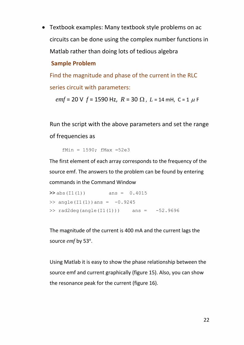
• Textbook examples: Many textbook style problems on ac
circuits can be done using the complex number functions in
Matlab rather than doing lots of tedious algebra
Sample Problem
Find the magnitude and phase of the current in the RLC
series circuit with parameters:
emf = 20 V f = 1590 Hz, R = 30 , L = 14 mH, C = 1 F
Run the script with the above parameters and set the range
of frequencies as
fMin = 1590; fMax =52e3
The first element of each array corresponds to the frequency of the
source emf. The answers to the problem can be found by entering
commands in the Command Window
>> abs(I1(1)) ans = 0.4015
>> angle(I1(1)) ans = -0.9245
>> rad2deg(angle(I1(1))) ans = -52.9696
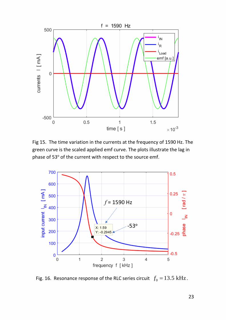
The magnitude of the current is 400 mA and the current lags the
source emf by 53o.
Using Matlab it is easy to show the phase relationship between the
source emf and current graphically (figure 15). Also, you can show
the resonance peak for the current (figure 16).
Page 23
23
Fig 15. The time variation in the currents at the frequency of 1590 Hz. The
green curve is the scaled applied emf curve. The plots illustrate the lag in
phase of 53o of the current with respect to the source emf.
Fig. 16. Resonance response of the RLC series circuit 0 13.5 kHzf .
Page 24
24
Modelling Experimental Data
Data was measured for the circuit shown in figure 1. An audio oscillator
was used for the source and the output was connected to digital storage
oscilloscope (DSO). The component values used were:
series resistance 31.00 10
SR
capacitance 81.0 10 F (0.01 F)C
inductance 3~ 5 10 HL
assume DSO resistance 61.00 10
OUTR (output to CRO)
The measurements are given in the script CRLCs2.m
Figure 11 shows a plot of the experimental data.
Fig. 11. Plot of the experimental measurements.
Page 25
25
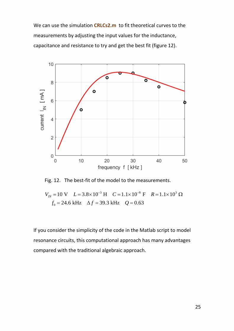
We can use the simulation CRLCs2.m to fit theoretical curves to the
measurements by adjusting the input values for the inductance,
capacitance and resistance to try and get the best fit (figure 12).
Fig. 12. The best-fit of the model to the measurements.
3 8 3
0
10 V 3.8 10 H 1.1 10 F 1.1 10
24.6 kHz 39.3 kHz 0.63
INV L C R
f f Q
If you consider the simplicity of the code in the Matlab script to model
resonance circuits, this computational approach has many advantages
compared with the traditional algebraic approach.
Page 26
26
DOING PHYSICS WITH MATLAB
http://www.physics.usyd.edu.au/teach_res/mp/mphome.htm
If you have any feedback, comments, suggestions or corrections
please email:
Ian Cooper School of Physics University of Sydney
[email protected]