173

Domain Adaptation with Coupled Subspaces

John Blitzer Dean Foster Sham KakadeGoogle Research University of Pennsylvania University of Pennsylvania

Abstract

Domain adaptation algorithms address a key is-sue in applied machine learning: How can wetrain a system under a source distribution butachieve high performance under a different tar-get distribution? We tackle this question for di-vergent distributions where crucial predictive tar-get features may not even have support under thesource distribution. In this setting, the key intu-ition is that that if we can link target-specific fea-tures to source features, we can learn effectivelyusing only source labeled data. We formalize thisintuition, as well as the assumptions under whichsuch coupled learning is possible. This allowsus to give finite sample target error bounds (us-ing only source training data) and an algorithmwhich performs at the state-of-the-art on two nat-ural language processing adaptation tasks whichare characterized by novel target features.

1 Introduction

The supervised learning paradigm of training and test-ing on identical distributions has provided a powerful ab-straction for developing and analyzing learning algorithms.In many natural applications, though, we train our algo-rithm on a source distribution, but we desire high per-formance on target distributions which differ from thatsource [20, 32, 6, 28]. This is the problem of domain adap-tation, which plays a central role in fields such as speechrecognition [25], computational biology [26], natural lan-guage processing [8, 11, 16], and web search [9, 15].1

In this paper, we address a domain adaptation setting that iscommon in the natural language processing literature. Our

1Jiang [22] provides a good overview of domain adaptationsettings and models

Appearing in Proceedings of the 14th International Conference onArtificial Intelligence and Statistics (AISTATS) 2011, Fort Laud-erdale, FL, USA. Volume 15 of JMLR: W&CP 15. Copyright2011 by the authors.

target domain contains crucial predictive features such aswords or phrases that do not have support under the sourcedistribution. Figure 1 shows two tasks which exemplify thiscondition. The left-hand side is a product review predictiontask [7, 12, 28]. The instances consist of reviews of differ-ent different products from Amazon.com, together with therating given to the product by the reviewer (1-5 stars). Theadaptation task is to build a regression model (for numberof stars) from reviews of one product type and apply it toanother. In the example shown, the target domain (kitchenappliances) contains phrases like a breeze which are posi-tive predictors but not present in the source domain.

The right-hand side of Figure 1 is an example of a part ofspeech (PoS) tagging task [31, 8, 19]. The instances consistof sequences of words, together with their tags (noun, verb,adjective, preposition etc). The adaptation task is to builda tagging model from annotated Wall Street Journal (WSJ)text and apply it to biomedical abstracts (BIO). In the ex-ample shown, BIO text contains words like opioid that arenot present in the WSJ.

While at first glance using unique target features withoutlabeled target data may may seem impossible, there is abody of empirical work achieving good performance in thissetting [8, 16, 19]. Such approaches are often referred toas unsupervised adaptation methods [17], and the intuitionthey have in common is that it is possible to use unla-beled target data to couple the weights for novel featuresto weights for features which are common across domains.For example, in the sentiment data set, the phrase a breezemay co-occur with the words excellent and good and thephrase highly recommended. Since these words are usedto express positive sentiment about books, we build a rep-resentation from unlabeled target data which couples theweight for a breeze with the weights for these features.

In contrast to the empirical work, previous theoreticalwork in unsupervised adaptation has focused on two set-tings. Either the source and target distributions share sup-port [18, 20, 10], or they have low divergence for a spe-cific hypothesis class [6, 28]. In the first setting, instanceweighting algorithms can achieve asymptotically target-optimal performance. In the second, it is possible to givefinite sample error bounds for specific hypothesis classes(although the models are not in general target-optimal).

174

John Blitzer, Dean Foster, Sham Kakade

Sentiment Classification Part of Speech Tagging

Books Financial News

Positive: packed with fascinating info NN VB VB NNNegative: plot is very predictable funds are attracting investors

Kitchen Appliances Biomedical Abstracts

Positive: a breeze to clean up NN PP ADJ NNNegative: leaking on my countertop expression of opioid receptors

Figure 1: Examples from two natural language processing adaptation tasks, where the target distributions contain words(in red) that do not have support under the source distribution. Words colored in blue and red are unique to the sourceand target domains, respectively. Sentiment classification is a binary (positive vs. negative) classification problem. Part ofspeech tagging is a sequence labeling task, where NN indicates noun, PP indicates preposition, VB indicates verb, etc.

Neither setting addresses the use of target-specific features,though, and instance weighting is known to perform poorlyin situations where target-specific features are important forgood performance [21, 22].

The primary contribution of this work is to formalize as-sumptions that: 1) allow for transferring an accurate classi-fier from our source domain to an accurate classifier on thetarget domain and 2) are capable of using novel featuresfrom the target domain. Based on these assumptions, wegive a simple algorithm that builds a coupled linear sub-space from unlabeled (source and target) data, as well asa more direct justification for previous “shared representa-tion” empirical domain adaptation work [8, 16, 19]. Wealso give finite source sample target error bounds that de-pend on how the covariance structure of the coupled sub-space relates to novel features in the target distribution.

We demonstrate the performance of our algorithm on thesentiment classification and part of speech tagging tasks il-lustrated in Figure 1. Our algorithm gives consistent perfor-mance improvements from learning a model on source la-beled data and testing on a different target distribution. Fur-thermore, incorporating small amounts of target data (alsocalled semi-supervised adaptation) is straightforward underour model, since our representation automatically incorpo-rates target data along those directions of the shared sub-space where it is needed most. In both of these cases, weperform comparable to state-of-the-art algorithms whichalso exploit target-specific features.

2 Setting

Our input X ∈ X are vectors, where X is a vector space.Our output Y ∈ R. Each domain D = d defines a jointdistribution Pr[X,Y |D = d] (where the domains are eithersource D = s or target D = t). Our first assumption is astronger version of the covariate shift assumption [18, 20,

10]. That is, there exists a single good linear predictor forboth domains:

Assumption 1. (Identical Tasks) Assume there there is avector β so that for d ∈ s, t:

E[Y |X,D = d] = β ·X

This assumption may seem overly strong, and for low-dimensional spaces it often is. As we show in section 5.5,though, for our tasks it holds, at least approximately.

Now suppose we have a labeled training data T = {(x, y)}on the source domain s, and we desire to perform well onour target domain t. Let us examine what is transferred byusing the naive algorithm of simply minimizing the squareloss on the source domain.

Roughly speaking, using samples from the source domains, we can estimate β in only those directions in which Xvaries on domain s. To make this precise, define the princi-pal subspaceXd for a domain d as the (lowest dimensional)subspace of X such that X ∈ Xd with probability 1.

There are three natural subspaces between the source do-main s and target domain t; the part which is shared andthe parts specific to each. More precisely, define the sharedsubspace for two domains s and t asXs,t = Xs∩Xt (the in-tersection of the principal subspaces, which is itself a sub-space). We can decompose any vector x into the vectorx = [x]s,t + [x]s,⊥ + [x]t,⊥, where the latter two vec-tors are the projections of x which lie off the shared sub-space (Our use of the “⊥” notation is justified since one canchoose an inner product space where these components areorthogonal, though our analysis does not explicitly assumeany inner product space on X ). We can view the naivealgorithm as fitting three components, [w]s,t, [w]s,⊥, and[w]t,⊥, where the prediction is of the form:

[w]s,t · [x]s,t + [w]s,⊥ · [x]s,⊥ + [w]t,⊥ · [x]t,⊥

175

John Blitzer, Dean Foster, Sham Kakade

Here, with only source data, this would result in an unspec-ified estimate of [w]t,⊥ as [x]t,⊥ = 0 for x ∈ Xs. Fur-thermore, the naive algorithm would only learn weights on[x]s,t (and it is this weight, on what is shared, which is whattransfers to the target domain).

Certainly, without further assumptions, we would not ex-pect to be able to learn how to utilize [x]t,⊥ with only train-ing data from the source. However, as discussed in theintroduction, we might hope that with unlabeled data, wewould be able to “couple” the learning of features in [x]t,⊥to those on [x]s,t.

2.1 Unsupervised Learning and DimensionalityReduction

Our second assumption specifies a means by which thiscoupling may occur. Given a domain d, there are a numberof semi-supervised methods which seek to find a projec-tion to a subspace Xd, which loses little predictive infor-mation about the target. In fact, much of the focus on un-(and semi-)supervised dimensionality reduction is on find-ing projections of the input space which lose little predic-tive power about the target. We idealize this with the fol-lowing assumption.

Assumption 2. (Dimensionality Reduction) For d ∈{s, t}, assume there is a projection operator 2 Πd and avector βd such that

E[Y |X,D = d] = βd · (ΠdX) .

Furthermore, as Πt need only be specified on Xt for thisassumption, we can specify the target projection operatorso that Πt[x]s,⊥ = 0 (for convenience).

Implicitly, we assume that Πs and Πt can be learned fromunlabeled data, and being able to do so is is crucial to thepractical success of an adaptation algorithm in this setting.Practically, we already know this is possible from empiricaladaptation work [8, 16, 19].

3 Adaptation Algorithm

Under Assumptions 1 and 2 and given labeled source dataand unlabeled source and target data, the high-level viewof our algorithm is as follows: First, estimate Πs and Πt

from unlabeled source and target data. Then, use Πs andΠt to learn a target predictor from source data. We beginby giving one algorithm for estimating Πs and Πt, but weemphasize that any Πs and Πt which satisfy Assumption 2are appropriate under our theory. Our focus here is to showhow we can exploit these projections to achieve good tar-get results, and in Section 5.1 we analyze and evaluate thestructural correspondence learning [8] method, as well.

2Recall, that M is a projection operator if M is a linear and ifM is idempotent, i.e. M2x = Mx

Input: Unlabeled source and target dataxs, xt.

Output: Πs, Πt

1. For source and target domains d,a. ∀xd, Divide xd into multiple

views x(1)d and x

(2)d .

b. Choose k < min(D1, D2) features

from each view(x(1)d,ij

)kj=1

.

c. Construct the D1 × k and D2 × k

cross-correlation matrices C12 & C21,

where C12ij =

x(1)d,i

x(2)d,ij√

x(1)d,i

x(1)d,i

x(2)d,ij

x(2)d,ij

.

d. Let Πd =

[Π

(1)d 0

0 Π(2)d

], where Π

(1)d is

the outer product of the top leftsingular vectors of C12 (likewise

with Π(2)d and C21.

2. Return Πs and Πt.

Figure 2: Algorithm for learning Πs and Πt.

3.1 Estimating Πs, Πt and [x]s,⊥

Figure 2 describes the algorithm we use for learning Πs

and Πt. It is modeled after the approximate canonical cor-relation analysis algorithm of Ando et al. [2, 23, 14], whichalso forms the basis of the SCL domain adaptation algo-rithm [8]. CCA is a multiple-view dimensionality reduc-tion algorithm, so we begin by breaking up each instanceinto two views (1a). For the sentiment task, we split thefeature space up randomly, with half of the features in oneview and half in the other. For the PoS task, we build rep-resentations for each word in the sequence by dividing upfeatures into those that describe the current word and thosethat describe its context (the surrounding words).

After defining multiple views, we build the the cross-correlation matrix between views. For our tasks, where fea-tures describe words or bigrams, each view can be hundredsof thousands of dimensions. The cross-correlation matri-ces are dense and too large to fit in memory, so we adoptan approximation technique from Ando et al. [2, 14]. Thisrequires choosing k representative features and building alow-rank cross-correlation matrix from these (1b). Nor-mally, we would normalize by whitening using the within-view covariance matrix. Instead of this, we use simple cor-relations, which are much faster to compute (requiring onlya single pass over the data) and worked just as well in ourexperiments (1c). The singular value decomposition of thecross-correlation matrix yields the top canonical correla-tion directions, which we combine to form Πs and Πt (1d).

176

John Blitzer, Dean Foster, Sham Kakade

fasc

inat

ing

shared

(a)

fasc

inat

ing

(b)

fasc

inat

ing

(c)

fasc

inat

ing

(d)

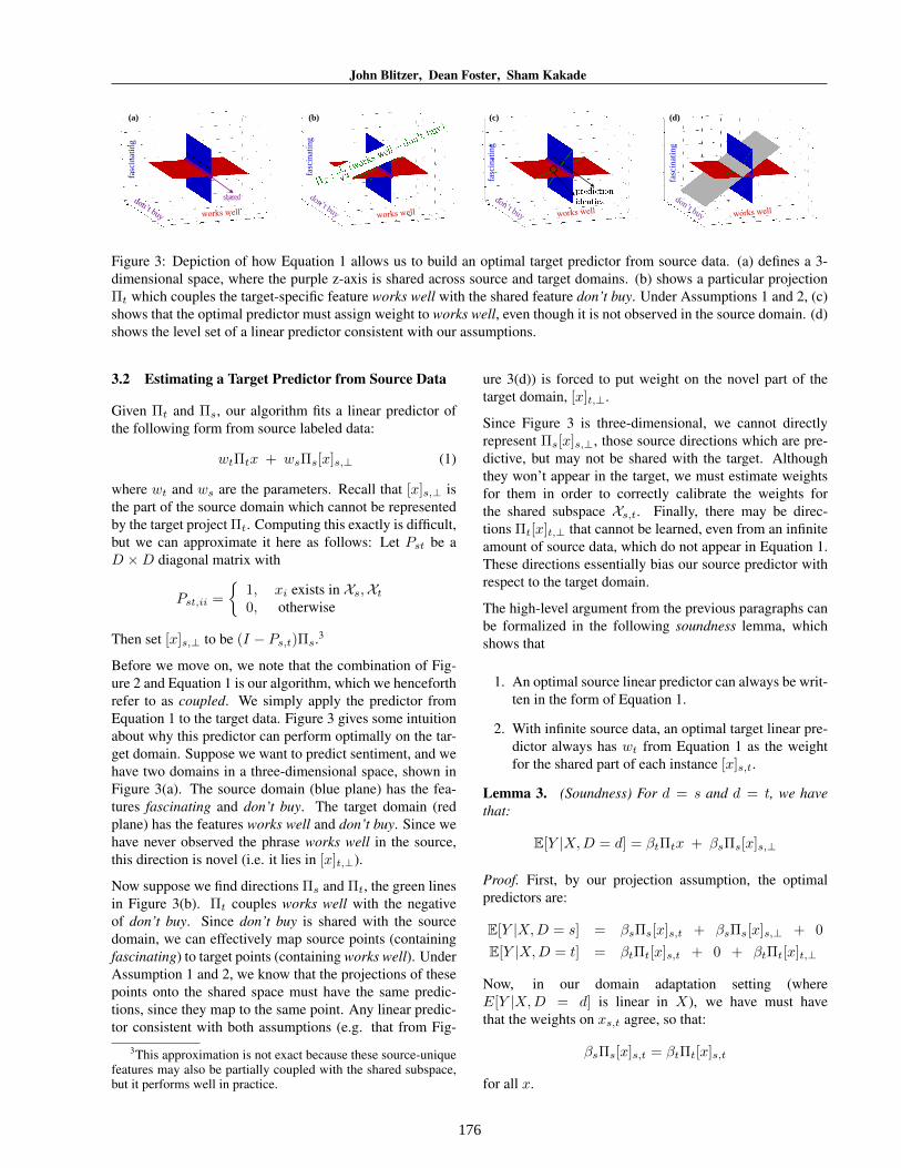
Figure 3: Depiction of how Equation 1 allows us to build an optimal target predictor from source data. (a) defines a 3-dimensional space, where the purple z-axis is shared across source and target domains. (b) shows a particular projectionΠt which couples the target-specific feature works well with the shared feature don’t buy. Under Assumptions 1 and 2, (c)shows that the optimal predictor must assign weight to works well, even though it is not observed in the source domain. (d)shows the level set of a linear predictor consistent with our assumptions.

3.2 Estimating a Target Predictor from Source Data

Given Πt and Πs, our algorithm fits a linear predictor ofthe following form from source labeled data:

wtΠtx + wsΠs[x]s,⊥ (1)

where wt and ws are the parameters. Recall that [x]s,⊥ isthe part of the source domain which cannot be representedby the target project Πt. Computing this exactly is difficult,but we can approximate it here as follows: Let Pst be aD ×D diagonal matrix with

Pst,ii =

{1, xi exists in Xs,Xt0, otherwise

Then set [x]s,⊥ to be (I − Ps,t)Πs.3

Before we move on, we note that the combination of Fig-ure 2 and Equation 1 is our algorithm, which we henceforthrefer to as coupled. We simply apply the predictor fromEquation 1 to the target data. Figure 3 gives some intuitionabout why this predictor can perform optimally on the tar-get domain. Suppose we want to predict sentiment, and wehave two domains in a three-dimensional space, shown inFigure 3(a). The source domain (blue plane) has the fea-tures fascinating and don’t buy. The target domain (redplane) has the features works well and don’t buy. Since wehave never observed the phrase works well in the source,this direction is novel (i.e. it lies in [x]t,⊥).

Now suppose we find directions Πs and Πt, the green linesin Figure 3(b). Πt couples works well with the negativeof don’t buy. Since don’t buy is shared with the sourcedomain, we can effectively map source points (containingfascinating) to target points (containing works well). UnderAssumption 1 and 2, we know that the projections of thesepoints onto the shared space must have the same predic-tions, since they map to the same point. Any linear predic-tor consistent with both assumptions (e.g. that from Fig-

3This approximation is not exact because these source-uniquefeatures may also be partially coupled with the shared subspace,but it performs well in practice.

ure 3(d)) is forced to put weight on the novel part of thetarget domain, [x]t,⊥.

Since Figure 3 is three-dimensional, we cannot directlyrepresent Πs[x]s,⊥, those source directions which are pre-dictive, but may not be shared with the target. Althoughthey won’t appear in the target, we must estimate weightsfor them in order to correctly calibrate the weights forthe shared subspace Xs,t. Finally, there may be direc-tions Πt[x]t,⊥ that cannot be learned, even from an infiniteamount of source data, which do not appear in Equation 1.These directions essentially bias our source predictor withrespect to the target domain.

The high-level argument from the previous paragraphs canbe formalized in the following soundness lemma, whichshows that

1. An optimal source linear predictor can always be writ-ten in the form of Equation 1.

2. With infinite source data, an optimal target linear pre-dictor always has wt from Equation 1 as the weightfor the shared part of each instance [x]s,t.

Lemma 3. (Soundness) For d = s and d = t, we havethat:

E[Y |X,D = d] = βtΠtx + βsΠs[x]s,⊥

Proof. First, by our projection assumption, the optimalpredictors are:

E[Y |X,D = s] = βsΠs[x]s,t + βsΠs[x]s,⊥ + 0

E[Y |X,D = t] = βtΠt[x]s,t + 0 + βtΠt[x]t,⊥

Now, in our domain adaptation setting (whereE[Y |X,D = d] is linear in X), we have must havethat the weights on xs,t agree, so that:

βsΠs[x]s,t = βtΠt[x]s,t

for all x.

177

John Blitzer, Dean Foster, Sham Kakade

For d = t, the above holds since [x]s,⊥ = 0 for x ∈ Xt.For d = s, we have Πtx = Πt[x]s,t + Πt[x]s,⊥ = Πt[x]s,tfor x ∈ Xs, since Πt is null on [x]s,⊥ (as discussed inAssumption 2).

In the next section, we will prove two important conse-quences of Lemma 3, demonstrating when we can learn aperfect target predictor from only source training data andat what rate (in terms of source data) this predictor willconverge.

4 Learning Bounds for the CoupledRepresentation

We begin by stating when we converge to a perfect targetpredictor on the target domain with a sufficiently large la-beled source sample.

Theorem 4. (Perfect Transfer) Suppose ΠtXs,t = ΠtXt.Then any weight vector (wt, ws) on the coupled represen-tation which is optimal on the source, is also optimal on thetarget.

Proof. If (wt, ws) provides an optimal prediction on s,then this uniquely (and correctly) specifies the linear mapon Xs,t. Hence, wt is such that wtΠt[x]s,t is correct forall x, e.g. wtΠt[x]s,t = β[x]s,t (where β is as definedin Assumption 1). This implies that wt has been correctlyspecified in dim(ΠtXs,t) directions. By assumption, thisimplies that all directions for wt have been specified, asΠtXs,t = ΠtXt

Our next theorem describes the ability of our algorithm togeneralize from finite training data (which could consist ofonly source samples or a mix of samples from the sourceand target). For the theorem, we condition on the inputs xin our training set (e.g. we work in a fixed design setting).In the fixed design setting, the randomization is only overthe Y values for these fixed inputs. Define the followingtwo covariance matrices:

Σt = E[ (Πtx)(Πtx)>|D = t],

Σs→t =1

n

∑x∈Ts

(Πtx)(Πtx)>

Roughly speaking, Σs→t specifies how the training inputsvary in the relevant target directions.

Theorem 5. (Generalization) Assume that Var(Y |X) ≤1. Let: our coordinate system be such that Σt = I; Lt(w)be the square loss on the target domain; and (wt, ws) bethe empirical risk minimizer with a training sample of sizen. Then our expected regret is:

E[Lt(wt, ws)]− Lt(βt, βs) ≤∑i

1λi

n

where λi are the eigenvalues of Σs→t and the expectationis with respect to random samples of Y on the fixed traininginputs.

The proof is in Appendix A. For the above bound to bemeaningful we need the eigenvalues λi to be nonzero – thisamounts to having variance in all the directions in ΠtXt (asthis is the subspace corresponding to target error covari-ance matrix Σt). It is possible to include a bias term for ourbound (as a function of βt) in the case when some λi = 0,though due to space constraints, this is not provided. Fi-nally, we note that incorporating target data is straightfor-ward under this model. When Σt = I , adding target datawill (often significantly) reduce the inverse eigenvalues ofΣs→t, providing for better generalization. We demonstratein Section 5 how simply combining source and target la-beled data can provide improved results in our model.

We briefly compare our bound to the adaptation generaliza-tion results of Ben-David et al. [4] and Mansour et al. [27].These bounds factor as an approximation term that goes to0 as the amount of source data goes to infinity and a biasterm that depends on the divergence between the two dis-tributions. If perfect transfer (Theorem 4) is possible, thenour bound will converge to 0 without bias. Note that The-orem 4 can hold even when there is large divergence be-tween the source and target domains, as measured by Ben-David et al. [4] and Mansour et al. [27]. On the other hand,there may be situations where for finite source samples ourbound is much larger due to small eigenvalues of Σs→t.

5 Experiments

We evaluate our coupled learning algorithm (Equation 1)together with several other domain adaptation algorithmson the sentiment classification and part of speech taggingtasks illustrated in Figure 1. The sentiment predictiontask [7, 28, 12] consists of reviews of four different typesof products: books, DVDs, electronics, and kitchen appli-ances from Amazon.com. Each review is associated witha rating (1-5 stars), which we will try to predict. Thesmallest product type (kitchen appliances) contains approx-imately 6,000 reviews. The original feature space of un-igrams and bigrams is on average approximately 100,000dimensional. We treat sentiment prediction as a regressionproblem, where the goal is to predict the number of stars,and we measure square loss.

The part-of-speech tagging data set [8, 19, 30] is a muchlarger data set. The two domains are articles from the WallStreet Journal (WSJ) and biomedical abstracts from MED-LINE (BIO). The task is to annotate words with one of 39tags. For each domain, we have approximately 2.5 mil-lion words of raw text (which we use to learn Πs and Πt),but the labeling conditions are quite asymmetric. The WSJcorpus contains the Penn Treebank corpus of 1 million an-

178

John Blitzer, Dean Foster, Sham Kakade

notated words [29]. The BIO corpus contains only approx-imately 25 thousand annotated words, however.

We model sentences using a first-order conditional randomfield (CRF) tagger [24]. For each word, we extract fea-tures from the word itself and its immediate one-word leftand right context. As an example context, in Figure 1, thewindow around the word opioid is of on the left and re-ceptors on the right. The original feature space consistsof these words, along with character prefixes and suffixesand is approximately 200,000 dimensional. Combined with392 tags, this gives approximately 300 million parametersto estimate in the original feature space. The CRF does notminimize square loss, so Theorem 5 cannot be used directlyto bound its error. Nonetheless, we can still run the coupledalgorithm from Equation 1 and measure its error.

There are two hyper-parameters of the algorithm from Fig-ure 2. These are the number of features k we choose whenwe compute the cross-correlation matrix and the dimen-sionality of Πs and Πt. k is set to 1000 for both tasks.For sentiment classification, we chose a 100-dimensionalrepresentation. For part of speech tagging, we chose a 200-dimensional representation for each word (left, middle, andright). We use these throughout all of our experiments,but in preliminary investigation the results of our algorithmwere fairly stable (similar to those of Ando and Zhang [1])across different settings of this dimensionality .

5.1 Adaptation Models

Here we briefly describe the models we evaluated in thiswork. Not all of them appear in the subsequent figures.

Naıve. The most straightforward model ignores the targetdata and trains a model on the source data alone.

Ignore source-specific features. If we believed that thegap in target domain performance was primarily due tosource-specific features, rather than target-specific fea-tures, we might consider simply discarding those featuresin the source domain which don’t appear in the target. Ourtheory indicates that these can still be helpful (Lemma 3 nolonger holds without them), and discarding these featuresnever helped in any experiment. Because of this, we do notreport any numbers for this model.

Instance Weighting. Instance weighting approaches toadaptation [20, 5] are asymptotically optimal and canperform extremely well when we have low-dimensionalspaces. They are not designed for the case when new targetdomain features appear, though. Indeed, sample selectionbias correction theory [20, 28] does not yield meaningfulresults when distributions do not share support. We ap-plied the instance weighting method of Bickel [5] to thesentiment data and did not observe consistent improvementover the naıve baseline. For the part of speech tagging,we did not apply instance weighting, but we note the work

of Jiang [21], who experimented with instance weightingschemes for this task and saw no improvement over a naıvebaseline. We do not report instance weighting results here.

Use Πt. One approach to domain adaptation is to treatit as a semi-supervised learning problem. To do this, wesimply estimate a prediction wtΠtx for x ∈ Xs, ignoringsource-specific features. According to Equation 1, this willperform worse than accounting for [x]s,⊥, but it can stillcapture important target-specific information. We note thatthis is essentially the semi-supervised algorithm of Ando etal. [2], treating the target data as unlabeled.

Coupled. This method estimates Πs, Πt, and [x]s,⊥ usingthe algorithm in Figure 2. Then it builds a target predictorfollowing Equation 1 and uses this for target prediction.

Correspondence. This is our re-implementation of thestructural correspondence learning (SCL) algorithm of [8].This algorithm learns a projection similar to the one fromFigure 2, but with two differences. First, it concatenatessource and target data and learns a single projection Π. Sec-ond, it only uses, as its k representative features from eachview, features which are shared across domains.

One way to view SCL under our theory is to divide Π intoΠs and Πt by copying it and discarding the target-specificfeatures from the first copy and the source-specific featuresfrom the second copy. With this in hand, the rest of SCL isjust following Equation 1. At a high level, correspondencecan perform better than coupled when the shared space islarge and coupled ignores some of it. Coupled can performbetter when the shared space is small, in which case it mod-els domain-specific spaces [x]s,⊥, [x]t,⊥ more accurately.

5.2 Adaptation with Source Only

We begin by evaluating the target performance of our cou-pled learning algorithm when learning only from labeledsource data. Figure 4 shows that all of the algorithms whichlearn some representation for new target features never per-form worse than the naıve baseline. Coupled never per-forms worse than the semi-supervised Πt approach, andcorrespondence performs worse only in one pair (DVDs toelectronics). It is also worth mentioning that certain pairsof domains overlap more than others. Book and DVD re-views tend to share vocabulary. So do kitchen applianceand electronics reviews. Across these two groups (e.g.books versus kitchen appliances), reviews do not share alarge amount of vocabulary. For the eight pairs of domainswhich do not share significant vocabulary, the error bars ofcoupled and the naıve baseline do not overlap, indicatingthat coupled consistently outperforms the baseline.

Figure 5 illustrates the coupled learner for part of speechtagging. In this case, the variance among experiments ismuch smaller due to the larger training data. Once again,coupled always improves over the naıve model. Because

179

John Blitzer, Dean Foster, Sham Kakade

DVD Electr Kitch

1.31.51.71.9

Boo

ksBooks Electr Kitch

1.41.55

1.71.85

DV

D

Naive

ΠT

Couple

Corres.

Target

Books DVD Kitch

1.21.41.61.8

Ele

ctro

n

Books DVD Electr

1.151.31.51.7

Kitc

hen

Figure 4: Squared error for the sentiment data (1-5 stars). Each of the four graphs shows results for a single target domain,which is labeled on the Y-axis. Clockwise from top left are books, dvds, kitchen, and electronics. Each group of fivebars represents one pair of domains, and the error bars indicate the standard deviation over 10 random draws of sourcetraining and target test set. The red bar is the naıve algorithm which does not exploit Πt or Πs. The green uses Πtx but notΠs[x]s,⊥. The purple is the coupled learning algorithm from Equation 1. The yellow is our re-implementation of SCL [8],and the blue uses labeled target training data, serving as a ceiling on improvement.

WSJ

4

6

8

10

12

14

Trg

: BIO

BIO

6

12

18

24

30

Trg

: WSJ

NaiveCoupledCorresTargetSCL*

Figure 5: Per-token error for the part of speech taggingtask. Left is from WSJ to BIO. Right is from BIO to WSJ.The algorithms are the same as in Figure 4.

of data asymmetry, the WSJ models perform much bet-ter on BIO than vice versa. Finally, we also report, forthe WSJ→BIO task, the SCL error reported by Blitzer etal. [8]. This error rate is much lower than ours, and webelieve this to be due to differences in the features used.They used a 5-word (rather than 3-word) window, includedbigrams of suffixes, and performed separate dimensional-ity reductions for each of 25 feature types. It would al-most certainly be helpful to incorporate similar extensionsto coupled, but that is beyond the scope of this work.

5.3 Adaptation with Source and Target

Our theory indicates that target data can be helpful in sta-bilizing predictors learned from the source domain, espe-cially when the domains diverge somewhat on the sharedsubspace. Here we show that our coupled predictors con-tinue to consistently improve over the naıve predictors,even when we do have labeled target training data. Figure 6

demonstrates this for three selected domain pairs. In thecase of part of speech tagging, we use all of the availabletarget labeled data, and in this case we see an improvementover the target only model. Since the relative relationshipbetween coupled and correspond remain constant, we donot depict that here. We also do not show results for allpairs of domains, but these are representative.

Finally, we note that while Blitzer et al. [8, 7] successfullyused labeled target data for both of these tasks, they usedtwo different, specialized heuristics for each. In our set-ting, combining source and target data is immediate fromTheorem 5, and simply applying the coupled predictor out-performs the baseline for both tasks.

5.4 Use of target-specific features

Here we briefly explore how the coupled learner putsweight on unseen features. One simple test is to measurethe relative mass of the weight vector that is devoted totarget-specific features under different models. Under thenaıve model, this is 0. Under the shared representation, itis the proportion of wtΠt devoted to genuinely unique fea-

tures. That is,||[wtΠt]t,⊥||

22

||wtΠt||22. This quantity is on average

9.5% across all sentiment adaptation task pairs and 32%for part of speech tag adaptation. A more qualitative wayto observe the use of target specific features is shown infigure 5.4. Here we selected the top target-specific words(never observed in the source) that received high weightunder wtΠt. Intuitively, the ability to assign high weightto words like illustrations when training on only kitchenappliances can help us generalize better.

180

John Blitzer, Dean Foster, Sham Kakade

0 50 100 200 5001.11.21.31.41.51.61.7

Books → Kitch

Kitchen0 50 100 200 500

1.31.41.51.61.71.81.9

Elec → DVD

DVD0 50 100 200 500

45.5

78.510

11.513

WSJ → BIO

BIO

Naive

Coupled

Target

Figure 6: Including target labeled data. Each figure represents one pair of domains. The x axis is the amount of target data.

Adaptation Negative Target Features Positive Target FeaturesBooks to Kitch mush, bad quality, broke, warranty, coffeemaker dishwasher, evenly, super easy, works great, great productKitch to Books critique, trite, religious, the publisher, the author introduction, illustrations, good reference, relationships

Figure 7: Illustration of how the coupled learner (Equation 1) uses unique target-specific features for the pair of sentimentdomains Books and Kitchen. We train a model using only source data and then find the most positive and negative featuresthat are target specific by examining the weights under [wtΠt]t,⊥.

5.5 Validity of Assumptions

Our theory depends on Assumptions 1 and 2, but we do notexpect these assumptions to hold exactly in practice. Bothassumptions state a linear mean for (Y |X), and we notethat for standard linear regression, much analysis is doneunder the linear mean assumption, even though it is difficultto test if it holds. In our case, the spirit of our assumptionscan be tested independently of the linear mean assumption:Assumption 1 is an idealization of the existence of a singlegood predictor for both domains, and Assumption 2 is anidealization of the existence of projection operators whichdo not degrade predictor performance. We show here thatboth assumptions are reasonable for our domains.

Assumption 1. We empirically test that there there is onesimultaneously good predictor on each domain. To see thatthis is approximately true, we train by mixing both do-mains, w∗= argminw [Ls(w) + Lt(w)], and compare thatwith a model trained on a single domain. For the domainpair books and kitchen appliances, training a joint predic-tor on books and kitchen appliance reviews together resultsin a 1.38 mean squared error on books, versus 1.35 if wetrain a predictor from books alone. Other sentiment domainpairs are similar. For part-of-speech tagging, measuring er-ror on the Wall Street Journal, we found 4.2% joint errorversus 3.7% WSJ-only error. These relatively minor per-formance differences indicate that one good predictor doesexist for both domains.

Assumption 2. We test that the projection operator causeslittle degradation as opposed to using a complete represen-tation. Using the projection operator, we train as usual, andwe compare that with a model trained on the original, high-

dimensional feature space. With large amounts of trainingdata, we know that the original feature space is at least asgood as the projected feature space. For the electronicsdomain, the reduced-dimensional representation achieves a1.23 mean squared error versus a 1.21 for the full repre-sentation. Other sentiment domain pairs are similar. Forthe Wall Street Journal, the reduced dimensional represen-tation achieves 4.8% error versus 3.7% with the original.These differences indicate that we found a good projectionoperator for sentiment, and a projections operator with mi-nor violations for part of speech tagging.

6 Conclusion

Domain adaptation algorithms have been extensively stud-ied in nearly every field of applied machine learning. Whatwe formalized here, for the first time, is how to adapt fromsource to target when crucial target features do not havesupport under the source distribution. Our formalizationleads us to suggest a simple algorithm for adaptation basedon a low-dimensional coupled subspace. Under natural as-sumptions, this algorithm allows us to learn a target predic-tor from labeled source and unlabeled target data.

One area of domain adaptation which is beyond the scopeof this work, but which seen much progress recently, is su-pervised and semi-supervised adaptation [3, 13, 17]. Thiswork focuses explicitly on using labeled data to relax oursingle-task Assumption 1. Since these methods also makeuse of shared subspaces, it is natural to consider combina-tions of them with our coupled subspace approach, and welook forward to exploring these possibilities further.

181

John Blitzer, Dean Foster, Sham Kakade

References[1] R. Ando and T. Zhang. A framework for learning pre-

dictive structures from multiple tasks and unlabeleddata. JMLR, 6:1817–1853, 2005.

[2] R. Ando and T. Zhang. Two-view feature generationmodel for semi-supervised learning. In ICML, 2007.

[3] A. Arygriou, C. Micchelli, M. Pontil, and Y. Yang.A spectral regularization framework for multi-taskstructure learning. In NIPS, 2007.

[4] S. Ben-David, J. Blitzer, K. Crammer, and F. Pereira.Analysis of representations for domain adaptation. InNIPS, 2007.

[5] S. Bickel, M. Bruckner, and T. Scheffer. Discrimi-native learning for differing training and test distribu-tions. In ICML, 2007.

[6] J. Blitzer, K. Crammer, A. Kulesza, and F. Pereira.Learning bounds for domain adaptation. In NIPS,2008.

[7] J. Blitzer, M. Dredze, and F. Pereira. Biographies,bollywood, boomboxes and blenders: Domain adap-tation for sentiment classification. In ACL, 2007.

[8] J. Blitzer, R. McDonald, and F. Pereira. Domain adap-tation with structural correspondence learning. InEMNLP, 2006.

[9] K. Chen, R. Liu, C.K. Wong, G. Sun, L. Heck, andB. Tseng. Trada: tree based ranking function adapta-tion. In CIKM, 2008.

[10] C. Cortes, M. Mohri, M. Riley, and A. Rostamizadeh.Sample selection bias correction theory. In ALT,2008.

[11] Hal Daume, III. Frustratingly easy domain adapta-tion. In ACL, 2007.

[12] M. Dredze and K. Crammer. Online methods formulti-domain learning and adaptation. In EMNLP,2008.

[13] Jenny Rose Finkel and Christopher D. Manning. Hi-erarchical bayesian domain adaptation. In NAACL,2009.

[14] D. Foster, R. Johnson, S. Kakade, and T. Zhang.Multi-view dimensionality reduction via canonicalcorrelation analysis. Technical Report TR-2009-5,TTI-Chicago, 2009.

[15] Jianfeng Gao, Qiang Wu, Chris Burges, Krysta Svore,Yi Su, Nazan Khan, Shalin Shah, and Hongyan Zhou.Model adaptation via model interpolation and boost-ing for web search ranking. In EMNLP, 2009.

[16] Honglei Guo, Huijia Zhu, Zhili Guo, Xiaoxun Zhang,Xian Wu, and Zhong Su. Domain adaptation withlatent semantic association for named entity recogni-tion. In NAACL, 2009.

[17] A. Saha H. Daume III, A. Kumar. Co-regularizationbased semi-supervised domain adaptation. In NeuralInformation Processing Systems 2010, 2010.

[18] J. Heckman. Sample selection bias as a specificationerror. Econometrica, 47:153–161, 1979.

[19] F. Huang and A. Yates. Distributional representationsfor handling sparsity in supervised sequence-labeling.In ACL, 2009.

[20] J. Huang, A. Smola, A. Gretton, K. Borgwardt, andB. Schoelkopf. Correcting sample selection bias byunlabeled data. In NIPS, 2007.

[21] J. Jiang and C. Zhai. Instance weighting for domainadaptation. In ACL, 2007.

[22] Jing Jiang. A literature survey on domain adaptationof statistical classifiers, 2007.

[23] S. Kakade and D. Foster. Multi-view regression viacanonical correlation analysis. In COLT, 2007.

[24] J. Lafferty, A. McCallum, and F. Pereira. Conditionalrandom fields: Probabilistic models for segmentingand labeling sequence data. In ICML, 2001.

[25] C. Legetter and P. Woodland. Maximum likelihoodlinear regression for speaker adaptation of continuousdensity hidden markov models. Computer Speech andLanguage, 9:171–185, 1995.

[26] Q. Liu, A. Mackey, D. Roos, and F. Pereira. Evi-gan: a hidden variable model for integrating gene evi-dence for eukaryotic gene prediction. Bioinformatics,5:597–605, 2008.

[27] Y. Mansour, M. Mohri, and A. Rostamizadeh. Do-main adaptation: Learning bounds and algorithms. InCOLT, 2009.

[28] Y. Mansour, M. Mohri, and A. Rostamizadeh. Do-main adaptation with multiple sources. In NIPS,2009.

[29] M. Marcus, B. Santorini, and M. Marcinkiewicz.Building a large annotated corpus of english: Thepenn treebank. Computational Linguistics, 19:313–330, 1993.

[30] PennBioIE. Mining the bibliome project, 2005.

[31] A. Ratnaparkhi. A maximum entropy model for part-of-speech tagging. In EMNLP, 1996.

[32] G. Xue, W. Dai, Q. Yang, and Y. Yu. Topic-bridgedplsa for cross-domain text classification. In SIGIR,2008.