Dominant Currency Paradigm A New Model for the Small Open Economy Camila Casas Federico D´ ıez Banco de la Rep ´ ublica Federal Reserve Bank of Boston Gita Gopinath Pierre-Olivier Gourinchas Harvard UC Berkeley The views expressed in this paper are those of the authors and do not indicate concurrence by other members of the research sta or principals of the Board of Governors, the Federal Reserve Bank of Boston, or the Federal Reserve System. The views expressed in the paper do not represent those of the Banco de la Rep ´ ublica or its Board of Directors. All remaining errors are our own. 1 / 33
Transcript
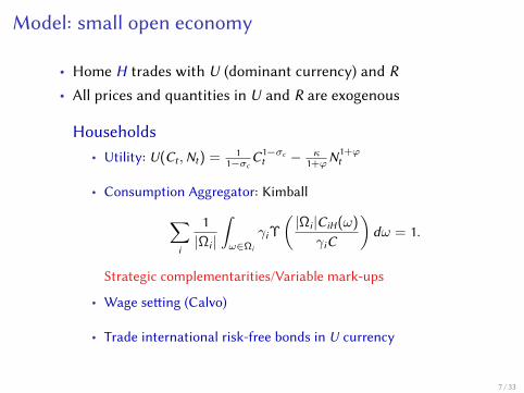
Dominant Currency ParadigmA New Model for the Small Open Economy
Camila Casas Federico DıezBanco de la Republica Federal Reserve Bank of Boston
The views expressed in this paper are those of the authors and do not indicate concurrence by other members of the research staor principals of the Board of Governors, the Federal Reserve Bank of Boston, or the Federal Reserve System. The views expressedin the paper do not represent those of the Banco de la Republica or its Board of Directors. All remaining errors are our own.
1 / 33
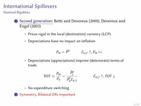
International SpilloversNominal Rigidities
1 First generation (“Consensus View”): Fleming (1962), Mundell(1963), Dornbusch (1976), Svenson & van Wijnbergen (1989), Obstfeld& Rogo (1995)
• Prices rigid in the producer’s currency (PCP)
• Depreciations (appreciations) are inflationary (deflationary)
H Monetary policy shock (25bp cut in policy rate)Γ = 1, α = 0.66, γH = 0.6, η = 1
0 5 10 15 20
#10-3
-2
0
2
4
6
8
10
DCP PCP LCP
(a) ER
0 5 10 15 20
#10-3
-1
-0.5
0
0.5
1
1.5
2
2.5
3
3.5
DCP PCP LCP
(b) π
0 5 10 15 20
#10-3
-2
0
2
4
6
8
10
12
14
DCP PCP LCP
(c) Output
0 5 10 15 20
#10-3
-8
-6
-4
-2
0
2
4
6
8
DCP PCP LCP
(d) TOT12 / 33
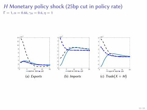
H Monetary policy shock (25bp cut in policy rate)Γ = 1, α = 0.66, γH = 0.6, η = 1
0 5 10 15 20
#10-3
-2
0
2
4
6
8
10
12
14
DCP PCP LCP
(a) Exports
0 5 10 15 20
#10-3
-5
-4
-3
-2
-1
0
1
2
3
4
DCP PCP LCP
(b) Imports
0 5 10 15 20-3
-2
-1
0
1
2
3
4
5#10-3
DCP PCP LCP
(c) Trade(X + M)
13 / 33
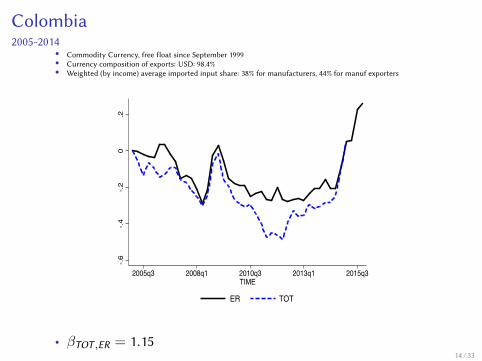
Colombia2005-2014
• Commodity Currency, free float since September 1999• Currency composition of exports: USD: 98.4%• Weighted (by income) average imported input share: 38% for manufacturers, 44% for manuf exporters
-.6-.4
-.20
.2
2005q3 2008q1 2010q3 2013q1 2015q3TIME
ER TOT
• βTOT ,ER = 1.1514 / 33
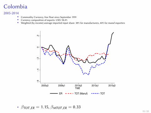
Colombia2005-2014
• Commodity Currency, free float since September 1999• Currency composition of exports: USD: 98.4%• Weighted (by income) average imported input share: 38% for manufacturers, 44% for manuf exporters
-.6-.4
-.20
.2
2005q3 2008q1 2010q3 2013q1 2015q3TIME
ER TOT (Manuf) TOT
• βTOT ,ER = 1.15, βMTOT ,ER = 0.3315 / 33
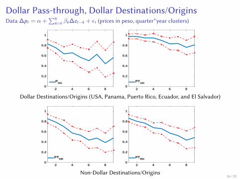
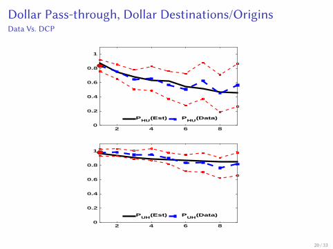
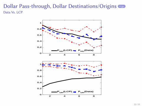
Dollar Pass-through, Dollar Destinations/OriginsData ∆pt = α +
∑8k=0 βk∆et−k + εt (prices in peso, quarter*year clusters)
2 4 6 80
0.2
0.4
0.6
0.8
1
PHU
2 4 6 80
0.2
0.4
0.6
0.8
1
PTUH
Dollar Destinations/Origins (USA, Panama, Puerto Rico, Ecuador, and El Salvador)


![Integrating Human-Computer Interaction Development into ... · paradigm is typically dominant [Hirschheim and Klein, 1989]. For example, the traditional structured approach is within](https://static.documents.pub/doc/80x56/5e9da1f2111da33d79475d90/integrating-human-computer-interaction-development-into-paradigm-is-typically.jpg)


