reflect the positions of the Department of Economics or the University of Notre Dame. Short
sections of text may be quoted without permission provided proper citation is given.
1
Are Long-term Wage Elasticities of Labor Supply More Negative than Short-term Ones?
Kirk Bennett Doran* University of Notre Dame
August, 2012
Abstract
A fundamental prediction of inter-temporal labor supply theory is that the wage-elasticity of labor supply must be more negative the longer the wage change lasts. This paper analyzes labor supply using unique data on workers who choose their own daily hours and who experience both short-term and long-term wage changes. Workers decrease their daily hours in response to short-term wage increases, but not in response to a 20% long-term wage increase. This is consistent with a specific daily income goals model: one in which these goals remain unadjusted to unexpected short-term wage fluctuations, but fully adjust to expected longer-term wage fluctuations. * Email: [email protected] Address: 438 Flanner Hall, University of Notre Dame, Notre Dame, IN 46556
2
I. Introduction
Consider the following thought experiment. A person is offered a wage of one million
dollars an hour to do extremely uninteresting work for the next 24 hours only, after which this
offer expires forever; how many hours would this person prefer to work? Almost all individuals
will respond with a full 24 hours of work for the duration of this short experiment, redistributing
their leisure and sleep to other times. Now suppose that the experiment is extended: the person is
offered a wage of one million dollars an hour to do uninteresting work for every hour of the rest
of their life; how many hours would they prefer to work? All individuals will respond with
much less than 24 hours of work per day, and most would respond with less than a traditional 40
hour work week. This thought experiment is an extreme case of a more general prediction of
standard labor supply theory: the wage-elasticity of labor supply with respect to any wage
change should always be more negative the longer the wage change lasts. This general
prediction has been an essential component to ongoing debates on macroeconomic policy.
In spite of the enormous body of work in labor supply estimation, and in spite of the
importance of such estimation for public economics, macroeconomics, and personnel economics,
several empirical difficulties have prevented this prediction from being tested. First, most hourly
workers must choose their hours within strict contractually-imposed boundaries. Second, there is
likely to be significant heterogeneity across individuals in labor supply behavior, so it is
insufficient to compare short-term wage changes faced by one group of individuals to long-term
wages faced by a different group of individuals. Finally, very long-term wage changes are not
producible in laboratories or field experiments, being outside the time scale of most experimental
budgets. This paper uses a unique data set to address each of these difficulties at the same time:
I collected a panel data set of several months of hour-by-hour work stopping decisions of
3
individual workers who choose their own daily hours. These workers experienced both short-
term fluctuations in earnings opportunities lasting on the order of a day or less, and an
exogenous long-term increase in their hourly wages.
I find that the wage-elasticity of daily labor supply with respect to short-term wage
changes lasting a day or less is approximately -0.25. The wage-elasticity of daily labor supply
with respect to a permanent wage increase is approximately 0.05. The difference in these
elasticities is significantly different from zero, but the sign is in the opposite direction to the
standard prediction: the permanent wage change produces a more positive elasticity than does a
short-term wage change.
I consider the results in light of three broad models of labor supply: (1) the standard inter-
temporal labor supply model; (2) more recent behavioral models of labor supply in which
workers have daily income goals and desire to stop working soon after reaching these goals; and
(3) behavioral models of labor supply in which the daily income goals are rationally determined
in response to expectations about prevailing wage rates. The first model can explain the small
positive elasticity in response to the long-term wage increase, but does not offer a convincing
explanation of the decrease in daily hours in response to short-term wage increases. In
particular, in the standard inter-temporal labor supply model, the elasticity from the long-term
wage increase must be more negative than the elasticity from the short-term ones; and the
elasticity from very short-term wage increases can never be negative. The second model can
explain the decrease in daily hours in response to short-term wage increases, but would predict a
strong decrease in daily hours in response to the large long-term wage increase as well. But the
third model, in which the daily income goals adjust to the long-term wage increase, can explain
both a large negative wage elasticity for short-term wage changes and the lack of a more
4
negative wage elasticity for long-term wage changes. Thus, these results confirm the intuition of
the expectations-based behavioral labor supply theory introduced in Kőszegi and Rabin (2006).
But this explanation of the results raises another question: why did the daily income goals
adapt completely to the long-term wage increase but adapt insufficiently to the short-term wage
fluctuations that lasted one day or less? In fact, the literature on the relationship between effort
and wages has begun to hypothesize that the expectations that determine worker’s targets may
take time to develop, and that high-frequency wage changes may thus inhibit rational adaptation
of these targets (see Chang & Gross (2012)).
The dataset that I introduce in this paper has unique advantages over those used
elsewhere. I introduce a new panel data set of New York City taxi drivers, observing each labor
supply decision after each trip throughout each day in my sample, over a period as long as
several months per driver. I choose taxi drivers so that that I can observe their personally
optimal number of daily hours of work in response to their earnings opportunities: since taxi
drivers can choose their own hours in each 12 hour shift, their labor supply responses are less
likely to be muted by the constraints on working hours common to other occupations. But most
importantly, this data spans a permanent exogenous 26% fare increase instituted by the New
York City Taxi and Limousine Commission on May 3rd, 2004. Thus, this data combines the
benefits of observing the actual decisions of non-hours-constrained workers in the field, with the
benefit of having both very short-term and very long-term wage variation faced by the same
workers.
5
II. A Simple Model of Labor Supply
Suppose that an individual faces T periods of life. Her utility is derived from
consumption of goods and leisure . In each period she faces a wage , and she can save for
future periods at an interest rate . In the general case, her utility allows consumption in one
period to arbitrarily affect her marginal utility of consumption ( ) in any other period;
this is uninteresting, and results in few testable predictions. If, however, we discipline the model
by specifying that her utility is additively separable across periods, then the model makes firm
predictions that have proven useful to both policy makers and economic theorists.
For simplicity, suppose that she faces 2 periods of life, and that her utility can be written:
Her consumption is denoted by , while her labor is denoted by . The wage in period 1 is
, and the wage in period 2 is . Thus, is a scaling factor common to both periods.
The elasticity of substitution across labor between periods is .
It is easy to show that the long-term elasticity (the elasticity of labor supply in period 2
with respect to a change in ) must be more negative than the short-term elasticity (the
elasticity of labor supply in period 2 with respect to a change in ):
Since is a positive constant, and the wages are always positive, it follows that . What
drives this result is not the assumption of 2 periods, but rather the assumption that utility is
additively separable: the consumption in one period cannot affect the marginal utility of
consumption in another period. In this case, a change in one periods’ wage has a smaller
“income effect” than that of the same change in both period’s wages. In other words, the
6
marginal utility of wealth is affected more and more the longer the period of time during which
the wage change occurs.
This result has been central to policy debates within macroeconomics over the last
several decades. It is difficult to test for reasons outlined in the introduction; in particular, since
either short-term or long-term elasticities likely vary greatly between different populations, it is
essential to keep the individual-specific determinants of labor supply constant by considering one
population that has faced both short and long-term wage changes.
III. Short-term Earnings Shocks
The prediction above can be tested by comparing the effects of short-term wage shocks to
those of long-term wage shocks, holding the other determinants of labor supply (specifically the
individual effect) constant. The dataset on taxi drivers that I introduce in this paper provides a
unique opportunity to perform this test. It combines the short-term wage variation common to
other samples of taxi drivers used in the existing literature with an exogenous long-term wage
change that is unique to this data. I describe the short-term wage variation below.
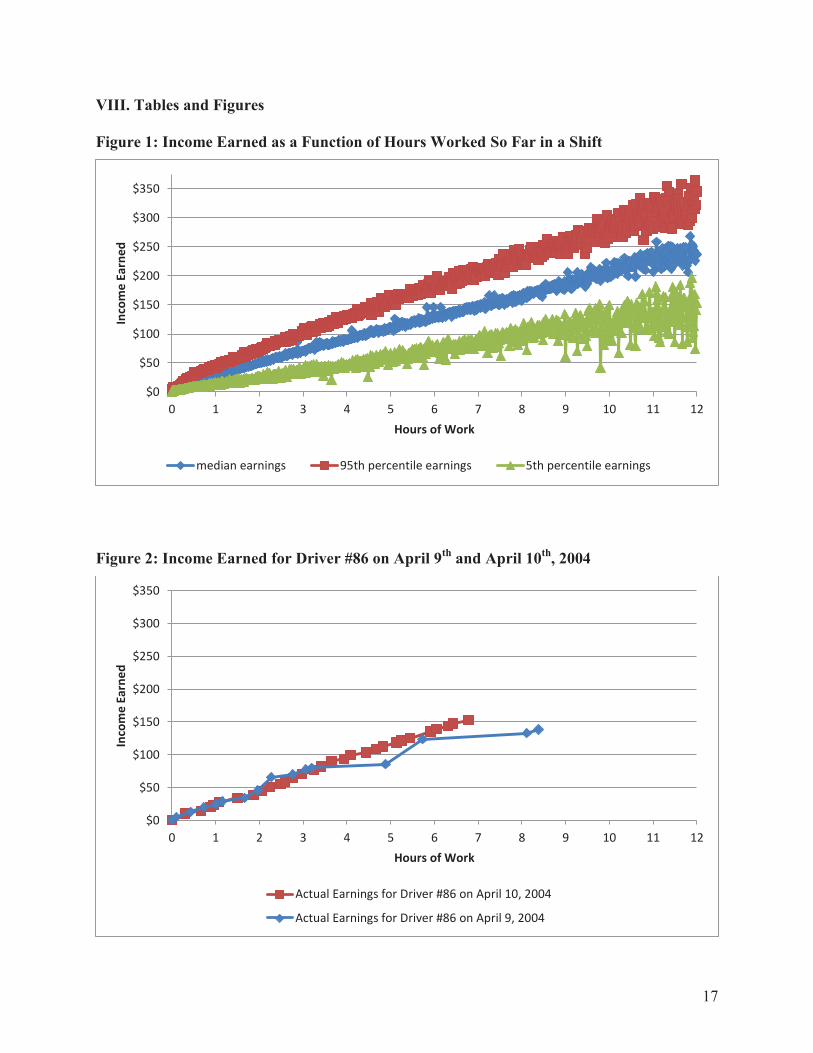
Throughout each shift of work, taxi drivers face varying arrival rates of passengers
hailing cabs. Thus, the income earned by a taxi driver after any number of hours of work can
vary greatly. This can be seen clearly in the novel data set which I introduce in this paper,
consisting of 7,449 taxi driver trip sheets (each covering one shift of work) comprising 155,812
trips. 1 Taking the hours of work and earnings information from these trip sheets, Figure 1 plots
the median earnings, 95th percentile earnings, and 5th percentile earnings as a function of the
number of hours of work they have worked so far in each shift. Clearly, there is wide variation
1 I explain the data in more detail in the data appendix. I report summary statistics in Table 1.
7
in how long it takes to make, for example, $150. A typical day would require about 7 hours of
work to obtain $150 in earnings, but a very good day could achieve $150 in only 5 hours. In
Figure 2, I plot the actual earnings of driver #86 on April 9, and April 10th 2004. There is
variation in earnings opportunities both during the day and across days: on April 9th, this driver
experienced much faster earnings per hour at some parts of his shift than others; and on April
10th, this driver experienced much faster earnings per hour throughout the day than he did on
April 9th.
After each trip is completed, the taxi driver faces a decision of whether to continue
looking for fares or to stop working and go home. What impact, if any, does a faster arrival rate
of income have on the decision to continue working? An individual driver’s labor supply
decision at each potential stopping point can be estimated by a regression where the dependent
variable is the probability of stopping work after any trip, and the independent variables are daily
income earned so far, daily hours worked so far, and the characteristics of the current shift,
current day of the week, and current time of the day.2 Because daily income earned so far is not
perfectly tied down by daily hours worked so far (as Figure 1 shows), both variables can
compete in the same regression as explanations of the probability of stopping work for the day.
Thus, I can make use of the strategy introduced by Farber (2005), and estimate the
where i indexes shifts, and j indexes the trips within each shift. The variable Stop equals 1 if the
driver stops working after this trip and ends his shift, and equals 0 otherwise. Depending on the
2 In particular, it would be a probit regression assuming that there is also a random component of the difference in utilities between going home and continuing to work, and that this random component is distributed normally about 0.
8
specification, Income equals either the income made so far in this shift in dollars (divided by
$20, to make the scaling between income and hours similar), or a set of ten indicator variables
for different levels of income. The variable TimeWorked is a set of controls for the number of
hours worked so far: either the number of hours, the log of the number of hours, or ten indicator
variables. Depending on the specification, the other controls are indicators for the number of
trips made so far, the hour of the day, the day of the week, the month of the year, and whether or
not this shift is a day shift. I also include driver fixed effects in every specification in which I
include multiple drivers, and in such specifications I check the robustness to driver-level
heteroskedasticity through clustering the standard errors at the driver level.
Table 2 reports the results from probit regressions of Equation 1. Regardless of the
specification, the income earned so far during a shift has a positive and significant impact on the
probability of stopping work after the current trip.
I develop an intuitive sense for the magnitude of these positive and significant income
coefficients by considering the following thought experiment: suppose that the drivers noticed
upon entering their cab at the start of their shift that an anonymous donor had gifted them with a
$20 bill, left on the driver’s seat. On average, how would this windfall affect their behavior?
For this calculation, I assume that, ceteris paribus, any individual driver is equally likely
to stop after the first trip as he is after any other trip. I then use the average number of trips per
shift to calculate the base stopping probability after any trip. The coefficient of daily income (a
) from Table 2 determines the effect on the base stopping probability of an extra $20 of income
at the start of the shift.
I then calculate the change in the expected number of trips caused by the increased
stopping probability. Finally, I multiply the change in the expected number of trips by the mean
9
fare per trip to obtain the predicted change in revenue per shift on days in which an extra $20
was dropped in the cab. According to specification (3) reported in Table 2, the drivers would
end the day with only $15.10 extra if they started with $20 dropped on their seat (i.e., on
average, they would earn $4.90 less from their actual work than they otherwise would have).
The implied elasticity of labor supply is obtained by dividing the decrease in earnings by the $20
gift; it is -0.25, with a standard error of 0.05 (the standard error is obtained via the delta method).
This effect persists when I estimate equation 1 separately for each driver.3 I find that 31
out of 66 drivers have positive and significant income coefficients. The average of their implied
elasticities (using each driver’s individual trip statistics in the calculation), is -0.77. This means
that on average these drivers would end the day with only $4.65 extra if they started with $20
dropped on their seat (i.e., on average, they earn $15.35 less from their actual work than they
otherwise would have).
IV. A Long-Term Wage Shock
Do the drivers have a more negative wage-elasticity with respect to a longer-term wage
shock? I can investigate this easily, because my data set spans an important exogenous event: on
May 3rd, 2004 a higher fare for taxis was implemented by the New York City Taxi and
Limousine Commission. The initial charge (called a "fare drop") increased from $2.00 to $2.50,
and the per mile charge increased from $1.50 to $2.00 (Schaller 2006). In addition, a $1
surcharge was added for trips between 4:00pm and 8:00 pm, and during 2004 the flat fare from
3 I estimate a version of Equation 1 for the 66 drivers for whom I have 500 or more observations. Only 2 drivers would be added if I lowered the cutoff to 400 trips, and only 5 dropped if I raised it to 1000.
10
JFK airport to Manhattan was increased from $35 to $45 (Schaller 2006). The cumulative effects
of these fare changes on fares can be seen in Figure 5. The mean fare increased by 26%.
Figures 3 and 4 show that the exogenous wage increase was significant and that it
occurred during a period in which there were no other wage trends and no other daily work hours
trends. But they also show that this large wage increase had no impact on daily hours of work on
average. This is in great contrast to the results for short-term daily earnings shocks, in which
greater daily income significantly reduced the propensity for continuing work for many drivers.
I report in Table 3 the responses of these drivers’ hourly wages, daily hours, and daily
income to the May 2004 fare increase, obtained from OLS regressions of the logs of these
dependent variables on an indicator for the high fare. It is clear that these drivers experienced an
18% hourly wage increase (see Figure 6) and responded with an (insignificant) 2% change in
hours of work per day (the distribution of hours of work per day remained constant, as shown in
Figure 7), resulting in a 20% increase in daily income (see Figure 8). This implies an
(insignificant) wage-elasticity of hours of work of 0.05, with a standard error of 0.10 (obtained
by the delta method).
These results do not change when I restrict the sample to those drivers who "cared" about
daily income according to the individual driver-level regressions reported at the end of Section
III. Even though these drivers had on average a very negative short-term elasticity of -0.77, their
long-term elasticity was still about 0.08.
V. Comparison with Other Estimated Elasticities
The existing literature on workers who can choose their own hours has used other
samples of workers to estimate the short-term wage elasticity of labor supply (see Camerer et al.
11
(1997); Chou (2002); and Farber (2005)) as well as the long-term wage elasticity of labor supply
(see Ashenfelter, Doran, and Schaller (2010)). Comparing a short-term elasticity gleaned from
one sample of workers to a long-term elasticity gleaned from another sample of workers has the
disadvantage of not holding constant the individual-level effects on labor supply decisions.
However, it is worth noting that the estimates from this literature confirm that the long-term
elasticity is not generally more negative than the short-term elasticity.
Camerer et al. (1997) use several different samples of taxi drivers, estimating linear
regressions to obtain estimates of the short-term elasticity which vary between -1.3 to 2.2; the
weighted average of their estimates is -0.75. Chou (2002) uses a sample of taxi drivers from
Singapore to obtain estimates of the short-term elasticity which vary between -1.1 and -0.1; the
weighted average of the estimates is -0.6. Later estimates by Farber (2005) use a still different
sample of taxi drivers and are based on a probit stopping regression that corrects for division
bias; these arrive at an implied elasticity of -0.39, with a standard error of 0.50. Thus, the other
estimates of the short-term wage elasticity on different samples of workers are consistent with
the -0.25 that I report here; and in particular, none of these estimates are more positive than the
0.05 which I report for the long-term elasticity.
Ashenfelter, Doran, and Schaller (2010) use another sample of taxi drivers who own their
own medallions and estimate a long-term labor supply elasticity of -0.20 in response to
permanent wage increases. Neither the estimate of the short-term labor supply elasticity in this
paper, nor the other estimates of the short-term elasticity listed above are more positive than -
0.20.
The explanation which I advance in this paper for the fact that the short-term labor supply
elasticity for wage changes that last less than one day tends to be more negative than the long-
12
term labor supply elasticity for permanent wage changes is the following: workers face income
targets; these income targets adjust to the expected level of wages; and this adjustment takes
longer than a day and less than ten weeks. It is worth asking whether evidence from the
surrounding literature can suggest a tighter bound for the amount of time it takes wage
expectations to adjust (with the caveat that this evidence of course does not come from the same
sample used in this paper).
In fact, Fehr and Goette (2007) estimate a medium-term labor supply elasticity in which
the wages increased for four weeks before they returned to normal; they report that this elasticity
is greater than 1.4 This is more positive than either the long-term elasticity which I have
estimated on this sample, or the long-term elasticity reported in Ashenfelter, Doran, and Schaller
(2010). This suggests that the period of expectations adjustment takes longer than a day and less
than four weeks. Furthermore, this suggests that – apart from very short-term wage changes – the
prediction of the standard labor supply model is confirmed: the wage elasticity of labor supply
indeed becomes more negative as the duration of the wage change increases from four weeks
long to permanent, just as the standard model predicts. In other words, it is only for very short-
term wage changes, that the startling reversal of the standard prediction holds.
VI. Conclusion
Understanding how the hours of labor supplied vary in response to wages is a key input
to debates in public finance, macroeconomics, and personnel economics. But several difficulties
have impeded progress. First, most hourly workers must choose their hours within strict
4 Fehr and Goette document reference dependent effects during their medium-term experiment as well, but these are on effort, not on labor supply itself. For related work, see Gill and Prowse (2012); Pope and Schweitzer (2011); and Abeler, Falk, Goette, and Huffman (2011).
13
contractually-imposed boundaries. Second, there is likely to be significant heterogeneity across
individuals in labor supply behavior. Third, each individual is likely to have different responses
to wage changes that last different periods of time. This paper uses a unique data set to address
each of these difficulties at the same time: the workers in this data had unconstrained hours; they
made a sufficient number of daily labor supply decisions to allow estimation of individual
heterogeneity; and they experienced both short-term fluctuations in earnings opportunities lasting
less than a day, and an exogenous long-term increase in their hourly wages. I find that many
workers decrease their daily hours in response to short-term wage increases that last less than a
day. But, their distribution of daily hours is completely unaffected by a 20% long-term wage
increase; this constancy is true even for those workers whose daily hours were highly affected by
short-term wage increases.
I consider these results in light of three broad models of labor supply: (1) the standard
inter-temporal labor supply model; (2) more recent behavioral models of labor supply in which
workers have daily income goals and desire to stop working soon after reaching these goals, such
as that introduced in Tversky and Kahneman (1991) and analyzed in Camerer, Babcock,
Lowenstein, and Thaler (1997); and (3) behavioral models of labor supply in which the daily
income goals are rationally determined in response to expectations about prevailing wage rates,
such as that introduced in Section V of Kőszegi and Rabin (2006).
The first model can explain the constancy of daily hours of work in response to the long-
term wage increase, but does not offer a convincing explanation of the decrease in daily hours in
response to short-term wage increases. Indeed, the first model would be much more likely to
predict a negative elasticity for the long-term wage increase than the short-term ones, since only
the long-term wage increase has an income effect. The second model can explain the decrease in
14
daily hours in response to short-term wage increases, but would predict a strong decrease in daily
hours in response to the large long-term wage increase as well. But the third model, in which the
daily income goals adjust to the long-term wage increase, can explain both a large negative wage
elasticity for short-term wage changes and the lack of a large negative wage elasticity for long-
term wage changes, as Proposition 4 of Kőszegi and Rabin shows (2006). Thus, these results
confirm the intuition of the expectations-based behavioral labor supply theory.
These results begin to open up the black box of expectations formation in daily income
targets. But they also suggest that for the kind of wage variation that most workers experience –
slow and relatively predictable – daily income goals may not produce the startlingly negative
daily labor supply elasticities that previous research has hypothesized. In conjunction with the
existing literature on workers who can choose their own hours (Fehr and Goette (2007)), these
results provide the first empirical evidence from non-hours-constrained workers that – apart from
very short-term wage changes – the wage elasticity of labor supply does decrease as the duration
of the wage change increases, just as one of the firmest conclusions of the standard labor supply
model predicts. Therefore, it appears that the weaknesses of the standard model are around the
edges, for very short-term wage changes; and these weaknesses are adequately repaired by the
model of expectations-based income targeting introduced by Kőszegi and Rabin (2006), as long
as expectations take longer to adjust than one day of work.
15
VII. References
Abeler , Johannes & Armin Falk & Lorenz Goette & David Huffman. "Reference Points and
Effort Provision," American Economic Review, vol. 101(2), pages 470-92, April 2011.
Ashenfelter, Orley & Kirk Doran & Bruce Schaller. "A Shred of Credible Evidence on the Long-
run Elasticity of Labour Supply," Economica, vol. 77(308), pages 637-650, October
2010.
Camerer, Colin; Linda Babcock; George Lowenstein; and Richard Thaler, “Labor Supply of
New York City Cabdrivers: One Day at a Time,” Quarterly Journal of Economics, May
1997.
Chang, Tom and Tal Gross. “How Many Pears Would a Pear Packer Pack if a Pear Packer Could
Pack Pears at Quasi-Exogenously Varying Piece Rates? An Empirical Evaluation of
Inter-temporal Labor Supply,” mimeo, Columbia University, May, 2012.
Chou, Yuan. “Testing Alternative Models of Labor Supply: Evidence from Cab Drivers in
Crawford, Vincent P. & Juanjuan Meng. "New York City Cab Drivers' Labor Supply Revisited:
Reference-Dependent Preferences with Rational-Expectations Targets for Hours and
Income," American Economic Review, vol. 101(5), pages 1912-32, August 2011.
Farber, Henry S. “Is Tomorrow Another Day? The Labor Supply of New York City Cab
Drivers,” Journal of Political Economy 113 (February 2005).
Farber, Henry S. “Reference-Dependent Preferences and Labor Supply: The Case of New York
City Taxi Drivers,” American Economic Review, 98(3): 1069–82, 2008.
Fehr, Ernst and Lorenz Goette. “Do Workers Work More if Wages Are High? Evidence from a
Randomized Field Experiment,” American Economic Review, Vol. 97, No. 1, Mar., 2007.
16
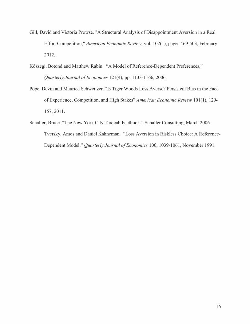
Gill, David and Victoria Prowse. "A Structural Analysis of Disappointment Aversion in a Real
Effort Competition," American Economic Review, vol. 102(1), pages 469-503, February
2012.
Kőszegi, Botond and Matthew Rabin. “A Model of Reference-Dependent Preferences,”
Quarterly Journal of Economics 121(4), pp. 1133-1166, 2006.
Pope, Devin and Maurice Schweitzer. “Is Tiger Woods Loss Averse? Persistent Bias in the Face
of Experience, Competition, and High Stakes” American Economic Review 101(1), 129-
157, 2011.
Schaller, Bruce. “The New York City Taxicab Factbook.” Schaller Consulting, March 2006.
Tversky, Amos and Daniel Kahneman. “Loss Aversion in Riskless Choice: A Reference-
Dependent Model,” Quarterly Journal of Economics 106, 1039-1061, November 1991.
17
VIII. Tables and Figures
Figure 1: Income Earned as a Function of Hours Worked So Far in a Shift
Figure 2: Income Earned for Driver #86 on April 9th
and April 10th
, 2004
$0
$50
$100
$150
$200
$250
$300
$350
0 1 2 3 4 5 6 7 8 9 10 11 12
Inco
me
Ea
rne
d
Hours of Work
median earnings 95th percentile earnings 5th percentile earnings
$0
$50
$100
$150
$200
$250
$300
$350
0 1 2 3 4 5 6 7 8 9 10 11 12
Inco
me
Ea
rne
d
Hours of Work
Actual Earnings for Driver #86 on April 10, 2004
Actual Earnings for Driver #86 on April 9, 2004
18
Figure 3: Mean Earnings per Hour from January 2004 through June 2004
Notes: The exogenous wage increase occurred at the start of the 19th calendar week of 2004. The 95% confidence interval of each 2-week-period’s mean wages shown in error bars.
Figure 4: Mean Hours of Work per Day from January 2004 through June 2004
Notes: The exogenous wage increase occurred at the start of the 19th calendar week of 2004. The 95% confidence interval of each 2-week-period’s mean daily hours in error bars.
Figure 6: Density of Earnings per Hour (Hourly Wage):
0
.05
.1.1
5.2
0 5 10 15 20 25fare per trip ($)
low fare
high fare
kernel = epanechnikov, bandwidth = 1
0
.01
.02
.03
.04
.05
0 20 40 60 80wage ($/hour)
low fare
high fare
kernel = epanechnikov, bandwidth = 1.07
20
Figure 7: Density of Hours of Work per Shift:
Figure 8: Density of Income Earned per Shift:
0
.05
.1.1
5
0 5 10 15 20 25hours per shift
low fare
high fare
kernel = epanechnikov, bandwidth = .49
0
.00
2.0
04
.00
6.0
08
0 100 200 300 400 500 600income per shift ($)
low fare
high fare
kernel = epanechnikov, bandwidth = 9.99
21
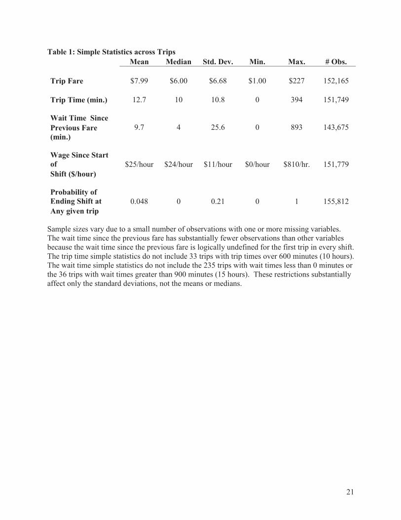
Table 1: Simple Statistics across Trips
Mean Median Std. Dev. Min. Max. # Obs.
Trip Fare $7.99 $6.00 $6.68 $1.00 $227 152,165
Trip Time (min.) 12.7 10 10.8 0 394 151,749
Wait Time Since
9.7 4 25.6 0 893 143,675 Previous Fare
(min.)
Wage Since Start
of $25/hour $24/hour $11/hour $0/hour $810/hr. 151,779
Shift ($/hour)
Probability of
Ending Shift at 0.048 0 0.21 0 1 155,812
Any given trip
Sample sizes vary due to a small number of observations with one or more missing variables. The wait time since the previous fare has substantially fewer observations than other variables because the wait time since the previous fare is logically undefined for the first trip in every shift. The trip time simple statistics do not include 33 trips with trip times over 600 minutes (10 hours). The wait time simple statistics do not include the 235 trips with wait times less than 0 minutes or the 36 trips with wait times greater than 900 minutes (15 hours). These restrictions substantially affect only the standard deviations, not the means or medians.
22
Table 2: Marginal Effects of Daily Income & Hours on Stopping Probability
(estimation of one probit regression over all drivers)
(1) (2) (3) (4)
Income earned so far in $20s 0.004*** 0.002*** 0.001*** --
(0.000) (0.000) (0.000) -- Implied Wage-Elasticity of Daily Hours of Work
-0.65 (0.05)
-0.34 (0.05)
-0.25 (0.05)
Hours worked so far 0.005*** 0.003*** -- --
(0.000) (0.000) -- --
Log of Trips made so far 0.007*** 0.005*** -- --
(0.002) (0.001) -- --
Day Shift Indicator -0.018*** -0.001 -0.002 -0.002
(0.003) (0.003) (0.002) (0.002)
Average effect of $20 income 0.004*** 0.002*** 0.001*** 0.001**
(p-value for joint significance) (0.000) (0.000) (0.000) (0.020) Average effect of hour of work 0.005*** 0.003*** 0.010*** 0.012***
(p-value for joint significance) (0.000) (0.000) (0.000) (0.000)
Income Controls Level Level Level 10 Indicators
Hours worked so far Controls Level Level 10 Indicators 10 Indicators
Trip Controls Log Log 63 Indicators 63 Indicators
Hour of the Day Controls NO 23 Indicators 23 Indicators 23 Indicators
# of Observations 151,761 151,101 151,101 151,101
Pseudo R² 0.20 0.24 0.25 0.25
All regressions include controls for day of the week, month of the year, and driver fixed effects. The average effect of income and the average effect of an hour of work are either the coefficient of each of these variables (in specifications in which they appear as levels), or the slope of a line fit through the ten indicator variables (in specifications in which they are coded as indicator variables). The p-value for joint significance of these variables is either the p-value for the significance of the level (in specifications in which the variables are coded as levels), or the p-value for joint significance of all ten indicator variables (in the flexible specifications). Sample sizes change slightly in each case because some driver and hour of the day indicators occasionally predict failure perfectly and thus must be dropped (with associated observations) in order for the probit regression to run. The hours worked so far controls are jointly significant at the 0.000% level in specification (4). Standard Errors, corrected for driver-level clustering, are in parentheses. The implied short-term elasticity is calculated as explained in Section III; its standard error is obtained through the delta method. * Significant at 10% ** 5% *** 1%
23
Table 3. Effects of 26% Fare Increase
(fixed effects linear regressions)
Panel A. All Drivers
(1) log of Average Hourly Wage in Shift
(2) Log of Total Minutes in Shift
(3) Log of Total Income in Shift
High Fare Indicator (after May 3rd 2004)
0.18*** (0.01)
0.01 (0.02)
0.18*** (0.02)
R^2 0.16 0.28 0.26 # observations 6958 6958 6958 Panel B. Drivers with income goals
(1) log of Average Hourly Wage in Shift
(2) Log of Total Minutes in Shift
(3) Log of Total Income in Shift
High Fare Indicator (after May 3rd 2004)
0.18*** (0.01)
0.01 (0.02)
0.19*** (0.02)
R^2 0.17 0.17 0.16 # observations 3651 3651 3651 An observation is an individual shift of work (trip sheet) by an individual driver. In Panel B, the sample is restricted to shifts worked by drivers with positive and significant coefficients on the cumulative daily income earned so far in a given day in individual-driver-level regressions of stopping probability. All specifications control for the day of the week, the hour of the day, whether the shift is a day shift, and driver-level fixed effects. Standard Errors, corrected for driver-level clustering, are in parentheses. * = Significant at 10%, ** = 5%, *** = 1%
24
IX. Data Appendix
(A) Characteristics of Data
The novel data set I introduce in this paper consists of 7449 taxi driver trip sheets
(each covering one shift of work), comprising 155,812 trips. These shifts were
undertaken by 106 drivers, 84 of whom report more than 100 trips (or about five shifts of
work). A total of 66 drivers report more than 500 trips (or about 25 shifts of work), and
therefore I have a large number of drivers who report working on many days. Over 95%
of the data is from the year 2004, with the remaining from 2003 and 2005. Of the year
2004 data, about 99% is from January through June. I have almost every day of work for
some drivers for several months in a row, resulting in a panel data set that makes possible
estimation that uses income and work decisions across days. Furthermore, my data set
spans an important exogenous event: on May 3rd, 2004 a higher fare for taxis was
implemented by the New York City Taxi and Limousine Commission. I obtained these
trip sheets from an anonymous taxi company in New York City, and the
representativeness of this sample should be similar to that of those used in the papers in
the existing taxi literature (see Camerer et al (1997), Farber (2005), Farber (2008), and
Crawford and Meng (2011)).5
5 During my visits to New York City taxi companies, I observed that as many as half of taxi drivers do not fill out their trip sheets completely. Thus, samples used in the existing literature composed primarily of complete trip sheets must have been obtained from companies that deleted a substantial number of drivers before sharing their sheets. In collecting my sample, I was able to avoid interference by the company, but I was still forced to restrict my sample to drivers who were clearly filling out enough trips per sheet and enough trip sheets per month that, for example, their reported earnings would have been enough to pay their taxi rental fees. In Camerer et al. (1997) the authors deleted 122 incomplete trip sheets from the 192 trip sheets in one of their samples when calculating their main results, though they found that this deletion did not affect outcomes. The
25
(B) Data Reliability
One easy check of the reliability of the data is to make use of the exogenous wage
shift instituted by the New York City Taxi and Limousine Commission on May 3rd, 2004.
The 2006 New York City Taxi Cab Factbook (Schaller 2006) reports that in May 2004,
the initial charge (fare drop) increased from $2.00 to $2.50, and the per mile charge
increased from $1.50 to $2.00 (the waiting time charge stayed roughly constant, and the
per minute charge stayed constant). In addition, in May 2004 a $1 surcharge was added
for trips between 4:00pm and 8:00 pm, and during 2004 the flat fare from JFK airport to
Manhattan was increased from $35 to $45. Calculating the effect of the May 2004 fare
change on a 2.8 mile trip with 4.77 minutes of wait time that does not overlap rush hour
(4:00 pm to 8:00 pm), the Factbook concludes that the fare should have increased from
$6.85 to $8.65, or by about 26%. This gives a rough estimate of the average fare change
I should find in my data.
What I actually find in my data is that the average effect of the May fare increase
(for trips that end before rush hour begins or after rush hour ends) is an increase of $1.93,
with a 95% confidence interval of $1.85 to $2.00. Since the average such fare was $7.06
before the fare change, this represents a precisely measured average fare increase of
27%.6 The precision of this estimate and its closeness with the known change in fare
rules are evidence that the fares that the drivers recorded (and that the research assistants
ultimate solution would be data from electronic meters that cannot be turned off by the drivers. Nonetheless, the distributions in my data match well those independently described by other authors using both other data sets and official fare information. My sample is thus very unlikely to be either more or less representative than those used in the existing published papers in this literature. 6 Restricting the sample to trips that are between 10 and 20 minutes in length (in an attempt to more closely replicate the waiting time of 4.77 minutes and length of 2.8 miles from the thought experiment) leads to a precisely-measured 23% wage increase.
26
observed and entered into the computer) correspond with reality: it would be unlikely that
the drivers could replicate this fare change if they were inventing the fares that they wrote
down. The effects of the fare change on overage fares and on average hourly wages are
reported in Figure 1, Figure 2, and Figure 3.
Furthermore, the representativeness of this sample is supported by the fact that the
simple statistics I describe below match well the simple statistics from other independent
samples collected and described by the other authors in the taxi literature.
(C) Simple Statistics
In Table 1, I report simple statistics at the trip level. It is clear that most trips are
short (median time is 10 minutes), with small fares (median fare is $6.00) and that the
wait time between trips is often very short (median wait time is 4 minutes). In addition,
after any trip the average probability of stopping work for the day is quite low: 4.8%.
According to the shift-level statistics in Figures 4 and 5, drivers typically earn about $160
a shift, after working for almost eight hours on average.
(D) Drivers without enough observations
In specifications in which I estimate separate labor supply functions for each
driver, I must restrict myself to drivers with a sufficient number of observations to make
this estimation possible. Given the large number of independent variables in each
equation, I thus make use of drivers with 500 or more total trips in the sample. This
restricts me to 66 drivers out of the original 106.7
7 Only 2 drivers would be added if I lowered the cutoff to 400 trips, and only 5 dropped if I raised it to 1000.