Zeph Smith

Salt Lake Community

College Department of Mathematics

4600 S. Redwood Road

SLC, UT 81230

801-957-EBAY

DDDD PPPP

PPPP OOOO RRRR TTTT FFFF

RRRR SSSS

OOOO

TTTT

SSSS LLLL

FFFF OOOO LLLL IIII OOOO

OOOO EEEE

RRRR

Zeph Smith

2009

Zeph Smith

2009-2010

To the Faculty Evaluation Committee March 2010 To assist you in evaluating my effectiveness as an educator, I have included in this dossier the following items:

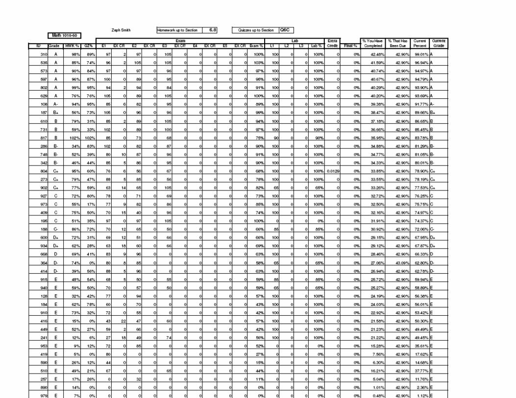
1. An addendum of additional items for consideration in evaluating my teaching effectiveness 2. A copy of each of the 3 Math 1010 projects I developed this year. 3. A copy of the least squares project I designed for Math 1050 4. A copy of a letter of appreciation from a teacher I have been mentoring 5. A copy of a syllabus for one of the classes I taught 6. A copy of the grade sheet that I designed to track student performance. The students in my

classes are given multiple opportunities on a weekly basis to view their current progress and grades, as this has been one of the most positively commented aspects students have given me on how I conduct my classes.

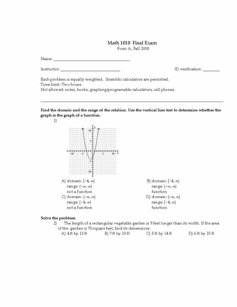
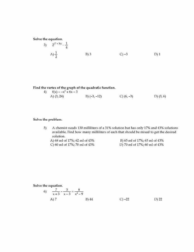
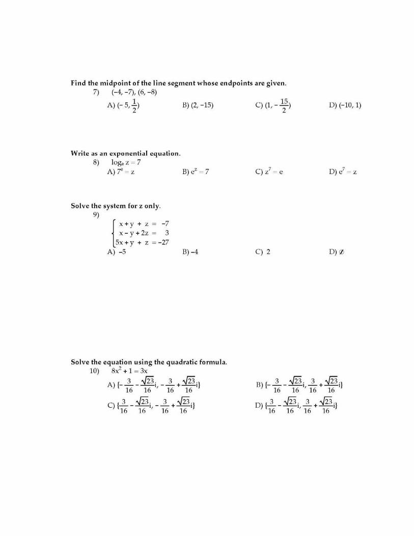
7. A copy of one of the three versions of the Fall 2008 Math 1010 Final I wrote In addition to these submissions I have also included a page illustrating some of the ideas I use in my class to enhance both student learning and effective teaching. As evidence of my service to the college, I

1. Serve as the Course Coordinator for Math 1010 with duties including the creation of the three versions of the departmental final for Fall 2009 and Spring 2010, the creation of online versions of the class for use by students in a live class, and the creation of three new math 1010 level mathematics labs.

2. Serve on four committees charged with the selection of new text books for the Mathematics Department

3. Have served on the Quality Higher Education Council as the SME representative. 4. Have continued to teach overload classes and regular load classes of large enrollment with the

goal of providing excellent education and service to as many students as I can 5. Have mentored adjunct faculty members in getting access and using the online math MML

environment, using Virtual TI, looking over exams, and providing tests and reviews to use. As evidence of my maintaining and developing my knowledge in the Mathematics field, I have:

1. Studied various books on different ways to do basic to intermediate mathematics mentally, ways to do mathematics visually, ways to apply mathematics to the liberal arts, and others.

2. Continued to read modern mathematical textbooks that I currently do not use to gain insights into alternative teaching styles and methods as well as other examples of how community college level mathematics is used in every day life.

3. Participated in Starlink presentations offered by the FTLC as a way to develop myself and my level of teaching expertise to better serve my students.

4. Participated in a Wimba training and demonstration session to better understand how to use Wimba to enhance my courses

Thank you for your consideration. Zeph Smith Instructor Mathematics Salt Lake Community College

Additional items for consideration in evaluating my teaching effectiveness: � One of the methods I use to gather student input on teaching classes is to give each

student a sticky note. I then ask them to answer 5 questions: 1. How does the course enhance your learning? 2. How does the course detract from your learning? 3. How does my teaching enhance your learning? 4. How does my teaching detract from your learning? 5. What else would you like to communicate at this time? I ask them to put the sticky notes on the door on their way out. This way it is anonymous and I get instant feedback. I follow this up with telling the class the overall communication I received from the sticky notes and what I am going to continue to do or do differently in response to their feedback.

� One of the ways I encourage students to learn from their mistakes is to give quizzes

after I hand back tests. A few days after I give them the graded tests, I give them a quiz that consists of 3 problems at random from the test. The questions have slight number changes from those on the test. Based on their performance on this quiz they can receive up to 50% of the missed test points back. For them to have these points applied to their grades, they also have to turn in a key to the test. In this way I have them figure out what mistakes they made, correct them and then demonstrate their knowledge in a testing environment. They also have created a document that they can use for final review.

� One of the methods I have developed recently to ensure student involvement is what I

call “Robo Math.” Starting at a random student, they tell me (the robot) a step to perform on a problem on the board. Then it is the next student’s turn. This person can either use their turn to continue solving the problem, or to undo the last step if they feel it is in the wrong direction. Once the problem is complete, we continue with a new one until everyone has had a chance to have at least one turn. If a student cannot answer during their turn, I tell them that I will come back to them soon with a similar step. I have had a lot of positive response from students about this method. They think it has them pay much better attention in class and think during every step of the problem rather than only listen to whoever is answering.

� Another method I have found useful to get instant feedback is the “high five”. I ask

students to raise fingers to communicate how well they understand the current topic, with 5 being great and a fist being totally confused. If the overall understanding is low, I continue with explanations and demonstrations and ask them again.

� I also like to have my students all respond to a multiple choice question during a

discussion with thumbs up, side or down. This way I can involve all of the students at the same time.

� I have continued to experiment with having students do homework online as a way to

have my students perform better on the final exam. I have split up the homework into different parts so students can get some work done on material before new material is learned, and still have time to finish after more lecture time. My final grade averages have continued to improve with these changes. Online homework is not perfect, but with enough setup, it does positively influence the success rate of my students. I will always be looking for better methods of teaching, practicing, and studying.

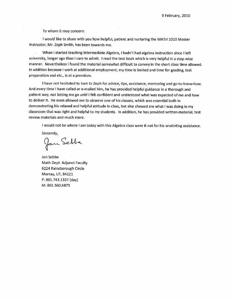
� I have written a few letters of recommendation for past students in the past year.

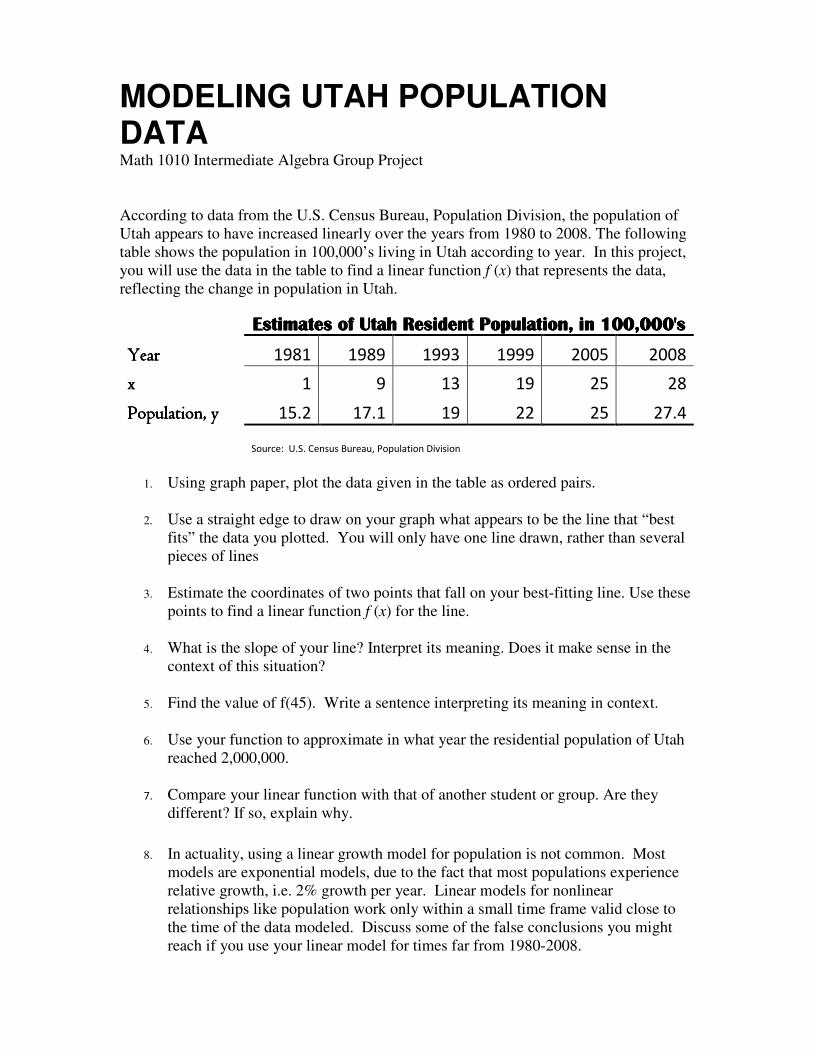
MODELING UTAH POPULATION DATA Math 1010 Intermediate Algebra Group Project According to data from the U.S. Census Bureau, Population Division, the population of Utah appears to have increased linearly over the years from 1980 to 2008. The following table shows the population in 100,000’s living in Utah according to year. In this project, you will use the data in the table to find a linear function f (x) that represents the data, reflecting the change in population in Utah.

Estimates of Utah Resident Population, in 100,000'sEstimates of Utah Resident Population, in 100,000'sEstimates of Utah Resident Population, in 100,000'sEstimates of Utah Resident Population, in 100,000's

YearYearYearYear 1981 1989 1993 1999 2005 2008

xxxx 1 9 13 19 25 28

Population, yPopulation, yPopulation, yPopulation, y 15.2 17.1 19 22 25 27.4

Source: U.S. Census Bureau, Population Division

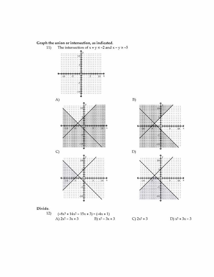
1. Using graph paper, plot the data given in the table as ordered pairs.

2. Use a straight edge to draw on your graph what appears to be the line that “best

fits” the data you plotted. You will only have one line drawn, rather than several pieces of lines

3. Estimate the coordinates of two points that fall on your best-fitting line. Use these points to find a linear function f (x) for the line.

4. What is the slope of your line? Interpret its meaning. Does it make sense in the

context of this situation?

5. Find the value of f(45). Write a sentence interpreting its meaning in context.

6. Use your function to approximate in what year the residential population of Utah reached 2,000,000.

7. Compare your linear function with that of another student or group. Are they

different? If so, explain why.

8. In actuality, using a linear growth model for population is not common. Most models are exponential models, due to the fact that most populations experience relative growth, i.e. 2% growth per year. Linear models for nonlinear relationships like population work only within a small time frame valid close to the time of the data modeled. Discuss some of the false conclusions you might reach if you use your linear model for times far from 1980-2008.

Maximizing the Profit of a Business Math 1010 Intermediate Algebra Group Project In this project your group will solve the following situation: A manufacturer produces the following two items: computer desks and bookcases. Each item requires processing in each of two departments. Department A has 55 hours available and department B has 39 hours available each week for production. To manufacture a computer desk requires 4 hours in department A and 3 hours in department B while a bookcase requires 3 hours in department A and 2 hours in department B. Profits on the items are $72 and $23 respectively. If all the units can be sold, how many of each should be made to maximize profits? Let X be the number of computer desks that are sold and Y be number of bookcases sold.

1. Write down a linear inequality for the hours used in Department A

2. Write down a linear inequality for the hours used in Department B

There are two other linear inequalities that must be met. These relate to the fact that the

manufacturer cannot produce negative numbers of items. These inequalities are as follows:

0

0

X

Y

≥

≥

3. Next, write down the profit function for the sale of X desks and Y bookcases:

P =

You now have four linear inequalities and a profit function. These together describe the manufacturing situation. These together make up what is known mathematically as a linear programming problem. Write all of the inequalities and the profit function together below. This is typically written one on top of another, with the profit function last.

4. To solve this problem, you will need to graph the

on one common XY plane.

origin, with the horizontal axis representing X and the vertical axis representing Y.

To solve this problem, you will need to graph the intersection of all four

on one common XY plane. Do this on the grid below. Have the bottom left be the

origin, with the horizontal axis representing X and the vertical axis representing Y.

of all four inequalities

left be the

origin, with the horizontal axis representing X and the vertical axis representing Y.

5. The above shape should have 4 corners. Find the coordinates of the ordered pairs that

make up these corners. For the intersection of the two slanted lines you will have to

solve the 2 by 2 system made up of their equations.

6. The last thing to do is to plug each of the points you found in part 5 into the profit

function to determine which ordered pair gives the maximum profit. Do this and write a

sentence describing how many of each type of furniture you should build and sell and

what is the maximum profit you will make.

Height of a Zero Gravity Parabolic

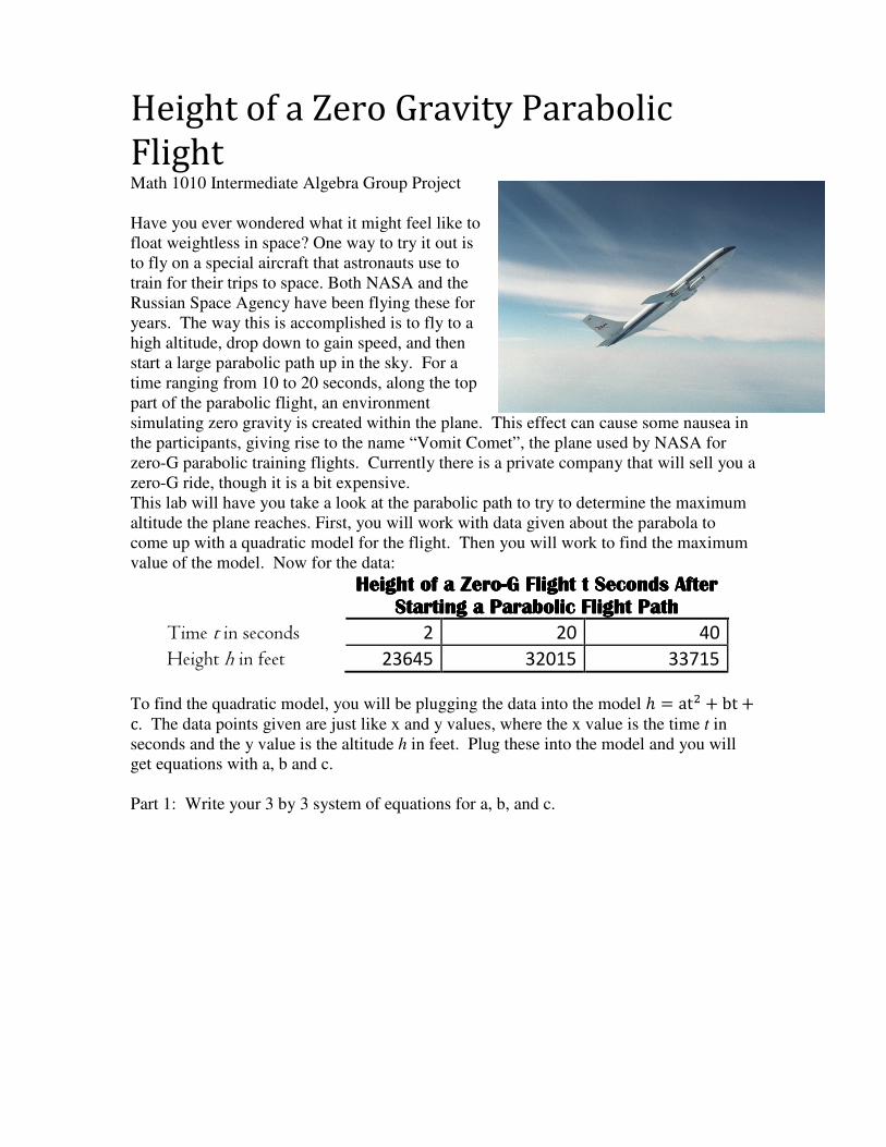
Flight Math 1010 Intermediate Algebra Group Project Have you ever wondered what it might feel like to float weightless in space? One way to try it out is to fly on a special aircraft that astronauts use to train for their trips to space. Both NASA and the Russian Space Agency have been flying these for years. The way this is accomplished is to fly to a high altitude, drop down to gain speed, and then start a large parabolic path up in the sky. For a time ranging from 10 to 20 seconds, along the top part of the parabolic flight, an environment simulating zero gravity is created within the plane. This effect can cause some nausea in the participants, giving rise to the name “Vomit Comet”, the plane used by NASA for zero-G parabolic training flights. Currently there is a private company that will sell you a zero-G ride, though it is a bit expensive. This lab will have you take a look at the parabolic path to try to determine the maximum altitude the plane reaches. First, you will work with data given about the parabola to come up with a quadratic model for the flight. Then you will work to find the maximum value of the model. Now for the data:

Height of a ZeroHeight of a ZeroHeight of a ZeroHeight of a Zero----G Flight t Seconds After G Flight t Seconds After G Flight t Seconds After G Flight t Seconds After

Starting a Parabolic Flight PathStarting a Parabolic Flight PathStarting a Parabolic Flight PathStarting a Parabolic Flight Path

Time t in seconds 2 20 40

Height h in feet 23645 32015 33715

To find the quadratic model, you will be plugging the data into the model � � at�� bt �

c. The data points given are just like x and y values, where the x value is the time t in seconds and the y value is the altitude h in feet. Plug these into the model and you will get equations with a, b and c. Part 1: Write your 3 by 3 system of equations for a, b, and c.

Part 2: Solve this system. Make sure to show your work.

Part 3: Using your solutions to the system from part 2 to form your quadratic model of the data. Part 4: Find the maximum value of the quadratic function. Make sure to show your work.

Part 5: Sketch the parabola. Label the given data plus the maximum point.to start labeling your axes is to have the lower left point be (0, 20000)

Part 5: Sketch the parabola. Label the given data plus the maximum point. to start labeling your axes is to have the lower left point be (0, 20000)

A good way

Linear Least Squares Approximation Lab or Fitting a Polynomial Curve to a Set of Data Points.

Part I Introduction

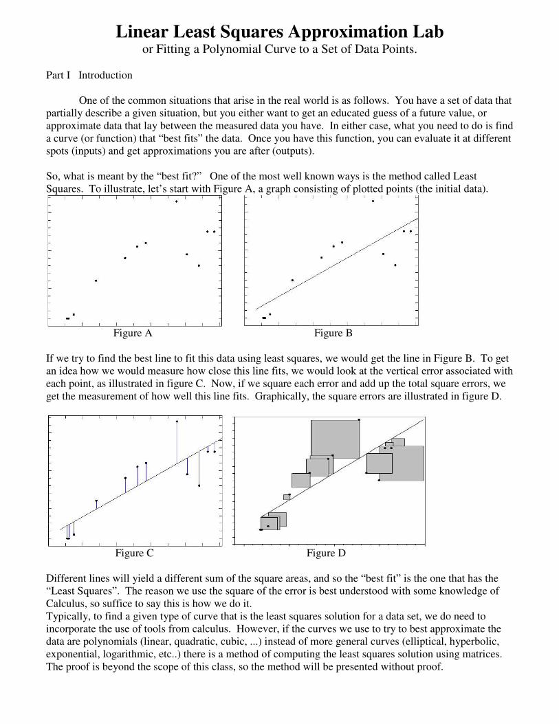
One of the common situations that arise in the real world is as follows. You have a set of data that partially describe a given situation, but you either want to get an educated guess of a future value, or approximate data that lay between the measured data you have. In either case, what you need to do is find a curve (or function) that “best fits” the data. Once you have this function, you can evaluate it at different spots (inputs) and get approximations you are after (outputs). So, what is meant by the “best fit?” One of the most well known ways is the method called Least Squares. To illustrate, let’s start with Figure A, a graph consisting of plotted points (the initial data).

Figure A Figure B If we try to find the best line to fit this data using least squares, we would get the line in Figure B. To get an idea how we would measure how close this line fits, we would look at the vertical error associated with each point, as illustrated in figure C. Now, if we square each error and add up the total square errors, we get the measurement of how well this line fits. Graphically, the square errors are illustrated in figure D.

Figure C Figure D Different lines will yield a different sum of the square areas, and so the “best fit” is the one that has the “Least Squares”. The reason we use the square of the error is best understood with some knowledge of Calculus, so suffice to say this is how we do it. Typically, to find a given type of curve that is the least squares solution for a data set, we do need to incorporate the use of tools from calculus. However, if the curves we use to try to best approximate the data are polynomials (linear, quadratic, cubic, ...) instead of more general curves (elliptical, hyperbolic, exponential, logarithmic, etc..) there is a method of computing the least squares solution using matrices. The proof is beyond the scope of this class, so the method will be presented without proof.

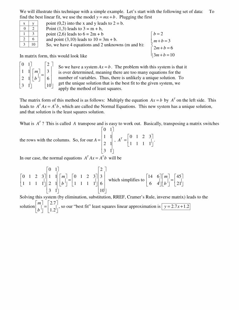
We will illustrate this technique with a simple example. Let’s start with the following set of data: To find the best linear fit, we use the model y mx b= + . Plugging the first

point (0,2) into the x and y leads to 2 = b. Point (1,3) leads to 3 = m + b, point (2,6) leads to 6 = 2m + b and point (3,10) leads to 10 = 3m + b. So, we have 4 equations and 2 unknowns (m and b):

In matrix form, this would look like So we have a system Ax b= . The problem with this system is that it is over determined, meaning there are too many equations for the number of variables. Thus, there is unlikely a unique solution. To get the unique solution that is the best fit to the given system, we apply the method of least squares.

The matrix form of this method is as follows: Multiply the equation Ax b= by TA on the left side. This

leads to T TA Ax A b= , which are called the Normal Equations. This new system has a unique solution,

and that solution is the least squares solution.

What is ?TA This is called A transpose and is easy to work out. Basically, transposing a matrix switches

the rows with the columns. So, for our

0 1

1 1 0 1 2 3,

2 1 1 1 1 1

3 1

TA A

= =

.

In our case, the normal equations T TA Ax A b= will be

0 1 2

0 1 2 3 1 1 0 1 2 3 3

1 1 1 1 2 1 1 1 1 1 6

3 1 10

m

b

=

which simplifies to 14 6 45

6 4 21

m

b

=

Solving this system (by elimination, substitution, RREF, Cramer’s Rule, inverse matrix) leads to the

solution2.7

1.2

m

b

=

, so our “best fit” least squares linear approximation is 2.7 1.2y x= +

x y

0 2

1 3

2 6

3 10

2

3

2 6

3 10

b

m b

m b

m b

=

+ =

+ = + =

0 1 2

1 1 3

2 1 6

3 1 10

m

b

=

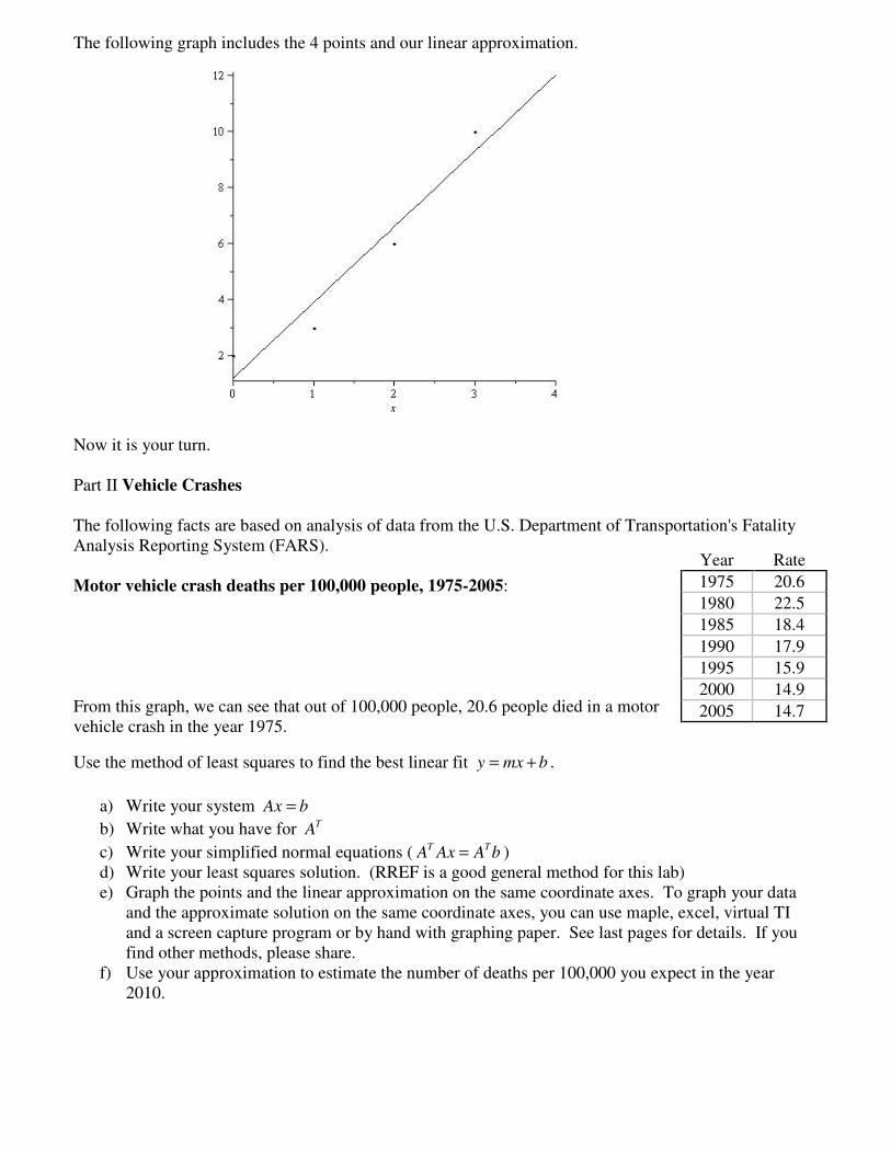
The following graph includes the 4 points and our linear approximation. Now it is your turn. Part II Vehicle Crashes The following facts are based on analysis of data from the U.S. Department of Transportation's Fatality Analysis Reporting System (FARS). Motor vehicle crash deaths per 100,000 people, 1975-2005: From this graph, we can see that out of 100,000 people, 20.6 people died in a motor vehicle crash in the year 1975.

Use the method of least squares to find the best linear fit y mx b= + .

a) Write your system Ax b=

b) Write what you have for TA

c) Write your simplified normal equations ( T TA Ax A b= )

d) Write your least squares solution. (RREF is a good general method for this lab) e) Graph the points and the linear approximation on the same coordinate axes. To graph your data

and the approximate solution on the same coordinate axes, you can use maple, excel, virtual TI and a screen capture program or by hand with graphing paper. See last pages for details. If you find other methods, please share.

f) Use your approximation to estimate the number of deaths per 100,000 you expect in the year 2010.

Year Rate

1975 20.6

1980 22.5

1985 18.4

1990 17.9

1995 15.9

2000 14.9

2005 14.7

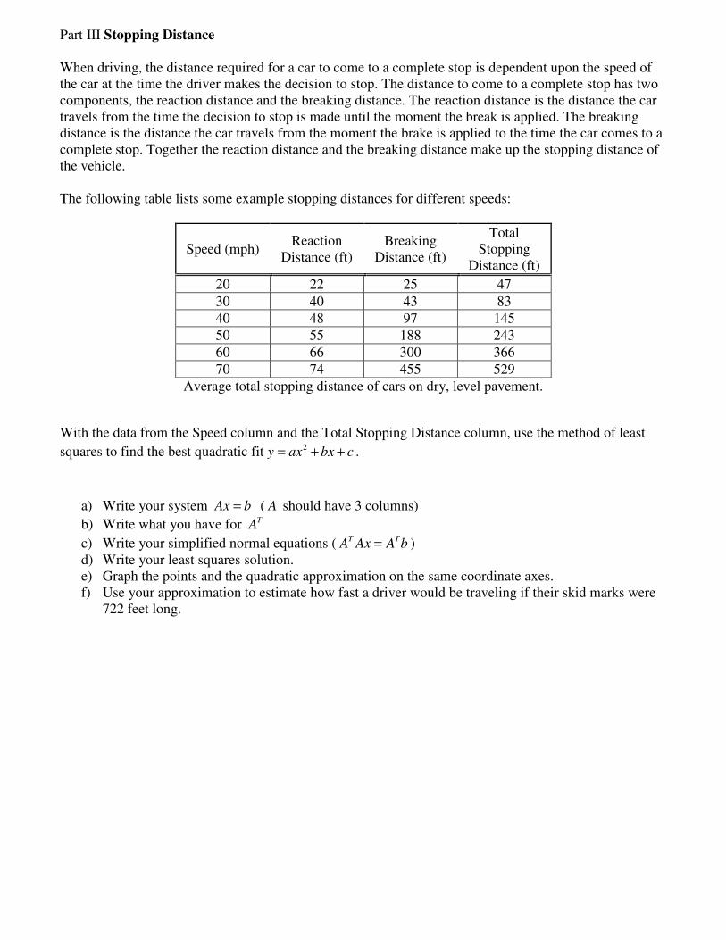
Part III Stopping Distance When driving, the distance required for a car to come to a complete stop is dependent upon the speed of the car at the time the driver makes the decision to stop. The distance to come to a complete stop has two components, the reaction distance and the breaking distance. The reaction distance is the distance the car travels from the time the decision to stop is made until the moment the break is applied. The breaking distance is the distance the car travels from the moment the brake is applied to the time the car comes to a complete stop. Together the reaction distance and the breaking distance make up the stopping distance of the vehicle. The following table lists some example stopping distances for different speeds:

Speed (mph) Reaction

Distance (ft) Breaking

Distance (ft)

Total Stopping

Distance (ft)

20 22 25 47

30 40 43 83

40 48 97 145

50 55 188 243

60 66 300 366

70 74 455 529

Average total stopping distance of cars on dry, level pavement.

With the data from the Speed column and the Total Stopping Distance column, use the method of least

squares to find the best quadratic fit 2y ax bx c= + + .

a) Write your system Ax b= ( A should have 3 columns)

b) Write what you have for TA

c) Write your simplified normal equations ( T TA Ax A b= )

d) Write your least squares solution. e) Graph the points and the quadratic approximation on the same coordinate axes. f) Use your approximation to estimate how fast a driver would be traveling if their skid marks were

722 feet long.

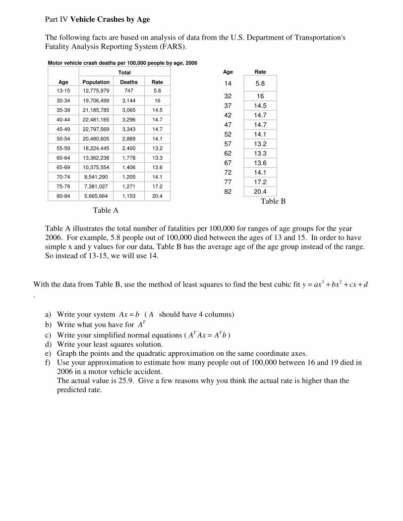
Part IV Vehicle Crashes by Age The following facts are based on analysis of data from the U.S. Department of Transportation's Fatality Analysis Reporting System (FARS).

Motor vehicle crash deaths per 100,000 people by age, 2006

Age Rate

14 5.8

32 16

37 14.5

42 14.7

47 14.7

52 14.1

57 13.2

62 13.3

67 13.6

72 14.1

77 17.2

82 20.4

Table B Table A Table A illustrates the total number of fatalities per 100,000 for ranges of age groups for the year 2006. For example, 5.8 people out of 100,000 died between the ages of 13 and 15. In order to have simple x and y values for our data, Table B has the average age of the age group instead of the range. So instead of 13-15, we will use 14.

With the data from Table B, use the method of least squares to find the best cubic fit 3 2y ax bx cx d= + + +

.

a) Write your system Ax b= ( A should have 4 columns)

b) Write what you have for TA

c) Write your simplified normal equations ( T TA Ax A b= )

d) Write your least squares solution. e) Graph the points and the quadratic approximation on the same coordinate axes. f) Use your approximation to estimate how many people out of 100,000 between 16 and 19 died in

2006 in a motor vehicle accident. The actual value is 25.9. Give a few reasons why you think the actual rate is higher than the predicted rate.

Age

Total

Population Deaths Rate

13-15 12,775,979 747 5.8

30-34 19,706,499 3,144 16

35-39 21,185,785 3,065 14.5

40-44 22,481,165 3,296 14.7

45-49 22,797,569 3,343 14.7

50-54 20,480,605 2,889 14.1

55-59 18,224,445 2,400 13.2

60-64 13,362,238 1,778 13.3

65-69 10,375,554 1,406 13.6

70-74 8,541,290 1,205 14.1

75-79 7,381,027 1,271 17.2

80-84 5,665,664 1,153 20.4

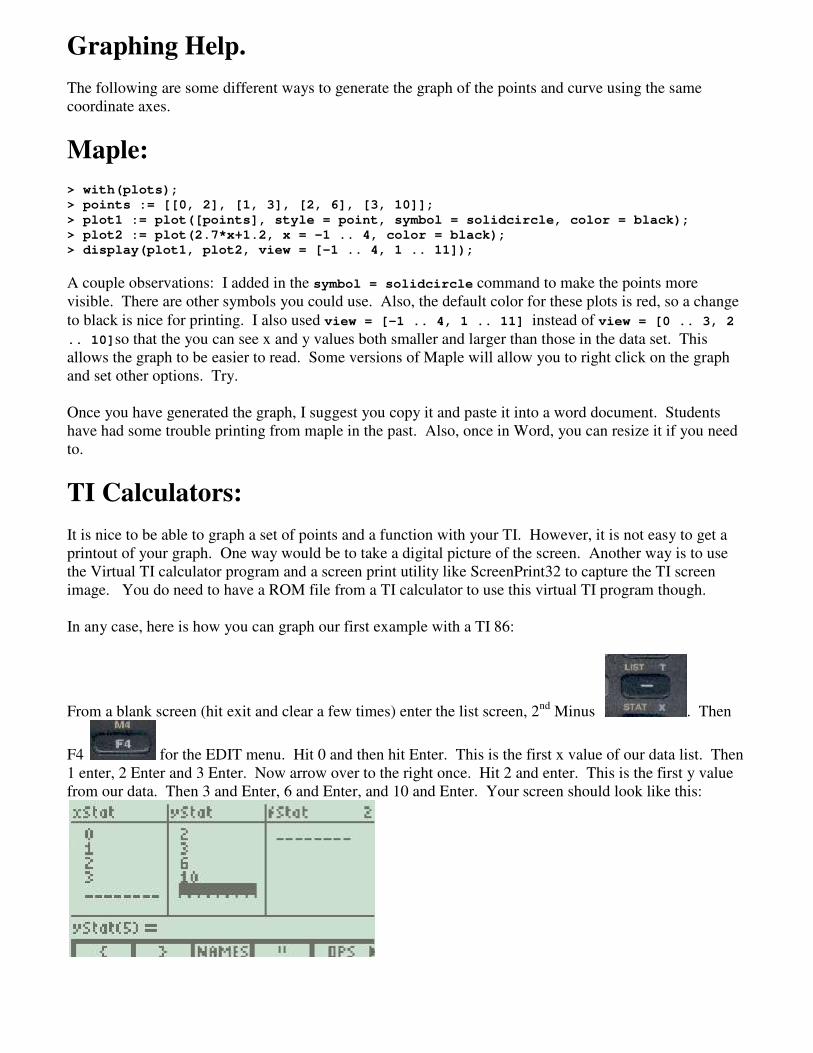
Graphing Help. The following are some different ways to generate the graph of the points and curve using the same coordinate axes.

Maple: > with(plots);

> points := [[0, 2], [1, 3], [2, 6], [3, 10]];

> plot1 := plot([points], style = point, symbol = solidcircle, color = black);

> plot2 := plot(2.7*x+1.2, x = -1 .. 4, color = black);

> display(plot1, plot2, view = [-1 .. 4, 1 .. 11]);

A couple observations: I added in the symbol = solidcircle command to make the points more visible. There are other symbols you could use. Also, the default color for these plots is red, so a change

to black is nice for printing. I also used view = [-1 .. 4, 1 .. 11] instead of view = [0 .. 3, 2

.. 10]so that the you can see x and y values both smaller and larger than those in the data set. This allows the graph to be easier to read. Some versions of Maple will allow you to right click on the graph and set other options. Try. Once you have generated the graph, I suggest you copy it and paste it into a word document. Students have had some trouble printing from maple in the past. Also, once in Word, you can resize it if you need to.

TI Calculators: It is nice to be able to graph a set of points and a function with your TI. However, it is not easy to get a printout of your graph. One way would be to take a digital picture of the screen. Another way is to use the Virtual TI calculator program and a screen print utility like ScreenPrint32 to capture the TI screen image. You do need to have a ROM file from a TI calculator to use this virtual TI program though. In any case, here is how you can graph our first example with a TI 86:

From a blank screen (hit exit and clear a few times) enter the list screen, 2nd Minus . Then

F4 for the EDIT menu. Hit 0 and then hit Enter. This is the first x value of our data list. Then 1 enter, 2 Enter and 3 Enter. Now arrow over to the right once. Hit 2 and enter. This is the first y value from our data. Then 3 and Enter, 6 and Enter, and 10 and Enter. Your screen should look like this:

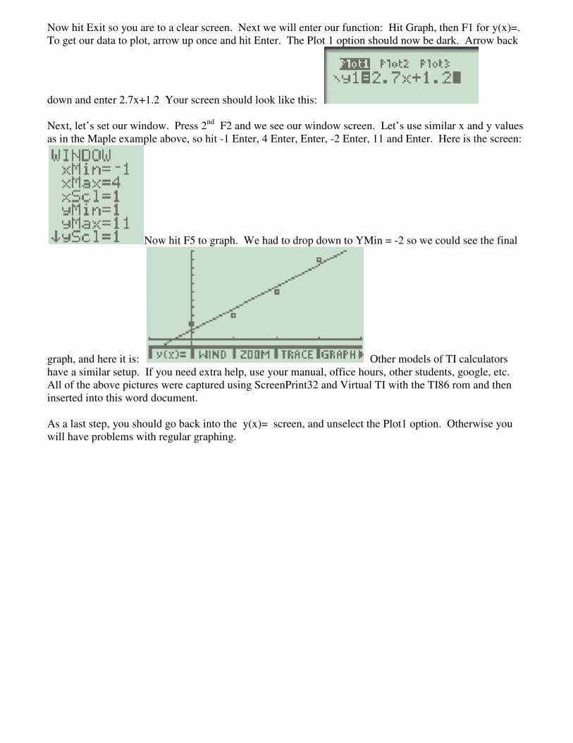
Now hit Exit so you are to a clear screen. Next we will enter our function: Hit Graph, then F1 for y(x)=. To get our data to plot, arrow up once and hit Enter. The Plot 1 option should now be dark. Arrow back

down and enter 2.7x+1.2 Your screen should look like this: Next, let’s set our window. Press 2nd F2 and we see our window screen. Let’s use similar x and y values as in the Maple example above, so hit -1 Enter, 4 Enter, Enter, -2 Enter, 11 and Enter. Here is the screen:

Now hit F5 to graph. We had to drop down to YMin = -2 so we could see the final

graph, and here it is: Other models of TI calculators have a similar setup. If you need extra help, use your manual, office hours, other students, google, etc. All of the above pictures were captured using ScreenPrint32 and Virtual TI with the TI86 rom and then inserted into this word document. As a last step, you should go back into the y(x)= screen, and unselect the Plot1 option. Otherwise you will have problems with regular graphing.

Excel:

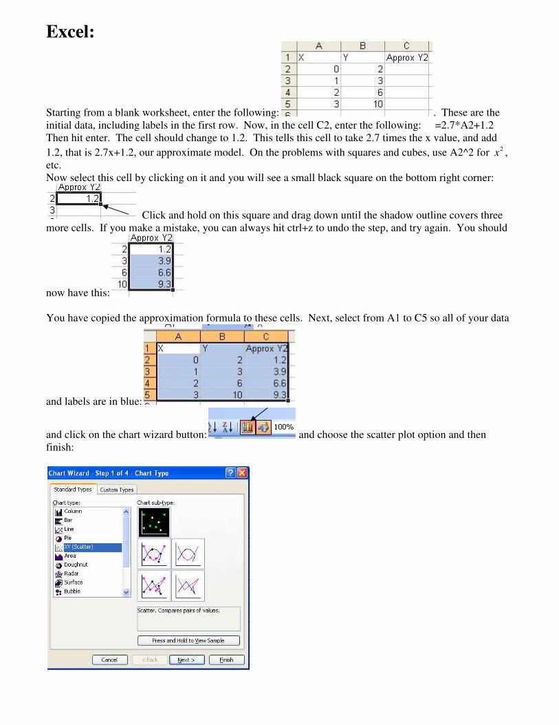
Starting from a blank worksheet, enter the following: . These are the initial data, including labels in the first row. Now, in the cell C2, enter the following: =2.7*A2+1.2 Then hit enter. The cell should change to 1.2. This tells this cell to take 2.7 times the x value, and add

1.2, that is 2.7x+1.2, our approximate model. On the problems with squares and cubes, use A2^2 for 2x ,

etc. Now select this cell by clicking on it and you will see a small black square on the bottom right corner:

Click and hold on this square and drag down until the shadow outline covers three more cells. If you make a mistake, you can always hit ctrl+z to undo the step, and try again. You should

now have this: You have copied the approximation formula to these cells. Next, select from A1 to C5 so all of your data

and labels are in blue:

and click on the chart wizard button: and choose the scatter plot option and then finish:

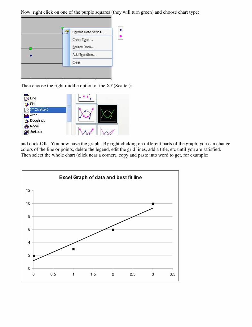
Now, right click on one of the purple squares (they will turn green) and choose chart type:

Then choose the right middle option of the XY(Scatter):

and click OK. You now have the graph. By right clicking on different parts of the graph, you can change colors of the line or points, delete the legend, edit the grid lines, add a title, etc until you are satisfied. Then select the whole chart (click near a corner), copy and paste into word to get, for example:

Excel Graph of data and best fit line

0

2

4

6

8

10

12

0 0.5 1 1.5 2 2.5 3 3.5

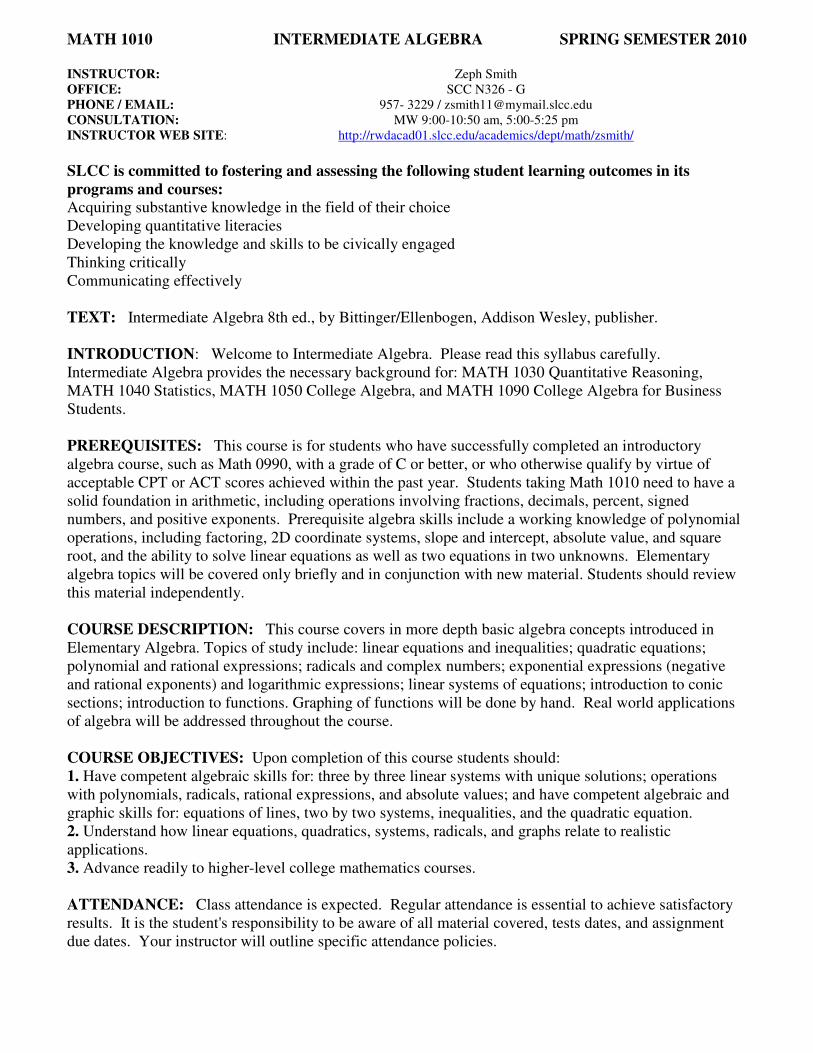
MATH 1010 INTERMEDIATE ALGEBRA SPRING SEMESTER 2010 INSTRUCTOR: Zeph Smith OFFICE: SCC N326 - G

PHONE / EMAIL: 957- 3229 / zsmith11@mymail.slcc.edu CONSULTATION: MW 9:00-10:50 am, 5:00-5:25 pm INSTRUCTOR WEB SITE: http://rwdacad01.slcc.edu/academics/dept/math/zsmith/

SLCC is committed to fostering and assessing the following student learning outcomes in its

programs and courses:

Acquiring substantive knowledge in the field of their choice Developing quantitative literacies Developing the knowledge and skills to be civically engaged Thinking critically Communicating effectively TEXT: Intermediate Algebra 8th ed., by Bittinger/Ellenbogen, Addison Wesley, publisher. INTRODUCTION: Welcome to Intermediate Algebra. Please read this syllabus carefully. Intermediate Algebra provides the necessary background for: MATH 1030 Quantitative Reasoning, MATH 1040 Statistics, MATH 1050 College Algebra, and MATH 1090 College Algebra for Business Students. PREREQUISITES: This course is for students who have successfully completed an introductory algebra course, such as Math 0990, with a grade of C or better, or who otherwise qualify by virtue of acceptable CPT or ACT scores achieved within the past year. Students taking Math 1010 need to have a solid foundation in arithmetic, including operations involving fractions, decimals, percent, signed numbers, and positive exponents. Prerequisite algebra skills include a working knowledge of polynomial operations, including factoring, 2D coordinate systems, slope and intercept, absolute value, and square root, and the ability to solve linear equations as well as two equations in two unknowns. Elementary algebra topics will be covered only briefly and in conjunction with new material. Students should review this material independently. COURSE DESCRIPTION: This course covers in more depth basic algebra concepts introduced in Elementary Algebra. Topics of study include: linear equations and inequalities; quadratic equations; polynomial and rational expressions; radicals and complex numbers; exponential expressions (negative and rational exponents) and logarithmic expressions; linear systems of equations; introduction to conic sections; introduction to functions. Graphing of functions will be done by hand. Real world applications of algebra will be addressed throughout the course. COURSE OBJECTIVES: Upon completion of this course students should: 1. Have competent algebraic skills for: three by three linear systems with unique solutions; operations with polynomials, radicals, rational expressions, and absolute values; and have competent algebraic and graphic skills for: equations of lines, two by two systems, inequalities, and the quadratic equation. 2. Understand how linear equations, quadratics, systems, radicals, and graphs relate to realistic applications. 3. Advance readily to higher-level college mathematics courses. ATTENDANCE: Class attendance is expected. Regular attendance is essential to achieve satisfactory results. It is the student's responsibility to be aware of all material covered, tests dates, and assignment due dates. Your instructor will outline specific attendance policies.

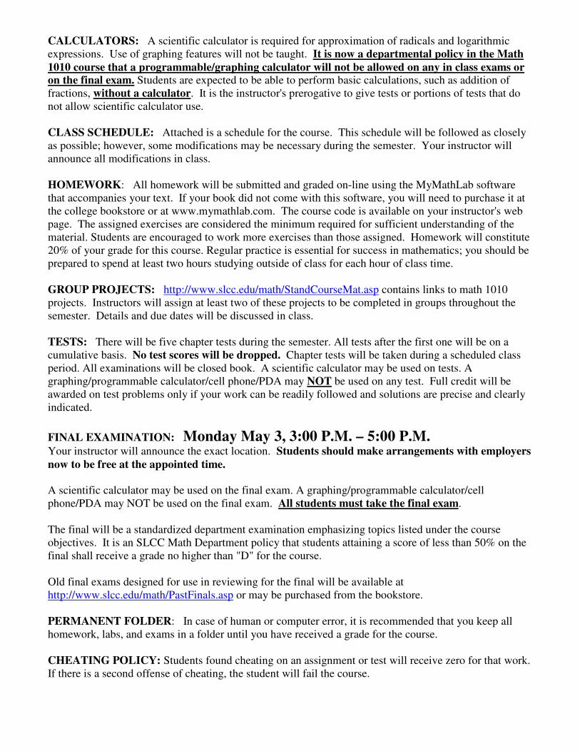
CALCULATORS: A scientific calculator is required for approximation of radicals and logarithmic expressions. Use of graphing features will not be taught. It is now a departmental policy in the Math

1010 course that a programmable/graphing calculator will not be allowed on any in class exams or

on the final exam. Students are expected to be able to perform basic calculations, such as addition of fractions, without a calculator. It is the instructor's prerogative to give tests or portions of tests that do not allow scientific calculator use.

CLASS SCHEDULE: Attached is a schedule for the course. This schedule will be followed as closely as possible; however, some modifications may be necessary during the semester. Your instructor will announce all modifications in class. HOMEWORK: All homework will be submitted and graded on-line using the MyMathLab software that accompanies your text. If your book did not come with this software, you will need to purchase it at the college bookstore or at www.mymathlab.com. The course code is available on your instructor's web page. The assigned exercises are considered the minimum required for sufficient understanding of the material. Students are encouraged to work more exercises than those assigned. Homework will constitute 20% of your grade for this course. Regular practice is essential for success in mathematics; you should be prepared to spend at least two hours studying outside of class for each hour of class time. GROUP PROJECTS: http://www.slcc.edu/math/StandCourseMat.asp contains links to math 1010 projects. Instructors will assign at least two of these projects to be completed in groups throughout the semester. Details and due dates will be discussed in class. TESTS: There will be five chapter tests during the semester. All tests after the first one will be on a cumulative basis. No test scores will be dropped. Chapter tests will be taken during a scheduled class period. All examinations will be closed book. A scientific calculator may be used on tests. A graphing/programmable calculator/cell phone/PDA may NOT be used on any test. Full credit will be awarded on test problems only if your work can be readily followed and solutions are precise and clearly indicated.

FINAL EXAMINATION: Monday May 3, 3:00 P.M. – 5:00 P.M. Your instructor will announce the exact location. Students should make arrangements with employers

now to be free at the appointed time. A scientific calculator may be used on the final exam. A graphing/programmable calculator/cell phone/PDA may NOT be used on the final exam. All students must take the final exam. The final will be a standardized department examination emphasizing topics listed under the course objectives. It is an SLCC Math Department policy that students attaining a score of less than 50% on the final shall receive a grade no higher than "D" for the course. Old final exams designed for use in reviewing for the final will be available at http://www.slcc.edu/math/PastFinals.asp or may be purchased from the bookstore. PERMANENT FOLDER: In case of human or computer error, it is recommended that you keep all homework, labs, and exams in a folder until you have received a grade for the course.

CHEATING POLICY: Students found cheating on an assignment or test will receive zero for that work. If there is a second offense of cheating, the student will fail the course.

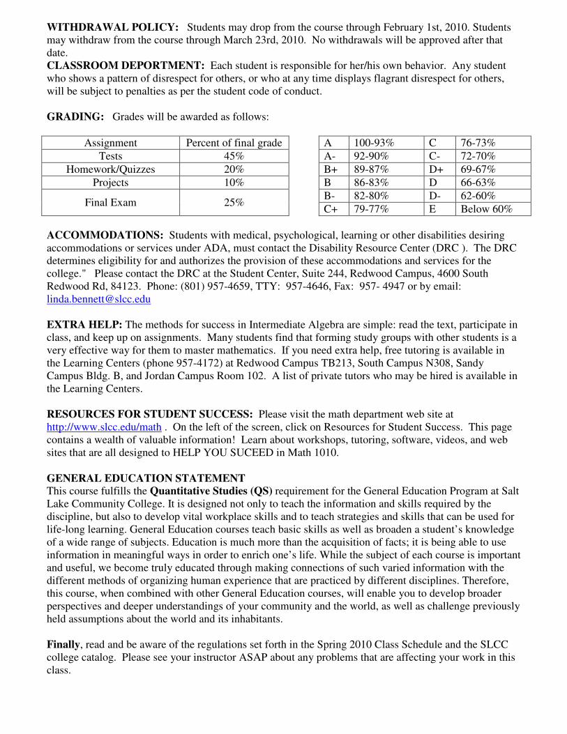
WITHDRAWAL POLICY: Students may drop from the course through February 1st, 2010. Students may withdraw from the course through March 23rd, 2010. No withdrawals will be approved after that date. CLASSROOM DEPORTMENT: Each student is responsible for her/his own behavior. Any student who shows a pattern of disrespect for others, or who at any time displays flagrant disrespect for others, will be subject to penalties as per the student code of conduct.

GRADING: Grades will be awarded as follows:

Assignment Percent of final grade A 100-93% C 76-73%

Tests 45% A- 92-90% C- 72-70%

Homework/Quizzes 20% B+ 89-87% D+ 69-67%

Projects 10% B 86-83% D 66-63%

Final Exam 25% B- 82-80% D- 62-60%

C+ 79-77% E Below 60%

ACCOMMODATIONS: Students with medical, psychological, learning or other disabilities desiring accommodations or services under ADA, must contact the Disability Resource Center (DRC ). The DRC determines eligibility for and authorizes the provision of these accommodations and services for the college." Please contact the DRC at the Student Center, Suite 244, Redwood Campus, 4600 South Redwood Rd, 84123. Phone: (801) 957-4659, TTY: 957-4646, Fax: 957- 4947 or by email: linda.bennett@slcc.edu EXTRA HELP: The methods for success in Intermediate Algebra are simple: read the text, participate in class, and keep up on assignments. Many students find that forming study groups with other students is a very effective way for them to master mathematics. If you need extra help, free tutoring is available in the Learning Centers (phone 957-4172) at Redwood Campus TB213, South Campus N308, Sandy Campus Bldg. B, and Jordan Campus Room 102. A list of private tutors who may be hired is available in the Learning Centers. RESOURCES FOR STUDENT SUCCESS: Please visit the math department web site at http://www.slcc.edu/math . On the left of the screen, click on Resources for Student Success. This page contains a wealth of valuable information! Learn about workshops, tutoring, software, videos, and web sites that are all designed to HELP YOU SUCEED in Math 1010.

GENERAL EDUCATION STATEMENT

This course fulfills the Quantitative Studies (QS) requirement for the General Education Program at Salt Lake Community College. It is designed not only to teach the information and skills required by the discipline, but also to develop vital workplace skills and to teach strategies and skills that can be used for life-long learning. General Education courses teach basic skills as well as broaden a student’s knowledge of a wide range of subjects. Education is much more than the acquisition of facts; it is being able to use information in meaningful ways in order to enrich one’s life. While the subject of each course is important and useful, we become truly educated through making connections of such varied information with the different methods of organizing human experience that are practiced by different disciplines. Therefore, this course, when combined with other General Education courses, will enable you to develop broader perspectives and deeper understandings of your community and the world, as well as challenge previously held assumptions about the world and its inhabitants. Finally, read and be aware of the regulations set forth in the Spring 2010 Class Schedule and the SLCC college catalog. Please see your instructor ASAP about any problems that are affecting your work in this class.