44
Douglas Laxton Economic Modeling Division January 30, 2014

Douglas Laxton
Economic Modeling Division January 30, 2014

The GPM Team Produces quarterly projections before each WEO
WEO numbers are produced by the country experts in the area departments
Models used to help impose macro consistency in the WEO (United States, Euro Area, Japan, Emerging Asia, Latin America and Remaining Countries)
Models used to produce risk assessments
Produces monthly updates for GDP growth 1 year ahead
Produces weekly note on recent economic developments

Key Models used for Production The Global Integrated Monetary and Fiscal Model
(GIMF)
The Global Economy Model (GEM)
The Global Projection Model (GPM)
The Flexible System of Global Models (FSGM) comprised of three modules (G20MOD, EUROMOD, EMERGMOD)

The Global Projection Model (GPM)
GPM is primarily a forecasting model whereas GIMF, GEM and FSGM are used for scenarios and policy analysis
GPM is the simplest model in terms of structure
It is a reduced-form model with only a handful of key behavioral equations
Smaller size makes system estimation of model parameters feasible
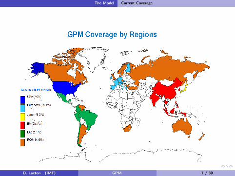
The main production version contains six regions: the United States, the euro area, Japan, Emerging Asia, Latin America, and the rest of the world

The Global Projection Model (GPM)
Several other versions of GPM have been developed
A euro area version has been built for the European Department which models individually Germany, France, Italy and Spain
A seven region version has been built that includes China individually.
An eleven region one is being developed that includes more individual Asian economies

The Global Projection Model : An Overview
Douglas Laxton and GPM team
Economic Modeling Division, Research Department, IMF
GPM Network Meeting, Paris, FranceJuly 1, 2013
D. Laxton (IMF) GPM July 1, 2013 1 / 39
Outline
Roadmap
Background and Motivation
Stages in model building
Structure of the model
Confronting model with data
Applications
Ongoing Work
D. Laxton (IMF) GPM July 1, 2013 2 / 39

Motivation
Background and Motivation
Two types of models developed by the IMF in recent years and used incentral banks and by country desks
A small quarterly projection model (QPM) with 4 or 5 key equations(Berg, Karam, and Laxton)
DSGE models – usually based on stronger choice-theoreticfoundations
D. Laxton (IMF) GPM July 1, 2013 3 / 39

Motivation
Background and Motivation, cont.
To develop a series of country or regional small macro modelsincorporating real and financial linkages.
Use these models to assess global outlook and conduct risk scenarios
D. Laxton (IMF) GPM July 1, 2013 4 / 39

Motivation
GPM aims at providing consistent international forecasts
At present, projections of the external outlook at policymaking institutionsusually take the following approaches:
Use forecasts from commercial sources, including from think tanksand global banks
Use forecasts prepared by international organizations
Build internal models
Potential problems with these approaches
Consistency
Timing and frequency of forecast updates
Resource constraints to develop macro models
How to implement risk analysis
D. Laxton (IMF) GPM July 1, 2013 5 / 39
Stages in model building
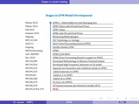
Winter2012 GPM11‐GlobalSpilloversandEmergingAsiaWinter2012 GPM7‐ChinawithOilandFoodPricesFall2012 GPM7‐ChinaSummer2012 GPM6withOilandFoodPricesOngoing MonitoringMethodologiesWP/12/109 Oil:Technologyvs.Geology2010‐11 ShortTermForecastingSystem(STFS)Ongoing SatelliteModelsGPM+WP/Forthcoming GPM6
StagesinGPMModelDevelopment
G20_REPORT GPM6(G20‐MAP)Dec.2010 GPM6(FirstForecastingRoundinsupporttoWEO)WP/10/285 DevelopedMethodologytoMeasurePotentialOutputWP/10/256 DevelopedHighFrequencyIndicatorstoUSmodelWP/09/214 Imposednon‐linearitiesandconfidencebandstoGPM3WP/09/255 AddedIndonesiatoGPM3WP/09/85 AddedL.A.toGPM3WP/08/280 AddedoiltoGPM3WP/08/279 US,Euro,JA(GPM3)WP/08/278 US(closedeconomyplusfinancialvariable,BLT)WP/05/278&279 FPAS
D. Laxton (IMF) GPM July 1, 2013 6 / 39
The Model Current Coverage
D. Laxton (IMF) GPM July 1, 2013 7 / 39

The Model Stochastic Processes
GPM shocks
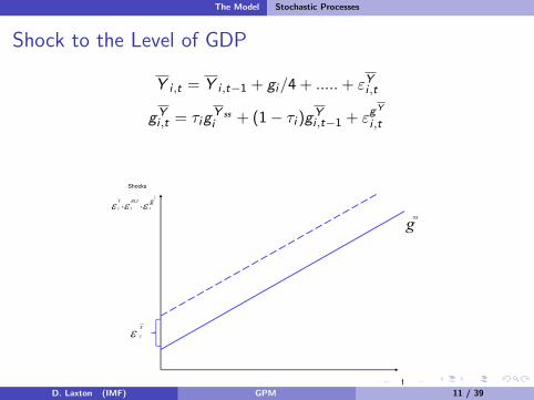
GPM allows for various shocks to explain unanticipated movements inthe data and to account for revisions in the underlying forecast. ForGDP, these revisions can result in transitory changes, temporary butpersistent changes, permanent changes and persistent changes in thegrowth rate
Examples of simple stochastic process to explain forecasts revisions topotential output and the NAIRU.
D. Laxton (IMF) GPM July 1, 2013 8 / 39

The Model Stochastic Processes
Potential Output
Y i ,t = Y i ,t−1 + gi/4− σ1,idotRPOILwt + εYi ,t (1)
gYi ,t = τig
Y ssi + (1− τi )gY
i ,t−1 + εgY
i ,t (2)
NAIRU
U i ,t = U i ,t−1 + gUi ,t + εUi ,t (3)
gUi ,t = (1− αi ,3)gU
i ,t−1 + εgU
i ,t (4)
D. Laxton (IMF) GPM July 1, 2013 9 / 39

The Model Stochastic Processes
Real GDP in steady state
Y i ,t = Y i ,t−1 + gi/4 + .....+ εYi ,t
gYi ,t = τig
Y ssi + (1− τi )gY
i ,t−1 + εgY
i ,t
Shocks
Y
gY
t
BLT
t
Y
t ,,
gss
ttD. Laxton (IMF) GPM July 1, 2013 10 / 39
The Model Stochastic Processes
Shock to the Level of GDP
Y i ,t = Y i ,t−1 + gi/4 + .....+ εYi ,t
gYi ,t = τig
Y ssi + (1− τi )gY
i ,t−1 + εgY
i ,t
Shocks
Y
gY
t
BLT
t
Y
t ,,
gss
Y
t
ttD. Laxton (IMF) GPM July 1, 2013 11 / 39

The Model Stochastic Processes
Shock to the level and the growth rate of GDP
Y i ,t = Y i ,t−1 + gi/4 + .....+ εYi ,t
gYi ,t = τig
Y ssi + (1− τi )gY
i ,t−1 + εgY
i ,t
Shocks
Y
gY
t
BLT
t
Y
t ,,
gss
Y
t gY
t
ttD. Laxton (IMF) GPM July 1, 2013 12 / 39
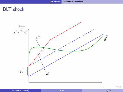
The Model Stochastic Processes
BLT shock
Shocks
Y
gY
t
BLT
t
Y
t ,,
gss BLT
t
Y
t gY
t
ttD. Laxton (IMF) GPM July 1, 2013 13 / 39

The Model Stochastic Processes
Stochastic processes for the real interest rate and the realexchange rate
Equilibrium real interest rate
RR i ,t = ρiRR i ,SS + (1− ρi )RR i ,t−1 + εRRi ,t (5)
Equilibrium real exchange rate
LZi ,t = 100 ∗ log(Si ,tPus,t/Pi ,t) (6)
∆LZi ,t = 100∆log(Si ,t)− (πi ,t − πus,t)/4 (7)
LZ i ,t = LZ i ,t−1 + εLZi ,t (8)
D. Laxton (IMF) GPM July 1, 2013 14 / 39
The Model Behavioral Equations
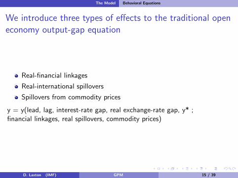
We introduce three types of effects to the traditional openeconomy output-gap equation
Real-financial linkages
Real-international spillovers
Spillovers from commodity prices
y = y(lead, lag, interest-rate gap, real exchange-rate gap, y* ;financial linkages, real spillovers, commodity prices)
D. Laxton (IMF) GPM July 1, 2013 15 / 39

The Model Behavioral Equations
Real-Financial linkagesThe model exploits information from the FED’s Senior-Loan officers survey.
Figure 2: U.S. Output Gap (Negative) and Lagged Bank Lending Tightening
1998 1999 2000 2001 2002 2003 2004 2005 2006 2007 2008 2009 20102
1
0
1
2
3
4
5
6
40
20
0
20
40
60
80
100
Output Gap BLT[t5]
(In percent)
D. Laxton (IMF) GPM July 1, 2013 16 / 39
The Model Behavioral Equations
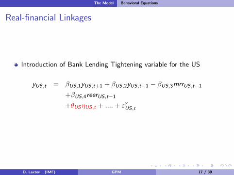
Real-financial Linkages
Introduction of Bank Lending Tightening variable for the US
yUS,t = βUS ,1yUS ,t+1 + βUS ,2yUS,t−1 − βUS,3mrrUS,t−1
+βUS ,4reerUS,t−1
+θUSηUS,t + ....+ εyUS ,t
D. Laxton (IMF) GPM July 1, 2013 17 / 39
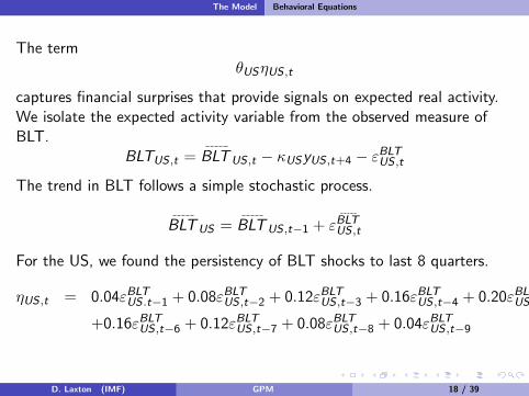
The Model Behavioral Equations
The termθUSηUS,t
captures financial surprises that provide signals on expected real activity.We isolate the expected activity variable from the observed measure ofBLT.
BLTUS ,t = BLTUS,t − κUSyUS,t+4 − εBLTUS,t
The trend in BLT follows a simple stochastic process.
BLTUS = BLTUS,t−1 + εBLTUS ,t
For the US, we found the persistency of BLT shocks to last 8 quarters.
ηUS ,t = 0.04εBLTUS .t−1 + 0.08εBLTUS,t−2 + 0.12εBLTUS ,t−3 + 0.16εBLTUS,t−4 + 0.20εBLTUS ,t−5
+0.16εBLTUS ,t−6 + 0.12εBLTUS,t−7 + 0.08εBLTUS ,t−8 + 0.04εBLTUS,t−9
D. Laxton (IMF) GPM July 1, 2013 18 / 39

The Model Behavioral Equations
Spillover Channels
Direct: foreign demand shocks∑j
ωi ,j ,5νj
Indirect: foreign output gaps, y*
Effect of commodity prices on income and wealth
βi ,6qi ,t
D. Laxton (IMF) GPM July 1, 2013 19 / 39

The Model Behavioral Equations
Output-Gap equation
yi ,t = βi ,1yi ,t+1 + βi ,2yi ,t−1 − βi ,3mrri ,t−1 (9)
+βi ,4reeri ,t−1 − {θiηi ,t}+∑j
ωi ,j ,5νj
+βi ,5∑j 6=i
ωi ,j ,5yj ,t−1
+βi ,6qi ,t + εyi ,t
D. Laxton (IMF) GPM July 1, 2013 20 / 39

The Model Behavioral Equations
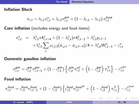
Inflation Block
Core inflation excludes food and energy prices. Model includes leads,lags, output gap, changes in exchange-rate gaps and past differencesbetween headline and core. The later term reflects the fact that foodand energy prices are inputs into the production process of othergoods and may also reflect the fact that workers may bargain on thebasis of headline inflation
Domestic gasoline prices depend on crude oil costs, taxes other factorinput costs as well as markups. The parameters are calibrated basedon available data on cost shares and the tax structure of each country.
Domestic food inflation: similar methodology as gasoline prices in thesense they are affected by international prices and other prices,”costs”.
D. Laxton (IMF) GPM July 1, 2013 21 / 39
The Model Behavioral Equations
Inflation Block
πi ,t = λi ,1πxi ,t + λi ,2π
gasi ,t + (1− λi ,1 − λi ,2)πfoodi ,t
Core inflation (excludes energy and food items)
πxi ,t = λxi ,1π4xi ,t+4 + (1− λxi ,1)π4xi ,t−1 + λxi ,2yi ,t−1
+λxi ,3∑j
ωi ,j ,3(zi ,j ,t − zi ,j ,t−4)/4 + λxi ,4W πi ,t−1 − επi ,t
Domestic gasoline inflation
πgasi ,t = ιgasi ,1 πgasi ,t−1 + (1− ιgasi ,1 )
{ιgasi ,2 π
oili ,t +
(1− ιgasi ,2
)πTi ,t
}− επgas
i ,t
Food inflation
πfoodi ,t = ιfoodi ,1 πfoodi ,t−1 + (1− ιfoodi ,1 ){ιfoodi ,2 πfood
W
i ,t +(
1− ιfoodi ,2
)πTi ,t
}− επfood
i ,t
D. Laxton (IMF) GPM July 1, 2013 22 / 39

The Model Behavioral Equations
Policy Interest Rate, inflation-forecast based rule
Ii ,t = γi ,1Ii ,t−1 +
(1− γi ,1){
RR i ,t + π4xi ,t+3 + γi ,2(π4xi ,t+3 − πtari
)+ γi ,4yi ,t
}+ εIi ,t
The termπ4xi ,t+3 = πxi ,t+3 + πxi ,t+2 + πxi ,t+1 + πxi ,t
is used because it allows monetary policy to react to current periodquarterly inflation rate
πxi ,t = 100 ∗ log(Pxi ,t/Px
i ,t−1)
in addition to forecasts of inflation
πxi ,t+1, πxi ,t+2, π
xi ,t+3
.
D. Laxton (IMF) GPM July 1, 2013 23 / 39

The Model Behavioral Equations
Uncovered Interest Rate Parity, risk-adjusted
(RRi ,t −RRus,t) = 4(LZ ei ,t+1 − LZi ,t) + (RR i ,t −RRus,t) + εRR−RRus
i ,t (10)
LZ ei ,t+1 = φi LZi ,t+1 + (1− φi ) LZi ,t−1 (11)
Unemployment Rate
ui ,t = αi ,1ui ,t−1 + αi ,2yi ,t + εui ,t (12)
D. Laxton (IMF) GPM July 1, 2013 24 / 39

The Model Behavioral Equations
World Commodity Prices
Oil and food prices are affected by global activity
For oil, we use a short-run price elasticity w.r.t. world income equal to9
For food, we use a short-run price elasticity w.r.t. world income equalto 0.8
Flexible process for the trends in prices. The oil price the trend isconsistent with recent empirical studies analyzing supply and demandconditions, see Benes and others (2013),
D. Laxton (IMF) GPM July 1, 2013 25 / 39

The Model Behavioral Equations
The block of commodity prices is defined as
Qwt = Q
wt + qw
t
Qwt = Q
wt−1 + gQ
w
t + εQw
t
gQw
t =(
1− ιQ3)
gQw
t−1 + εgQw
t
qwt = ιq1qw
t−1 + ιq2ywt + εq
w
t
For Q = {OIL,FOOD}, which denotes world’s oil and food real pricelevels, and q = {oil , food}, which denotes their cyclical component
D. Laxton (IMF) GPM July 1, 2013 26 / 39

Confronting model with data Bayesian Estimation
Advantages of Bayesian Methods
Puts some weight on priors and some weight on the data.
Incorporates theoretical insights to prevent incorrect empirical results,such as interest-rate movements having perverse effects on inflation,but also confronts model with the data to some extent.
Allows use of small samples without concern for incorrect estimatedresults.
Allows estimation of many coefficients and latent variables (e.g.,output gap, NAIRU, equilibrium real interest rate) even in smallsamples.
By specifying tightness of distribution on priors, researcher can changerelative weights on priors and data in determining posterior distribution forparameters.
D. Laxton (IMF) GPM July 1, 2013 27 / 39

Confronting model with data Parametrization in GPM
Full estimation is infeasible and we proceeded in stages:
Previous GPM work, particularly GPM6
Strong priors e.g., spillovers formulation, commodities block
D. Laxton (IMF) GPM July 1, 2013 28 / 39
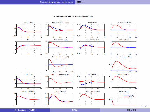
Confronting model with data IRFs
D. Laxton (IMF) GPM July 1, 2013 29 / 39

Confronting model with data IRFs
Cumulative 2 year Real GDP Growth Spillovers from a Demand Shock 1/Cumulative 2‐year Real GDP Growth Spillovers from a Demand Shock 1/‐Deviations from steady‐state, in percent‐
1/ Shock emitters in rows
D. Laxton (IMF) GPM July 1, 2013 30 / 39

Confronting model with data IRFs
Effect on the level of real GDP of a permanent 10% oil priceEffect on the level of real GDP of a permanent 10% oil price shock
‐Deviations from steady‐state, in percent‐
D. Laxton (IMF) GPM July 1, 2013 31 / 39

Confronting model with data IRFs
Effect on the level of real GDP of a transitory 10% oil price shock‐Deviations from steady‐state, in percent‐
D. Laxton (IMF) GPM July 1, 2013 32 / 39

Confronting model with data Forecasting Performance
RMSEs G3
D. Laxton (IMF) GPM July 1, 2013 33 / 39

Confronting model with data Forecasting Performance
RMSEs non‐G3
D. Laxton (IMF) GPM July 1, 2013 34 / 39
Applications
Construction of model-based global projections to help coordinate theWEO
Creation of risk scenarios for multilateral surveillance
Collaboration with Central Banks
D. Laxton (IMF) GPM July 1, 2013 35 / 39
Applications Construction of Model Based Forecast to the Global Economy
For WEO exercise, GPM-based forecast is a key ingredient
GPM-based forecast is augmented by near-term monitoring,conducted by GPM-team country experts at the IMF
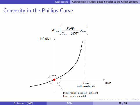
For simulation purposes, GPM considers two importantnon-linearities: zero interest floor and convex Phillips curve
D. Laxton (IMF) GPM July 1, 2013 36 / 39
Applications Construction of Model Based Forecast to the Global Economy
Convexity in the Phillips Curve
D. Laxton (IMF) GPM July 1, 2013 37 / 39
Applications Creation of Risk Scenarios
Since the model is non-linear, we have to conduct many draws ofsimulations to get estimates of the confidence bands
Probability of shocks being drawn corresponds to historical estimates
Monte Carlo simulation breaks because of the high dimensionality ofthe problem (number of shocks, number of periods and number ofstate variables)
D. Laxton (IMF) GPM July 1, 2013 38 / 39

Ongoing work
Ongoing work
Develop the next production version of the model (China)
D. Laxton (IMF) GPM July 1, 2013 39 / 39


