C C O O L L O O U U R R D D I I F F F F E E R R E E N N T T I I A A T T I I O O N N I I N N D D I I G G I I T T A A L L I I M M A A G G E E S S Zhenliang Shen This thesis is presented in fulfillment of the requirements for the degree of Master of Science School of Computer Science and Mathematics Victoria University of Technology Australia 2003
Transcript
CCOOLLOOUURR DDIIFFFFEERREENNTTIIAATTIIOONN
IINN DDIIGGIITTAALL IIMMAAGGEESS
Zhenliang Shen
This thesis is presented in fulfillment of the requirements
for the degree of Master of Science
School of Computer Science and Mathematics
Victoria University of Technology
Australia
2003
Declaration
Declaration
I declare that, to the best of my knowledge, this thesis contains no materials that have
been accepted for the award of any other degree or diploma in any university. It is
submitted in fulfillment of the candidature for the degree of Masters by Research at
Victoria University of Technology, Australia. The materials presented in this thesis are
the products of the author’s own independent research under the supervision of Dr.
Alasdair McAndrew.
Zhenliang Shen December 2003
i
Abstract
Abstract
To measure the quality of green vegetables in digital images, the colour appearance of the
vegetable is one of the main factors. In general, green colour represents good quality and
yellow colour represents poor quality empirically for green-vegetable. The colour
appearance is mainly determined by its hue, however, the value of brightness and
saturation affects the colour appearance under certain conditions. To measure the colour
difference between green and yellow, a series of experiments have been designed to
measure the colour difference under varying conditions. Five people were asked to
measure the colour differences in different experiments. First, colour differences are
measured as two of the values hue, brightness, and saturation are kept constant. Then, the
previous results are applied to measure the colour difference as one of the values hue,
brightness, and saturation is kept constant. Lastly, we develop a colour difference model
from the different values of hue, brightness, and saturation. Such a colour difference
model classifies the colours between green and yellow.
A windows application is designed to measure the quality of leafy vegetables by using
the colour difference model. The colours of such vegetables are classified to represent
different qualities. The measurement by computer analysis conforms to that produced by
human inspection.
ii
Acknowledgment
Acknowledgment
I am deeply indebted to my supervisor, Dr. Alasdair McAndrew, for his patient,
encouraging supervision, invaluable guidance and assistance, and constructive criticism
during the research and preparation of the thesis.
I gratefully acknowledge Dr. Hao Shi, for her introduction of this project and her
enlightening advice and suggestion. Also, I appreciate Mr. Graeme Thomson, sponsor of
Institute of Horticultural Development, Agriculture Victoria, for his supporting of this
project.
iii
Table of contents
Table of Contents
Declaration………………………………………………………………………...……..i
Abstract……………………………………………………………………………. …….ii
Acknowledgment………………………………………………………………….. ……iii
Table of Contents…………………………………………………………………. ……iv
List of Figures……………………………………………………………………... …..viii
List of Tables……………….……………………………………………...............……..x
1. Introduction ………………………………………………………………. ……..1
2. Research Background ……. .…….. ……..……………………………….……..3
2.1 Introduction… ……………………………………………………………..3
2.2 The Properties of Light..........…..…………………………………………4
2.3 Colour Fundamentals.……………………………………………………..6
2.3.1 Stimuli of Human Eyes…………………………………….. ……..7
2.3.2 Tri-chromatic Theory………………………………………. ……..8
2.3.3 The CIE Chromaticity System……………………………... ……..9
2.3.4 Colour Gamut ……...…………………………………………….11
2.4 Colour Model ...………………………………………………………….11
2.4.1 RGB Colour Model… ……………………………………………12
2.4.2 CMY Colour Model………………………………………...……13
2.4.3 YIQ Colour Model…………………………………………. ……14
iv
Table of contents
2.4.4 HSV Colour Model...….…………………………………… ……14
2.4.5 CIEL*a*b* Colour Model ………………………………… ……16
2.5 Colour Difference and Colour Tolerance…………………………. ……17
2.6 Just Noticeable Differences..…………...……………… ...… ...………..19
2.7 Summary…………………………………………………………… ……20
3. Colour Displaying and Measurement…………………………………... ……21
Table 3-4 Colour values in different colour models
28
Chapter 3 - Colour displaying and measurement
3.5.2 HSV colour measurement The HSV colour model uses three primary values, based on human perception, to
represent the colour. Colour 1 in table 3-4 is represented that it has the maximum values
of intensity and saturation and its hue is presented at 240 degree in a circle hue panel,
which is blue. As we have seen in figure 2-9, the hue value in HSV is defined from 0 to 1,
which may be considered as the ratio from 0 to 360 degree in a circle. Colours 2, 3, and 4
have the same hue value (0.333), but different saturation and brightness. Colour 3 is
darker than colour 2 and 4; and colour 4 is not a pure colour, as colours 2 and 3. HSV
colour model provides exactly same information as the RGB colour model but using
different description.
In the different colour model, the quantisation of acceptable different of colour is not
uniform. The advantage of the HSV colour model is not only to give more details for
general colours, but also to represent exactly the colour difference according to humans’
perception. The hue of colour 5 is 0.127, so this colour is located in the colour between
orange and yellow in the hue circle. Its brightness is 0.823; and its saturation is 0.60,
which means that this colour is plain compared with the pure colours. Colours 6 and 7 are
hard to distinguish their difference exactly using the RGB colour model. It is quite clear
to distinguish them in the HSV colour model. Since their hue values are 0.221 and 0.222
respectively, both colours have almost the same colour appearance in the visible
spectrum. Colour 6 is brighter than colour 7 because its intensity value is bigger than
colour 7. Although both colours are not pure, colour 7 is more colourful because its
saturation value is larger. In short, the HSV model gives a more useful description for
representing colours comparing with the RGB colour model; furthermore it has specified
values to definitely compare what the colour differences are. However, the values of
HSV have some disadvantages compared to human perception. Since the HSV colour
model is directly transformed from the RGB cube and its values are based on the RGB
values, in fact, its values correspond the changes of the CRT display rather than human
perception. The best colour model to describe colours according to human perception is
CIEL*a*b* (or CIELAB), which is based on the CIE XYZ model. [Fai98] [Fol96]
[For98]
29
Chapter 3 - Colour displaying and measurement
3.5.3 CIEL*a*b* colour measurement Colours 1 and 2 of table 3-4 have same brightness and saturation, only their hues differ,
being blue and green respectively. However, the human eye has different intensity
perception with different dominant wavelength. As the Figure 2-3 shows, green colours
normally appear brighter than blue colours with the same values of brightness and
saturation. According to the definition of CIEL*a*b*, L represents the brightness of the
colour. Therefore the brightness of colour 2 (Table 3-4) is much stronger than colour 1,
and this result is same as the human perception.
Figure 3-2 Colours of HSV with constant hue in CIEL*a*b*
The hue of CIEL*a*b* has the same definition as H in HSV. However, the hue of
CIEL*a*b* value is non-linear, which means CIE H value is not constant for the same
30
Chapter 3 - Colour displaying and measurement
dominant wavelength as the brightness and saturation varies. In Figure 3-2, twenty curves
are plotted with constant brightness, and hue and saturation varying for twenty different
colours. As the figure shows, each individual colour has the different hue values as the
saturation varies. This means that humans do not have the same hue perception for light
with the same frequency as the saturation is varying. In fact, the HSV colour model
represents the hue according to the physical properties of light, and the CIEL*a*b* or
CIEL*C*H* represents the hue varying acccording to human perception. [Bra98]
[Kue98] More the JND for green-yellow colour is referred in [Buc03] [Sut03].
3.6 Conclusion In conclusion, different colour models are used for different purposes. There is no single
colour model which can reproduce the colour and represent the colour differences
perfectly under all conditions. CIE XYZ is the foundation of colour science and
CIEL*a*b* is the best model to represent colour difference so far. Many advanced
colour models and formulae are based on CIEL*a*b*, such as CIEL*C*H*, CIE94,
CIECAM97s, and CIEDE2000. [Mel00]
31
Chapter 4 – Colour model conversions
Chapter 4
Colour model conversions
4.1 Introduction As we have discussed in the previous chapter, colour models are designed to reproduce
colours or differentiate colours for different purposes. Typically, there are two kinds of
colour models: device-dependent and device-independent. [Poynt] RGB and CMY are
typical device-dependent colour model because their colour reproduction are determined
by the output device. For example, the different phosphors of monitors and different inks
of printers require the use of colour models with different colour gamuts. Since IEC has
standardized the sRGB colour model used in CRT displays, any monitor using this
standard can be considered to be device-independent. Therefore, the values of different
colour models can be transformed to each other. [IEC98] [IEC99]
4.2 Conversion between RGB and HSV The HSV colour model can be considered as a different view of the RGB cube. Hence
the values of HSV can be considered as a transformation from RGB using geometric
methods. (See Figure 2-9) The diagonal of the RGB cube from black (the origin) to white
corresponds to the V axis of the hexcone in the HSV model. For any set of RGB values,
V is equal to the maximum value in this set. The HSV point corresponding to the set of
RGB values lies on the hexagonal cross section at value V. The parameter S is then
determined as the relative distance of this point from the V axis. The parameter H is
determined by calculating the relative position of the point within each sextant of the
32
Chapter 4 – Colour model conversions
hexagon. The values of RGB are defined in the range [0, 1], the same value range as
HSV. The value H is the ratio converted from 0 to 360 degree. The algorithm of the
conversion is as below: [Fol96] [Hea94]
Find the maximum and minimum values from the RGB triplet. The saturation, S,
is then:
maxmin)(max−
=S (4-1)
The Value, V, is
V = max (4-2)
The Hue, H, is calculated as follows. First calculate R’G’B’
minmax
max'−−
=RR
minmaxmax'
−−
=GG (4-3)
minmaxmax'
−−
=BB
If saturation, S, is zero then hue is undefined, which means that the colour has no
hue (it is a grey value), otherwise:
if R = max and G= min
H = 5 + B’ (4-4)
else if R = max and min≠G
H = 1 – G’ (4-5)
else if G = max and B = min
H = R’ + 1 (4-6)
else if G = max and min≠B
H = 3 – B’ (4-7)
else if R = min
H = 3 + G’ (4-8)
33
Chapter 4 – Colour model conversions
otherwise
H = 5 – R’ (4-9)
The numbers 1, 3, and 5 in the formulae from (4-4) to (4-9) are the ratios of degree of
360˚, for which 1 is equal to 60˚, 3 is equal to 180˚, and 5 is equal to 300˚. To convert
back from HSV to RGB is as below: [Fol96] [Hea94]
Firstly, there are some variables must be defined as follows:
The primary colour, which is the integer component of the value Hue
secondary colour = Hue – primary colour (4-10)
a = (1 – S) V (4-11)
b = (1 – (S * secondary colour)) V (4-12)
c = (1 – (S * (1 – secondary colour))) V (4-13)
Then, the RGB values can be calculated:
If primary colour = 0 then
R = V, G = c, B = a (4-14)
If primary colour = 1 then
R = b, G = V, B = a (4-15)
If primary colour = 2 then
R = a, G = V, B = c (4-16)
If primary colour = 3 then
R = a, G = b, B = V (4-17)
If primary colour = 4 then
R = c, G = a, B = V (4-18)
If primary colour = 5 then
R = V, G = a, B = b (4-19)
4.3 Conversion between RGB and CIE XYZ There are two RGB colour model values between image files and the phosphor dots of a
monitor. The digital image files store 8-bit linear RGB values and the phosphor dots of a
34
Chapter 4 – Colour model conversions
monitor represents non-linear sRGB value. There are two steps to convert RGB to CIE
XYZ values: [IEC98] [IEC99]
Step 1: Convert linear RGB value to non-linear sRGB value
0.255' 8 ÷= bitsRGB RR
0.255' 8 ÷= bitsRGB GG (4-20)
0.255' 8 ÷= bitsRGB BB
if ≤ 0.04045 sRGBR' , sRGBG' , sRGBB'
92.12' ÷= sRGBsRGB RR
92.12' ÷= sRGBsRGB GG (4-21)
92.12' ÷= sRGBsRGB BB
else if > 0.04045 sRGBR' , sRGBG' , sRGBB'
4.2
055.1055.0'
⎟⎠⎞
⎜⎝⎛ +
= sRGBsRGB
RR
4.2
055.1055.0'
⎟⎠⎞
⎜⎝⎛ +
= sRGBsRGB
GG (4-22)
4.2
055.1055.0'
⎟⎠⎞
⎜⎝⎛ +
= sRGBsRGB
BB
Step 2: Convert to CIE XYZ:
⎥⎥⎥⎥⎥
⎦
⎤
⎢⎢⎢⎢⎢
⎣
⎡
⎥⎥⎥⎥⎥
⎦
⎤
⎢⎢⎢⎢⎢
⎣
⎡
=
⎥⎥⎥⎥⎥
⎦
⎤
⎢⎢⎢⎢⎢
⎣
⎡
sRGB
sRGB
sRGB
D
B
G
R
Z
Y
X
9505.01192.00193.0
0722.07152.02126.0
1805.03576.04124.0
65
(4-23)
Converting CIE XYZ to RGB is as follows:
35
Chapter 4 – Colour model conversions
650570.12040.00557.0
0415.08758.19689.0
4986.05372.12406.3
DsRGB
sRGB
sRGB
Z
Y
X
B
G
R
⎥⎥⎥⎥⎥⎥
⎦
⎤
⎢⎢⎢⎢⎢⎢
⎣
⎡
⎥⎥⎥⎥⎥⎥
⎦
⎤
⎢⎢⎢⎢⎢⎢
⎣
⎡
−
−
−−
=
⎥⎥⎥⎥⎥⎥
⎦
⎤
⎢⎢⎢⎢⎢⎢
⎣
⎡
(4-24)
if , , ≤ 0.0031308 sRGBR sRGBG sRGBB
sRGBsRGB RR ×= 92.12'
sRGBsRGB GG ×= 92.12' (4-25)
sRGBsRGB BB ×= 92.12'
else if , , > 0.0031308 sRGBR sRGBG sRGBB
055.0055.1' )4.2/0.1( −×= sRGBsRGB RR
055.0055.1' )4.2/0.1( −×= sRGBsRGB GG (4-26)
055.0055.1' )4.2/0.1( −×= sRGBsRGB BB
The non-linear sR’G’B’ values are converted to digital code values which are determined
by two factors, WDC and KDC. Shown as below:
( ) KDCRKDCWDCR sRGBbit +×−= ')(8
( KDCGKDCWDCG sRGBbit )+×−= ')(8 (4-27)
( ) KDCBKDCWDCB sRGBbit +×−= ')(8
where WDC represents the white digital count and KDC represents the black digital count.
The IEC standard specifies a black digital count of 0 and a white digital count of 255 for
24-bit image encoding. So the resulting RGB values are:
sRGBbit RR '0.2558 ×=
sRGBbit GG '0.2558 ×= (4-28)
sRGBbit BB '0.2558 ×=
36
Chapter 4 – Colour model conversions
4.4 Conversions between CIE XYZ and CIEL*a*b* CIEL*a*b* is based directly on CIE XYZ (1931). It is non-linear and is intended to
mimic the logarithmic response of the human eye. The transformation is as below:
[Hof03]
⎪⎪⎪
⎩
⎪⎪⎪
⎨
⎧
≤⎟⎟⎠
⎞⎜⎜⎝
⎛×
>−⎟⎟⎠
⎞⎜⎜⎝
⎛×
=
008856.03.903
008856.016116
*
31
nn
nn
YYif
YY
YYif
YY
L (4-29)
⎟⎟⎠
⎞⎜⎜⎝
⎛⎟⎟⎠
⎞⎜⎜⎝
⎛−⎟⎟
⎠
⎞⎜⎜⎝
⎛×=
nn YYf
XXfa 500* (4-30)
⎟⎟⎠
⎞⎜⎜⎝
⎛⎟⎟⎠
⎞⎜⎜⎝
⎛−⎟⎟
⎠
⎞⎜⎜⎝
⎛×=
nn ZZf
YYfb 200* (4-31)
where
( )
⎪⎪
⎩
⎪⎪
⎨
⎧
≤+×
>
=
008856.011616787.7
008856.031
tift
tift
tf (4-32)
L* scales from 0 to 100 for relative luminance (Y / Yn) scaling 0 to 1.
Xn, Yn, and Zn are the values of reference white, which can be obtained from formula (4-
23). In the CRT displaying system, the white point is defined as 1 for the each primary
value. Therefore, Xn, Yn, and Zn can be obtained from formula 4-23 as:
⎥⎥⎥⎥⎥
⎦
⎤
⎢⎢⎢⎢⎢
⎣
⎡
⎥⎥⎥⎥⎥
⎦
⎤
⎢⎢⎢⎢⎢
⎣
⎡
=
⎥⎥⎥⎥⎥
⎦
⎤
⎢⎢⎢⎢⎢
⎣
⎡
1
1
1
9505.01192.00193.0
0722.07152.02126.0
1805.03576.04124.0
n
n
n
Z
Y
X
(4-33)
37
Chapter 4 – Colour model conversions
The CIEL*a*b* model converts to XYZ as the follows: [Hof03]
116
16*' +=
LY '500
*' YaX += '200
*' YbZ +−= (4-34)
( )
⎪⎪⎪
⎩
⎪⎪⎪
⎨
⎧
≤−
×
>×
=
206893.0'787.7
116/16'
206893.0'' 3
XifXX
XifXX
X
n
n
(4-35)
( )
⎪⎪⎪
⎩
⎪⎪⎪
⎨
⎧
≤−
×
>×
=
206893.0'787.7
116/16'
206893.0'' 3
YifYY
YifYY
Y
n
n
(4-36)
( )
⎪⎪⎪
⎩
⎪⎪⎪
⎨
⎧
≤−
×
>×
=
206893.0'787.7
116/16'
206893.0'' 3
ZifZZ
ZifZZ
Z
n
n
(4-37)
4.5 Conversions between CIEL*a*b* and CIEL*C*H* The conversion between CIEL*a*b* and CIEL*C*H* is a transformation between
Cartesian coordinates and polar coordinates. Polar parameters more closely match the
visual perception of colours. Their transformation is listed as below:
22 *** baC += (4-38)
⎟⎠⎞
⎜⎝⎛=
**arctan*
abH (4-39)
38
Chapter 4 – Colour model conversions
( ) **cos* CHa ×= (4-40)
( ) **sin* CHb ×= (4-41)
Figure 4-1 Three directions views of RGB in CIEL*a*b*
Different colour models can be converted to each other according to the above algorithms
and formulae. Since the colour gamut of RGB colour model is part of CIE XYZ, and
CIEL*a*b* has the same colour gamut as CIE XYZ, the transformation of RGB colour
can never fit within the CIEL*a*b* coordinate precisely. Figure 4-1 shows three
projections of the RGB gamut in the CIEL*a*b* coordinate system. The upper left
shows the relationship with the values L* and a*; the upper right figure shows the
coordinate with the values L* and b*; and the bottom figure represents the values in a*
and b* coordinate. Figure 4-2 shows four different three-dimensioned views. Hence, it is
clear that as the values are converted from the CIEL*a*b* colour model to the 24-bit
39
Chapter 4 – Colour model conversions
RGB colour model, some of the values are out of the RGB gamut and truncated to fit it.
Thus there could be errors when values are converted from CIEL*a*b* to RGB.
Figure 4-2 RGB colour gamut in CIEL*a*b* [Hof03]
4.6 CIE94 colour difference formula
CIE94 is a colour tolerance system rather than a colour model and it is based on the
value of CIEL*a*b*. Its formula is shown as below: [Gri02] [Luoro]
222
94***
⎟⎟⎠
⎞⎜⎜⎝
⎛ Δ+⎟⎟
⎠
⎞⎜⎜⎝
⎛ Δ+⎟⎟
⎠
⎞⎜⎜⎝
⎛ Δ=Δ
HH
ab
CC
ab
LL SKH
SKC
SKLE (4-42)
where
40
Chapter 4 – Colour model conversions
⎥⎥⎥
⎦
⎤
⎢⎢⎢
⎣
⎡
−−−
=⎥⎥⎥
⎦
⎤
⎢⎢⎢
⎣
⎡
ΔΔΔ
******
***
21
21
21
bbaaLL
baL
⎥⎥⎥
⎦
⎤
⎢⎢⎢
⎣
⎡
+
+=
⎥⎥⎥
⎦
⎤
⎢⎢⎢
⎣
⎡
22
22
21
21
2
1
**
**
*
*
ba
ba
C
C
*** 21 CCCab = ,
1=LS , *045.01 abC CS += , *015.01 abH CS +=
*** 21 CCCab −=Δ , 222 **** abab CbaH Δ−Δ+Δ=Δ
The CIE have defined reference conditions using this formula, that is: [Heggi]
1. The specimens are homogeneous in colour.
2. The colour difference (CIEL*a*b*) is <= 5 units.
3. They are placed in direct edge contact.
4. Each specimen subtends an angle of at least degrees to the assessor, whose
colour vision is normal.
5. They are illuminated at 1000 lux, and viewed against a background of uniform
grey, with L* of 50, under illumination simulating D65. (D65 is the light
source that is defined to simulate day-light and has x=0.312727 and
y=0.329024 in figure 2-6)
4.7 Conclusion The perception of colours is quite influenced by many external factors. It is
recommended to use a single colour model or colour difference formulae to reproduce or
measure colours. Some organizations, such as CIE, IEC, have released and standardized
some colour models and formulae to make the transformation among the different models
possible. However, no single colour model or colour difference formula is perfect so far.
Each model or formula just gives an approximate result compared with human perception.
Furthermore, nobody accepts or rejects colours because of numbers, it is the colour’s
appearance which counts. The final results must be confirmed by human visual
judgments. [Hof03] [Xri01] [Xri02]
41
Chapter 5 - Exploration of colour difference in MATLAB
Chapter 5
Exploration of colour difference in MATLAB
5.1 Introduction The aim of this chapter is the application of MATLAB to analyse colour differences in
digital images with the 24-bit RGB colour model, especially for the yellow-green colours,
which we have discussed in section 2.3 and 3.5.
MATLAB is very powerful for array operations. Since images are stored as two
dimensional arrays, images can be processed very quickly in MATLAB. Moreover, some
abstract data can be easily shown in a visual form using MATLAB. According to the
algorithms of colour conversion introduced in the last chapter, MATLAB can be used to
create images with different colours and using different colour models; these images will
be viewed by different people to distinguish the colour differences. The results are used
to analyse the relationship between human perception and the varying values in 24-bit
RGB colour model.
The RGB colour model as we have seen can be modeled as a cube. However, the
variation of its values does not conform to human perception. [Bro95] If all colours in 24-
bit RGB colour model are located in the CIEL*a*b* colour model with their
corresponding values, it is a quite irregular shape. (See Figure 4-1 and Figure 4-2) There
is no simple relationship between the 24-bit RGB colour model and the CIEL*a*b*
colour model and human perception as discussed in the last chapter. In this chapter,
42
Chapter 5 - Exploration of colour difference in MATLAB
several experiments are designed to analyse the relationship between human perception
and the variation of brightness, saturation, and hue. Ten people are asked to test the
colour difference in the each experiment. The maximum and minimum test values are
discarded in each experiment. The medium of other eight test results is used to analyse.
More details are listed in Appendix B and C. The three dimensions of the 24-bit RGB
colour model are decomposed to different layers in CIEL*a*b* colour model according
to the varying brightness, saturation, and hue value to show how the colours are
perceived with different parameters. Since the experiment is subjective test, there are
many factors to affect the results. In this thesis, all experiments are tested in the same
enviroment, for example, the same brightness and the same backgroud. The same monitor
is used for the all experiments and the voltage and the other conditions are all exactly
same. The motivation of the experiments is to use human perception to measure the
colour difference in RGB gamut.
5.2 Colours with same brightness of 24-bit RGB colour model in
CIEL*a*b* colour model
This experiment is designed to divide the CIEL*a*b* colour model into different layers
so that each layer has an identical value of brightness, and each layer only displays the
colours located in the 24- bit RGB model. The purpose of this experiment is to find how
the brightness affects the colour appearance.
In order to convert 24-bit RGB values to CIEL*a*b*, some new functions are created
with MATLAB:
Function rgb2lab converts RGB values to CIEL*a*b* values. The input 24-bit RGB
values can be either a single vector or a 3D array and the output CIEL*a*b* values have
the same type as input. Similarly, function lab2rgb converts CIEL*a*b* values to 24-bit
RGB values. The algorithm is shown in section 4.2, 4.3, and the MATLAB code is listed
in Appendix A. Since the CIEL*a*b* colour model is larger than the 24-bit RGB model,
as the values of CIEL*a*b* convert to 24-bit RGB values, some of them are out of the
range [0, 255]. In general, values less than 0 are considered as 0, and values more than
43
Chapter 5 - Exploration of colour difference in MATLAB
255 are considered as 255. Therefore, it is not always correct to use 24-bit RGB values to
represent the colours in CIEL*a*b* colour model. The MATLAB source codes are listed
in Appendix A.
The function lab2rgb_inrgbgamut is almost same as the function rgb2lab but only
colours are located in the 24-bit RGB colour model are converted; any colours out of the
24-bit RGB colour model are set to zero. The function lab2rgb_inrgbgamut thus can
display the relationship between 24-bit RGB and CIEL*a*b*. (The source codes are
listed in Appendix A) To show 24-bit RGB values in CIEL*a*b* colour model with the
same brightness, it can be done as below:
1. Create two 201 by 201 matrices to represent CIE a* and CIE b* values, because
the values of CIE a* and CIE b* are defined from –100 to +100. The CIE a*
matrix starts column 1 as value –100, the value of each next column is increased
by 1 from the current column, and end with column 201 as value 100. Each row
of the CIE a* matrix is exactly same. The CIE b* is created similarly as CIE a*,
which has the same value for each column, and the values of each row are
progressively increased by 1 from –100 to 100. (See below)
*10099099100
10099099100
10099099100
aCIE⎥⎥⎥⎥⎥⎥⎥
⎦
⎤
⎢⎢⎢⎢⎢⎢⎢
⎣
⎡
⋅⋅⋅⋅⋅⋅−−
⋅⋅⋅⋅⋅⋅⋅⋅⋅⋅⋅⋅⋅⋅⋅⋅⋅⋅⋅⋅
⋅⋅⋅⋅⋅⋅−−
⋅⋅⋅⋅⋅⋅−−
*100100100
999999
100100100
bCIE⎥⎥⎥⎥⎥⎥⎥⎥
⎦
⎤
⎢⎢⎢⎢⎢⎢⎢⎢
⎣
⎡
⋅⋅⋅⋅⋅
⋅⋅⋅⋅⋅⋅⋅⋅⋅⋅⋅⋅⋅⋅
−⋅⋅⋅⋅⋅⋅−−
−⋅⋅⋅⋅⋅⋅−−
Their values can be expressed:
100* , −= jCIEa ji (5-1)
100* , −= iCIEb ji (5-2)
where, matrix CIE a* and CIE b* have the exactly same size with the row and
column, i and j are varied in the same range [0, 200]
44
Chapter 5 - Exploration of colour difference in MATLAB
2. Create a matrix of the same size for the brightness values of CIEL*a*b*.
Elements of this matrix are constant with the constant in the range [0, 100]. Using
the function rgb_in_lab converts all these CIEL*a*b* values to RGB.
3. Since the output 24-bit RGB values are matrices which have the same size as the
input CIEL*a*b* values, each element of the matrices has the same coordinates
corresponding to the CIEL*a*b* colour model. The output 24-bit RGB values
can be considered as an image which presents one layer in CIEL*a*b* with the
specified brightness. In this image, all colours in the 24-bit RGB gamut are
displayed with their exact appearance, other colours out of the 24-bit RGB are set
to zero which appears black.
Function rgbinlab_brightness(arg1,arg2,arg3) can create different groups of colours of
24-bit RGB with same brightness in CIEL*a*b* colour model, using the same three
steps as above. The parameters arg1 and arg2 are the range of values of brightness, and
parameter arg3 is the step of the brightness varying in that range. The value of arg1 must
be less than arg2. If there is only one input parameter, only one image with that input
brightness value is created. By default, the step arg3 is initialized to value one. The
source code is listed in Appendix A. Figure 5-1 lists six images with different brightness.
(Appendix B lists more images with special values of brightness) As these images show,
colours are not uniformly distributed on each plane. At the low brightness for which the
value L* is less than 20 and the high brightness for which the value L* is more than 90,
the 24-bit RGB only has few colours in the CIEL*a*b* colour with the same brightness.
Furthermore, the blue colours appear mainly at low brightness values, and the yellow
colours are mainly located at high brightness value. Since this project is concerned with
measuring colours of green vegetables, the main purpose is to distinguish the colour
difference in the green and yellow areas. Five people were asked to distinguish the
colours with different brightness in these images: whether the colours are always same
with the same brightness but different hue and saturation. The results present that people
are not sensitive the colour difference as the colour is too dark or too bright (Table 5-1).
These results can be deduced from Table 5-1:
Result 1:
45
Chapter 5 - Exploration of colour difference in MATLAB
Any colour in 24-bit RGB colour model for which the value of brightness in
CIEL*a*b* is less than 10 can be considered as background because such a
colour cannot be perceived at the green and yellow parts, and the blue
colours do not appear in green vegetable.
Result 2:
Any colour in 24-bit RGB colour model for which the value of brightness in
CIEL*a*b* more than 95 appears as yellow or white.
46
Chapter 5 - Exploration of colour difference in MATLAB
Figure 5-1 Colours of 24-bit RGB in CIEL*a*b* with specific brightness
Person Level of brightness, at which
colours are too dark to distinguish
Level of brightness, at which
colours have no green appearance
1 12 93
2 10 94
3 12 95
4 10 93
5 12 94
Table 5-1 Results of measuring colours with different brightness
5.3 Colours with same hue of 24-bit RGB colour model in CIEL*a*b*
colour model The previous experiment showed how the colours are distributed at different brightness
levels. However, even with constant brightness, the number of colours is too great to
describe their details. The next experiment sets a constant hue value of CIEL*a*b* and
investigates the relationship between brightness and saturation. The perceived colour is
mainly determined by the value of hue. However, saturation and brightness also are very
important factors if the hue values are similar [Hun95]. In the next chapter, we shall
discuss the effects of brightness and saturation on colours with different hue values. Here,
47
Chapter 5 - Exploration of colour difference in MATLAB
all colours are supposed to have the same value of hue. As before, we shall conduct the
experiment using MATLAB routines:
Function rgbinlch_hue(arg1,arg2,arg3,arg4) converts all colours in 24-bit RGB colour
model with the same hue value to CIEL*C*H* colour model and displays the colours
according to the coordinate of CIEL*C*H*. This function is similar with the function
rgbinlab_brightness:
1. Create two 101 by 101 matrices to represent C* and L* value because the value
of C* and H* are varied in the range [0,100]. The values of matrices L* and C*
are similarly defined to the matrices CIE a* and CIE b* in the last experiment,
they can be expressed as the formulas below:
iL ji =,* (5-3)
jC ji =,* (5-4)
where, the values of i and j are varied in the range [0,100]. Every column of
matrix L* is same and the values of row are varied from 0 to 100; every row of
matrix C* is same and the values of column are varied from 0 to 100.
2. Create a 101 by 101 matrix with the same size as C* and L* to hold the hue
values. Hue values, H*, are constant comparing with the above C* and L*.
Changing the CIEL*C*H* values to CIEL*a*b* and then using the function
lab2rgb_inrgbgamut converts CIEL*a*b* values to 24-bit RGB values.
3. Display the output 24-bit RGB colours. All colours in the image have the same
hue values. The constant of the hue value can be chosen from 0 to 360 degree to
display more images as above for different hue values.
The parameter arg1 in the function rgbinlch_hue(arg1,arg2,arg3,arg4) is the size of the
output image. Since the numbers of row and column in the above matrices are same, the
output images are square and one parameter can describe their size. This value is same as
the numbers of pixels of the side in the image. Parameters arg2 and arg3 are the
minimum and maximum of the hue range. Parameter arg2 must be less than arg3.
Parameter arg4 is the step of the hue in its range. There are at least two and no more than
four input parameters in this function. If only two parameters are given, there is only one
output image, for which the hue value is defined by the second parameter. By default, the
48
Chapter 5 - Exploration of colour difference in MATLAB
hue step is one degree. The source code is listed in Appendix A. Figure 5-2 represents
colour appearance in the 24-bit RGB colour model for different brightness and saturation
and with a constant hue, H* set to 108 degree. This hue value has a yellow-green
appearance.
In figure 5-2, the brightness doesn’t affect the colour appearance very much. However, as
the saturation decreases to zero, this colour becomes paler. Five people were asked to
describe the colour difference with different saturation in this image and the result is
listed in table 5-2. We created five similar images, each with a constant hue value from 0
to 180 degrees (See Appendix B). Each image represents one major colour that is located
in the red, orange, yellow, and green areas of the CIEL*C*H* colour model. Five people
were asked to measure the colour difference of these images and the results are almost
the same as the result of Table 5-2.
49
Chapter 5 - Exploration of colour difference in MATLAB
Figure 5-2 Colours of RGB in CIEL*C*H* with 108 degree hue
We can conclude two further results:
Result 3:
If the colour is located in the red, yellow, and green area of the CIEL*C*H*
colour model, any colour in the 24-bit RGB colour model for which the value
of saturation in CIEL*C*H* is less than 10 can be considered as background
because such a colour is too pale to distinguish its colour appearance by
human perception.
Result 4:
If the colour is located in the red, yellow, and green area of the CIEL*C*H*
colour model, any colour in the 24-bit RGB colour model for which the value
of saturation in CIEL*C*H* is more than 80 can be considered as having the
same colour appearance because their colour differences are too small to
distinguish by human perception.
5.4 Colour difference with different value of hue The five images of the last experiment have their major hue appearance to represent red,
yellow, and green respectively. However, their hue differences are easy to distinguish.
The purpose of this experiment is designed to find the minimum hue difference that the
human eye can distinguish.
Person Maximum level of saturation at which
colours appear the same
Minimum level of saturation at
which colours appear the same
1 10 80
2 10 75
3 15 75
4 10 80
5 15 75
50
Chapter 5 - Exploration of colour difference in MATLAB
Table 5-2 Results of measuring colour with different hue
The MATLAB function rgbinlch_hue is used to create an image in which colours have the
same hue value, but different S, V. There are five groups of images created in this
experiment. Each group has nine images with one degree hue difference to the next one.
Their hue values are 42-50, 70-78, 100-108, 126-134, and 150-158 degrees respectively.
Figure 5-3 shows one group of images whose hue values are from 126-134. Ten people
were asked whether they can distinguish the colour difference in these nine images,
which are shown on the same monitor. (The hue values are not displayed on the images
and the orders of the images are random as these images were measured) The information
is collected and arranged in table 5-3:
51
Chapter 5 - Exploration of colour difference in MATLAB
Figure 5-3 Colours of 24-bit RGB in CIEL*C*H* with specific hue
The images are compared in irregular order, for example, hue 128 may be compared to
hue 129, 126, 134 or 130. The testing people do not know the hue value. Compared with
measuring the other groups of images, green and yellow colours have the same results.
Although the measurements of red colours are not same as the green and yellow colour
are distinguished their colour differences, they are not considered in this thesis because
we only focus the yellow and green colours.
The value of hue difference as two images are measured
Person Almost same Don’t know Different
1 Less than (including) 4 5 More than 5
2 Less than (including) 3 4 and 5 More than 5
3 Less than (including) 4 5 More than 6
4 Less than (including) 4 Nil More than 5
5 Less than (including) 3 4 More than 4
Table 5-3 Results of measuring hue difference Thus, a new result can be concluded from the table 5-3
Result 5:
For colours located in yellow and green areas of the CIEL*C*H* colour
model, if two such colours have the same values of brightness and saturation,
their colour appearance can be considered the same if their hue difference is
less than 4 degrees.
52
Chapter 5 - Exploration of colour difference in MATLAB
5.5 Colour difference with different saturation and brightness Humans as we have seen in section 3.5 like to describe colour differences using
brightness, hue, and saturation. [Hun96] In this project, as the quality of green vegetables
are measured, the greener the colour of the vegetable, the higher the quality the vegetable.
Yellow and orange colours usually indicate poor quality. So, it is most important to
measure the hue of the vegetable to determine its quality. To measure the hue degree of
two colours, it can be determined which colour is closer to orange, yellow, or green.
However, it is not yet clear how saturation and brightness affect human perception of the
vegetable. We will investigate this in the next chapter.
The next experiment investigates how people describe the colour difference if the colours
have same hue and brightness but different saturation, or the same hue and saturation but
different brightness. According to the five previous results, any colours whose saturation
is more than 80 and less than 10, or whose brightness is less than 10 do not need to be
considered. There are too many colours to measure. To make the experiment manageable,
five samples of hue are chosen to represent the main hue appearance which range over
the red, yellow, and green areas in the CIEL*C*H* colour model. Their values are 110,
120, 130, 140 and 150 degrees.
53
Chapter 5 - Exploration of colour difference in MATLAB
Figure 5-4 Colours of RGB in CIEL*C*H* with specific brightness and hue
5.5.1 Same hue and brightness with varying saturation In figure 5-2, colours do not only have varying saturation but also the varying brightness.
Therefore, colours with a given hue must be perceived with their saturation varying under
different brightness. The MATLAB function diffc_inlh is designed to create these kinds of
colours. The input parameters are the values of brightness and hue. The output images
have all colours with different saturation with the chosen values of brightness and hue
(for details, see the source code in Appendix A). In this experiment, four brightness
values are chosen to display the saturation varying in the each of the five sample hues,
their values are 30, 50, 70, and 90 respectively in the CIEL*C*H* colour model. Figure
5-4 is one of the examples for which the sample value is 130 degrees (more images are
listed in Appendix B). Five people were asked to view four such images to describe the
colour differences as the saturation varied. All answers indicate that the higher saturation
of the colour, the greener the colour; or the smaller saturation of the colour, the yellower
the colour (See the survey 1 of the Appendix C). Hence, a new result can be deduced
from this experiment:
Result 6:
54
Chapter 5 - Exploration of colour difference in MATLAB
If any colour has green and yellow appearance, and if their hue and
brightness value are constant, then the higher the saturation of this colour,
the greener this colour appears; inversely, the smaller the the saturation of
this colour, the yellower this colour appears.
As the saturation of the colour decreases, the colour gradually becomes pale and finally
becomes grey, which means no colour. Referring to our results 3, 4, and 6, we can deduce:
If two colours have similar hue value, and if their brightness values are same,
the higher the saturation they have, the more easily they can be distinguished.
5.5.2 Same hue and saturation with varying brightness The following experiment is similar to that discussed in the section 5.4.1. The MATLAB
function diffl_inch is designed to create these kinds of colours. The input parameters are
the values of saturation and hue. The output images have all colours with different
brightness for such saturation and hue (the source code is listed in Appendix A). The
same five sample hue values and four saturation values are chosen to measure the colour
difference with the varying brightness; the saturation values are 20, 35, 50, and 65 in the
CIEL*C*H* colour model. Figure 5-5 shows two sample images of this kind (others are
given in Appendix B). As five people were asked to view these images, there was the
same answer: the darker the colour is, the greener it looks with the same hue and
saturation values (see the survey 2 of the Appendix C). Here is the new result:
Result 7:
If the hue and saturation of colours are constant, the appearance of green
and green-yellow colours tends to a green hue as the brightness decreases
and to a yellow hue as the brightness increases.
55
Chapter 5 - Exploration of colour difference in MATLAB
Figure 5-5 Colours of RGB in CIEL*C*H* with specific brightness and saturation
5.6 Conclusion Using various colour properties, five experiments have been designed using MATLAB to
measure the colour difference with different conditions. Seven results have been obtained
from these experiments to measure colours in the CIEL*a*b* and CIEL*C*H* colour
models. These results conclude the general information of colour difference as the
brightness, hue, and saturation vary, and exclude some colours in the 24-bit RGB colour
model which are not available. It provides some simple methods for the further research
and provides in foundation for our next work. However, these results are obtained from a
particular condition: that is, that at least one of the brightness, hue, and saturation is
constant. Therefore, these results cannot be applied to general colour differences. In the
next chapter, colour differences will be analysed and discussed with all parameters
varying.
56
Chapter 6 – Development of colour difference in green vegetables
Chapter 6 Development of colour difference in green
vegetables
6.1 Introduction Freshness is an important factor in measuring the quality of the vegetables and freshness
is mainly determined by the colour appearance of the vegetable. For a green leafy
vegetable, such as broccoli, celery, and Chinese cabbages, the greener the colour of the
vegetable, the higher quality it has. Withered or rotten vegetables always have a yellow
or orange appearance. In this project, we only discuss how the colours indicate the quality
of vegetables. We shall show that the quality of green vegetables can be determined by
the number and appearance of green and yellow colours.
In the previous chapter, colour differences are explored according to their brightness, hue,
and saturation using MATLAB. Seven results were obtained from experiments. These
results provide general information of colour differences, especially for colours with red,
yellow, and green appearance. However, these results are only applicable under the
conditions that at least one of hue, saturation or brightness is constant. In this project,
colours are generated from images of leafy vegetables. Hence, colours must be measured
under more general conditions.
57
Chapter 6 – Development of colour difference in green vegetables
6.2 Colour difference in different conditions Normally, the appearance of a colour is mainly determined by its hue, for example green,
blue, or red. In the CIEL*C*H* colour model, the hue value increases as the colour
changes from yellow to green. Hence, the bigger the hue value of the colour, the greener
its appearance. Basically, yellow and green colours have the hue value between 70 to 150
degrees. According to result 5 in the chapter 5, colours appear the same if the hue
difference between them is less than 3 degrees; hence, only 28 hue levels can be
distinguished between green and yellow colours.
It is quite easy to check the colour difference by their hue difference. However, that
result is based on colours which have the same value of brightness and saturation.
According to other results in chapter 5, colour appearance is also determined by the
brightness and saturation. Therefore, hue measurement is not the only factor to affect the
colour appearance. If the hue difference is not evident, the brightness and saturation are
the main factors to affect the colour appearance. For example, if two colours (A and B)
have a green-yellow appearance, and if the hue value of colour A is five degrees greater
than the hue value of colour B, the colour A can be considered to have greener hue
appearance than colour B. However, if the saturation of the same colour A is much
smaller than colour B, colour A is paler than colour B. Does the pale colour A appear
greener than the vivid colour B?
The main purpose of this chapter is to investigate the colour appearance under all
possible conditions with green and yellow colours. To compare the colour difference
between two colours, there are seven possibilities to be checked for brightness, hue, and
saturation. Table 6-1 lists the all these possibilities. The colour differences in the
conditions 1, 2, and 3 have been analysed and discussed in chapter 5, where we have
obtained result 5 for condition 1, result 6 for condition 2, and result 7 for condition 3.
Condition 4 is obtained based on condition 2, and condition 5 is obtained based on
condition 3 to explore colour difference further. Condition 6 measures the colour
differences such as the colours in figure 5-2. Finally, in condition 7, colour differences
58
Chapter 6 – Development of colour difference in green vegetables
are explored and analysed in a real environment. The following experiments are designed
to measure the colour difference step by step under all these possible conditions.
Condition Brightness Hue Saturation
1 Same Different Same
2 Same Same Different
3 Different Same Same
4 Same Different Different
5 Different Different Same
6 Different Same Different
7 Different Different Different
Table 6-1 Colours varying with different condition
6.3 Minimum value of brightness and saturation difference by human
perception In chapter 5, the minimum value of hue difference by human perception with the same
brightness and saturation has been limited at three degrees. If the minimum values of
brightness and saturation difference by human perception also can be limited, then the
sample colours can be exactly chosen to measure their difference.
6.3.1 Minimum value of brightness difference with same hue and saturation To determine a minimum value of brightness difference, all possible colours with
different hue and saturation have to be considered. We will not analyse all possible
values of hue and saturation, but restrict our analysis to colours in the green and yellow
area in CIEL*C*H*, using a minimum hue difference of three degrees. In this
experiment, hue values are chosen from 70 to 150 degree with a 15 degree step giving six
hue values; saturation values are chosen from 20 to 80 in steps of 20. Since not all
colours in the CIEL*C*H* colour model are available in the RGB colour model (see
figure 4-2), not all values of brightness can be measured. There are 24 groups of colours
59
Chapter 6 – Development of colour difference in green vegetables
corresponding to the possible values of hue and saturation. We create the MATLAB
function sc_lch to produce the different colours. The input parameters of this function are
the three values of the CIEL*C*H* colour model. The output is an image with a single
colour of the input values (See the Appendix A for more details). Figure 6-1 lists some of
one group of colours for which the hue is 110 degree and the saturation is 70. In this case,
the values of brightness vary from 64 to 96. In this experiment, colours that have same
hue and saturation are set in the same group. Colours within the same group are
compared with each other only. As five people were asked to measure the colours from
these groups, most people were able to distinguish a difference of the colours even when
the colours have brightness difference by one or two. Hence we may conclude:
Figure 6-1 Colours with 110 degree hue and 70 saturation but different brightness
60
Chapter 6 – Development of colour difference in green vegetables
Result 8:
If colours have a green or yellow appearance, and if their values of hue and
saturation are constant, a brightness difference of one can be perceived.
Figure 6-2 Colours with 140 degree hue and 70 brightness but different saturation
6.3.2 Minimum value of saturation difference with same hue and brightness The measurement of the minimum saturation difference with the same hue and brightness
requires a similar experiment as the last one. Six hue values are chosen from 70 to 150
degree with a 15 degree step, and the values of brightness are chosen from 20 to 80 with
a step of 20. Also not all colours with all saturation values can be displayed in the RGB
61
Chapter 6 – Development of colour difference in green vegetables
colour model. The MATLAB sc_lch function is used to create these colours. Figure 6-2
lists some colours with different saturation for which the hue is 140 degrees and the
brightness is 70. Five people were asked to measure the colour difference from all groups,
nobody could distinguish the colour difference if the saturation difference is less than 4.
Here we may conclude:
Result 9:
If colours have a green or yellow appearance, and if their values of hue and
brightness are constant, their minimum perceivable saturation difference is 4.
According to result 8 and result 9, humans can distinguish colour difference with only 1
unit brightness difference and 4 units saturation difference. Therefore, in the
CIEL*C*H* colour mode, we may deduce that human eyes are more sensitive to
varying brightness than to varying saturation. [Fol96]
6.4 Colour measurement with different hue and saturation The purpose of this experiment is to find how the difference of both hue and saturation
simultaneously affect the appearance of colours with the same brightness. There are two
variables in this experiment, so it is more complicated than before. We create four groups
of colours with the brightness 40, 55, 70, and 85 respectively. In the RGB colour model,
as the value of brightness decreases, the maximum value of saturation also decreases,
especially for the green and yellow colours, because the RGB colour gamut is smaller
than that of CIEL*C*H* (See figure 5-2). If the brightness is chosen to be too small, the
range of saturation is too small to obtain a general result. According to the previous
results, the colour difference can be distinguished as the saturation varies within [10,80]
with the same hue and brightness, and the minimum saturation difference observable by
the human eye is 4. Therefore, we choose sample colour patches in this experiment
whose saturation varies from 10 to 82 with a step of 4 units. Figure 6-3 shows part of the
colour patches for which the hue values are varied from 110 to 129 degree with 1 degree
step. Since the minimum hue difference is 3 degrees and the minimum observable
saturation difference is 4 units, such colour patches almost cover enough colours for
sampling green-yellow colours with brightness of 70. There are four parts to this
experiment.
62
Chapter 6 – Development of colour difference in green vegetables
Figure 6-3 Colour patches of varying hue and saturation
with a fixed brightness value of 70
6.4.1 Minimum hue difference with different saturation
63
Chapter 6 – Development of colour difference in green vegetables
According to the result 5 in chapter 5, the minimum perceivable difference of hue with
colours of the same brightness and saturation is 3 degrees. Since the lower the saturation
of a colour, the paler it is, and pale colours are more difficult to distinguish than vivid
colours with the same brightness and hue (colours are too pale to distinguish their
appearance if the value of saturation is less than 10; see results 3 and 4); the minimum
perceivable hue difference depends on saturation. To check the minimum hue difference
under different saturation, colour patches with different hue and different saturation are
compared with each other. Table 6-2 has the result of the minimum hue differences with
different saturations after five people were asked to measure the colour patches in figure
6-3. According to the table 6-2, the minimum value of hue difference is rough linear
function of the saturation value. Based on result 5, we may conclude:
Minimum observable value of hue difference (degree)
Saturation Person 1 Person 2 Person 3 Person 4 Person 5
10 9 8 9 7 8
14 7 7 7 7 8
18 6 7 6 6 6
22 6 6 6 6 6
26 5 5 5 6 5
30 4 5 4 5 5
34 4 4 4 4 4
38 3 4 4 4 4
42 3 3 4 3 3
46 and more 3 3 3 3 3
Table 6-2 Minimum value of hue difference
Result 10:
If colours have a green or yellow appearance, and if the saturations of
colours are more than 42, their minimum perceivable hue difference is 3
degree at the same brightness and saturation; otherwise, as the saturation
64
Chapter 6 – Development of colour difference in green vegetables
decreases from 42 to 10, the minimum hue difference increases linearly from
3 to 8; and if the value of saturation is less than 10, colours can be considered
too pale to distinguish their hue difference.
6.4.2 Colour difference between more hue and saturation and less hue and
saturation
Since only the value of brightness is constant in this experiment, there are two different
conditions to be considered if there are two colours being measured: more hue with more
saturation comparing with less hue with less saturation; and more hue with less saturation
comparing with less hue with more saturation. According to the result 6 from the chapter
5, for colours with the same brightness and hue, the higher the saturation, the greener the
colours. Also, colours with higher hue tend to have greener appearance. Thus we
conclude that colours with higher saturation and hue value have a greener appearance
than colours with smaller saturation and hue value. For colours which are too similar to
be distinguished their difference by human perception, colours with more hue and
saturation are greener than the colours with less hue and saturation in theory. To prove
this result, six pairs of colours are created, and five people are asked to measure their
difference (See the table 6-3). The hue and saturation differences are chosen small
enough because large differences are easy to distinguish. Figure 6-4 lists such two pairs
of colours (The others are listed in the Appendix B). The results of measuring six pairs of
colours are exactly the same. The new result is:
Result 11:
If colours mainly have green or yellow appearance, and if the value of
brightness is constant, colours with large value of hue and saturation have
greener appearance than the small value of hue and saturation; conversely,
colours with small values of hue and saturation have yellower appearance
than colours with large values of hue and saturation.
Pair 1 Pair 2 Pair 3 Pair 4 Pair 5 Pair 6
65
Chapter 6 – Development of colour difference in green vegetables
L* 70 70 70 70 50 50 60 60 80 80 80 80
C* 65 70 65 70 40 44 55 60 70 74 50 54
H* 126 130 96 100 100 104 140 145 120 124 110 114
Table 6-3 Sample pairs of colours with specific values
Figure 6-4 Colours with more hue and saturation and less hue and saturation
6.4.3 Colour difference between colour with more hue with less saturation
and colours with less hue with more saturation This experiment is divided into four steps, which is shown in the following flow chart:
Step 1: Colour patches which have same hue in figure 6-3 are chosen as group A. Group
B has similar colour patches but their hue value is 3 degrees less than the colours in
group A. Each colour patch in group A is only compared with the colour patches of group
B having the bigger saturation value, in order to measure which colour is greener or
66
Chapter 6 – Development of colour difference in green vegetables
yellower. We created the MATLAB function dc_lch to produce two images with different
colours. The input parameters are two CIEL*C*H* values (See the Appendix A for
more details of the function. We mainly use this function to create two images with
different colours and measure their difference in this chapter). Five people were asked to
judge whether the colour patches with the less saturation in group B are greener than
colour patches with small saturation in group A. In this step, the values of hue are chosen
in the range from 70 to 150 (yellow and green appearance) and the brightness is constant
at 70. Table 6-4 lists parts of the different minimum values of saturation with 125 hue
value are greener than colour patches with 128 hue value.
Hue Saturation of colour patch with 125 hue is greener than 128 hue value
Person 128 10 14 18 22 26 30 34 38 42 46
1 125 14 18 26 34 38 46 58 66 82 -
2 125 14 18 26 34 42 46 58 70 78 -
3 125 14 22 26 30 42 50 62 70 82 -
4 125 14 18 36 34 42 50 54 70 82 -
5 125 18 22 26 34 42 54 62 74 82 -
Average 125 15 19 26 33 41 49 59 70 81 -
Table 6-4 Results of measuring threshold value of saturation
with 3 degree hue difference
According the results of table 6-4, the colour patches are too pale to distinguish if the
saturation is less than 10. If the saturation is more than 46, colour patches with hue of 128
are always greener than colour patches with hue of 125 for any value of saturation.
Therefore, if the saturation varies from 10 to 46, then colours with hue of 125 degree or
less, which have larger saturation value, have greener appearance than colours with hue
of 128 degrees.
67
Chapter 6 – Development of colour difference in green vegetables
Step 2: The hue difference (125 and 128 degrees) in the last step between two groups is 3
degrees. In this step, the colour patches of group A are same as last experiment have 128
hue degrees, but the colour patches of group B are instead of 122, 119 hue degrees. Again,
five people were asked to judge their colour difference. The results are listed in the table
6-5. The purpose of this step is to check whether colour difference varies linearly as the
values of hue and saturation vary.
Hue Saturation of colour patch with small hue is greener than 128 hue value
128 10 14 18 22 26 30 34 38 42 46 50 54
Average 125 15 19 26 33 41 49 59 70 81 - - -
Average 122 17 30 46 67 81 - - - - - - -
Average 119 24 49 75 - - - - - - - - -
Table 6-5 Average results of threshold value of saturation with different hue
Step 3: The value of group A in the previous steps was constant at 128. In this step, the
hue values of group A are chosen as 100, 115, and 145, for which such hue values have
the yellow and green appearance. The colours of group A with different hue values are
measured with the colours of group B with different hue values as in the above two steps.
Step 4: All values of brightness are 70 at the above three steps. In this step, the values of
brightness are chosen as 40, 55, and 85 to measure the colour difference using the same
methods as the above steps (The colour patches are created same as figure 6-3 with
different brightness, and the brightness of colour patches cannot be chosen too small
because the maximum value of saturation decreases as the brightness decreases in the
RGB colour model). The results are very similar as the table 6-5 as the brightness is
varied and the errors of each result are very tiny. Since colour perception is very
subjective, and even the person may measure colours differently, these errors can be
ignored (more results are listed in the survey 3 of Appendix C).
Each result for identical hue is very close to a straight line as the saturation value with
both small and big value. According to the standard linear regression function of
68
Chapter 6 – Development of colour difference in green vegetables
mathematical statistics, the result in table 6-4 can be found using the formula below:
[Hoe71]
)(' xxbyy −+= (6-1)
where, 2)(
)(
∑∑
−
−=
xxyxx
b , x is the value of saturation with more hue, y is the value of
saturation with small hue, x is the average value of x, and y is the average value of y.
The three results of table 6-4 can be expressed by the following equations:
4.101.2 128_125_ −×= HueHue SS (6-2)
262.4 128_122_ −×= HueHue SS (6-3)
425.6 128_119_ −×= HueHue SS (6-4)
Figure 6-5 Lines of equation 6-5 obtained from the values of experiments
69
Chapter 6 – Development of colour difference in green vegetables
Based on the equations 6-2, 6-3, and 6-4, the linear regression function is used again to
obtain an approximation to a linear result as the hue difference varies; the universal
equation can be expressed as below:
)5(72.0 __ −×Δ×= HueBigHueHueSmall SS (6-5)
where, is in the range of [10, 42], and HueBigS _ HueΔ is the hue difference between two
compared colours. Colours which have greater saturation than are greener than
the colours with saturation . The dots in figure 6-5 are the results of the
experiment for measuring colour patches, and the lines are drawn by using the equation
6-5 for the corresponding values of colours in MATLAB.
HueSmallS _
HueBigS _
In conclusion, the result is:
Result 12:
If the hue difference is more than 9 degrees, or if the saturation is more than 46,
colours with more hue value always are greener than less hue value colours. If the
hue difference is less than 9 degrees and the saturation is less than 46, then colours
with less hue and more saturation appear greener than colours with more hue and
less saturation. The varying of brightness and saturation is approximately linear,
their relation can be derived from the linear regression function of mathematical
statistics, and its general equation is listed in equation 6-5.
6.5 Colour measurements with different hue and brightness The effects of hue and saturation to colour appearance have been discussed in the last
section. However, we have based our investigation with brightness being constant.
According to result 8 and 9, the minimum brightness difference by human perception is
only one in one hundred units; the minimum saturation difference by human perception is
4 in one hundred units. Therefore humans are more sensitive to brightness than to
saturation. [Fol96] This experiment will explore and analyse how brightness affects the
appearance of colours with different hue, but with the same saturation. Similar colour
patches in the last experiment are created for people to measure, but this time the
70
Chapter 6 – Development of colour difference in green vegetables
saturation is constant. Since there are too many different colour patches, we won’t list all
the colour patches here. Figure 6-6 lists parts of the all sample colour patches, for which
the hue is from 120 to 138 with one degree step, brightness is from 30 to 94 with 2 step,
and the saturation is 50. The colour difference in the colour patches of figure 6-6 can be
classified into two types, which are more hue and brightness compared with less hue and
brightness, and more hue and less brightness compared with less hue and more brightness.
According to result 7 in chapter 5, a colour with less brightness has a greener appearance
than a colour with big brightness if the hue and saturation are same, and a colour with
more hue is greener than a colour with less hue if the brightness and saturation are same.
This can be stated as:
Result 13:
If colours mainly have green or yellow appearance, and if the value of
saturation is constant, colours with more hue and less brightness have
greener appearance than colours with less hue and big brightness; conversely,
colours with less hue and large brightness have yellower appearance than
colours with more hue and less brightness.
To measure colour differences between more hue and brightness and less hue and
brightness, a similar experiment is designed to measure the colour difference between
more hue and less saturation and less hue and more saturation. This experiment is divided
into four steps:
Step 1: A group colour patches ‘A’ of identical hue are compared with same group
colour patches ‘B’, but with two degree hue difference.
Step 2: The hue values of colours in the group ‘B’ are chosen to have 4, 6, 8, and 10
degree difference respectively, for comparing the colours in group ‘A’ as in step 1.
Step 3: The hue of first group is arbitrarily chosen from yellow to green; then the same
experiment is done as above.
Step 4: The previous three steps are repeated to measure the colour difference with
saturation other than 50.
71
Chapter 6 – Development of colour difference in green vegetables
Figure 6-6 Colour patches with different brightness and hue as the saturation is 50
Table 6-6 lists the results of the experiment as five people were asked to measure the
colour difference of colour patches in figure 6-6. The other results of colour difference
measurement in the step 3 and 4 are almost same (More results are listed in the survey 4
of Appendix C). As the table shows, as the hue difference increases, the brightness
decreases thus affecting the appearance of the hue. If the hue difference is more than 9,
the brightness only slightly affects the hue appearance. According to the linear regression
72
Chapter 6 – Development of colour difference in green vegetables
function 6-2, the three results with different hue of table 6-5 can be formulated as the
equation 6-6:
Hue Brightness of colour patch with small hue is greener than 138 hue value
(Saturation is 50)
138 90 86 82 78 74 70 66 62 58 54 50 46
Average 136 84 77 69 62 53 43 33 - - - - -
Average 134 76 63 51 - - - - - - - - -
Average 132 69 54 - - - - - - - - - -
Average 130 55
Table 6-6 Average testing results of threshold value of brightness with different hue
2)96( _
__HueBigHue
HueBigHueSmall
LLL
−×Δ−= (6-6)
where, is value of brightness at the range of [66, 90], and is the hue
difference between two compared colours. Since all results of this experiment are similar,
the equation 6-6 can be generally applied when the saturation is constant. The dots in
figure 6-5 are the results of the experiment for measuring colour patches with 2, 4, and 6
hue difference respectively, and the lines are drawn by using the equation 6-5 for the
corresponding values of colours in MATLAB. We can state this result:
HueBigL _ HueΔ
Result 14:
If the hue difference is more than 9 degrees, or if the brightness is less than 66,
colours with more hue value always appear greener than colours with less hue value,
independent of their brightness. If the hue difference is less than 9 degrees and the
brightness is more than 66, then some colours with less hue and brightness are
greener than colours with more hue and saturation. The brightness value of less hue
colours increases, as the brightness value of more hue colours increases; and it is
increasing as the hue difference increases. Equation 6-6 expresses the threshold
brightness values of colours with less hue compared with colours with more hue.
Colours which have smaller brightness value than the threshold value, , are
greener than the colour with .
HueSmallL _
HueBigL _
73
Chapter 6 – Development of colour difference in green vegetables
Figure 6-7 Lines of equation 6-6 obtained from the dots of experiment
6.6 Colour differences with varying brightness and saturation All previous experiments involve varying hue. According to those experiments, the hue is
the main factor in determining the colour appearance, but the brightness and saturation
also affects the colour appearance if the hue difference is slight. Normally, small
brightness or big saturation makes colours have greener appearance if the hue is constant;
conversely, big brightness or small saturation makes colours have yellower appearance.
Thus:
Result 15:
If colours have a green or yellow appearance, and if the value of hue is
constant, colours with big saturation and small brightness have greener
appearance than colours with small saturation and big brightness;
74
Chapter 6 – Development of colour difference in green vegetables
conversely, colours with small saturation and big brightness have yellower
appearance than colours with big saturation and small brightness.
There remains one condition to measure, in which a colour with big brightness and big
saturation is compared with a colour with small brightness and small saturation, with the
hue being constant. Figure 6-8 lists such colour patches of 125 degree hue as the
brightness and saturation have the four units steps each. There are four parts to this
experiment:
Figure 6-8 Colour patches with different brightness and saturation
as the hue is 125 degree
75
Chapter 6 – Development of colour difference in green vegetables
Step 1: Colour patches which have saturation of 88 but different brightness in figure 6-8
are chosen as sample colours. Colour patches whose saturation is 84 are compared to the
sample colours for determining their differences.
Step 2: Colours with different saturations which are 4, 8, 12, 16, and 20 units less
respectively are chosen for comparison with the sample colour patches.
Step 3: Repeat step 1 and step 2 but using different saturation of the sample colour
patches.
Step 4: Repeat parts 1, 2 and 3 for arbitrary hue of green and yellow.
Five people were asked to measure the colour difference of the colour patches. Table 6-7
lists the results of step 1 and step 2 using the colour patches shown in figure 6-8.
As table 6-7 shows, the values of brightness vary almost linearly as the saturation varies.
Comparing with other data of this experiment, they almost have the same results. This
result can be expressed by equations 6-7 and 6-8.
In conclusion, the results of this experiment can be represented as below:
S Brightness of colour patches with small S is greener than sample patches
Sample 88 88 84 80 76 72 68 64 60 56 52 48 44
Average 84 83 77 71 64 58 53 47 41 35 30 23 -
Average 80 77 70 63 58 52 47 41 36 30 24 -
Average 76 71 65 59 53 48 42 35 29 24 - -
Average 70 64 59 53 48 41 36 30 25 - - -
Average 63 58 52 45 39 34 29 22 - - - -
Table 6-7 Average results of threshold values of brightness with different saturation
Result 16:
If green or yellow colours have constant hue value, and conditions of result 13 do
not apply the brightness and saturation affect the colour appearance linearly. Their
relationship can be expressed by the equations 6-7 and 6-8. Equation 6-7 expresses
the minimum saturation for which colours with small brightness are greener than
76
Chapter 6 – Development of colour difference in green vegetables
colours with big brightness. Equation 6-4 provides the threshold ratio of saturation
difference and brightness difference between two colours to distinguish their hue
appearance; when the fraction of saturation and brightness is more than 2/3, the
colour with big saturation and big brightness is greener than the colour with small
saturation and small brightness. It is clear that the saturation is more sensitive than
brightness as for human measurement of hue appearance. (This does not contradict
with the result 8 and 9; since humans can distinguish a smaller difference of
brightness than saturation, but a small change of brightness doesn’t change the hue
appearance.)
BrightnessLBigLSmall SS Δ×−=32
__ (6-7)
32
=ΔΔ
Brightness
Saturation (6-8)
where, is the saturation difference of two colours, and SaturationΔ BrightnessΔ is the brightness
difference of two colours.
6.7 Colour difference under any condition So far, we have obtained 15 results from different experiments. Each result applies only
to some special condition, since each is obtained from the condition at least one of the
CIEL*C*H* values is constant. However, all colours in above experiments are chosen
specially to check the relationship in different colours. Normally, we would not expect
that different colours have some special distributions. Colours in a digital image are
affected by brightness, saturation, and hue at the same time in the CIEL*C*H* colour
model. If two colours are compared, there are eight possibilities for their three values
varying. Table 6-8 lists these eight possibilities if two colours A and colour B are
measured. Note that in table 6-8, the states of all the values in condition 2 are opposite to
those in condition 1. Similarly, condition 3 and 4 have opposite values, as do condition 5
and 6, and condition 7 and 8. Therefore, if the result of conditions 1, 3, 5, and 7 in table
6-8 are known, the colour difference with any condition can be known. According to
previous results, conditions in table 6-8 can be analysed step by step as below (supposing
that colours A and B mainly have green and yellow appearance):
77
Chapter 6 – Development of colour difference in green vegetables
In condition 1, firstly, differences of hue, brightness, and saturation are checked
individually. Using the previous results, < means colour B is greener than
colour A; > and < also mean that colour B has greener appearance
than colour A. Since all variables of colour B have the greener appearance than colour A,
it is clear that colour B must have a greener appearance than colour A. Conversely, in
Function rgb2lab.m function [CIE_L,CIE_a,CIE_b] = rgb2lab(InputRed,InputGreen,InputBlue) %--------------------------------------------------------------------- %RGB2LAB Convert red-green-blue colors to CIE L-a-b. % L = RGB2LAB(M) converts an RGB color map to a CIEL*a*b* color map. % Each map is a matrix with any number of rows, exactly three columns. % and elements L from 0 to 100, A from -100 to 100 and B from -100 % to 100. The columns of the input matrix, M,represent intensity of % red, blue and green, respectively. The columns of the resulting % output matrix, L, represent CIEL, CIEa and CIEb respectively. % % LAB = RGB2LAB(RGB) converts the RGB image RGB (3-D array) to the % equivalent LAB image CIELab (3-D array). % % The input RGB values are located in the range of [0,255] % % CLASS SUPPORT % ------------- % If the input is an RGB image, it can be of class uint8, uint16, or % double; the output image is of class double. If the input is a % colormap, the input and output colormaps are both of class double. % % See also LAB2RGB, RGB2HSV, HSV2RGB, COLORMAP, RGBPLOT % Undocumented syntaxes: % [L,A,B] = RGB2LAB(R,G,B) converts the RGB image R,G,B to the % equivalent LAB image L,A,B. % % LAB = RGB2LAB(R,G,B) converts the RGB image R,G,B to the % equivalent CIEL*a*b* image stored in the 3-D array (LAB). %
104
Appendix A – Source codes of MATLAB
% [L,A,B] = RGB2LAB(RGB) converts the RGB image RGB (3-D array) to % the equivalent CIEL*a*b* image L,A,B. % Formulae are referenced in the chapter 4 %--------------------------------------------------------------------------- % Check the numbers of input parameters and transform the RGB in [0,1] switch nargin case 1, InputRed = double(InputRed) / 255; case 3, InputRed = double(InputRed) / 255; InputGreen = double(InputGreen) / 255; InputBlue = double(InputBlue) / 255; otherwise, error('Wrong number of input arguments.'); end % Determine whether input includes a 3-D array and check the sizes of the input values threeD = (ndims(InputRed)==3); if threeD, InputGreen = InputRed(:,:,2); InputBlue = InputRed(:,:,3); InputRed = InputRed(:,:,1); siz = size(InputRed); InputRed = InputRed(:); InputGreen = InputGreen(:); InputBlue = InputBlue(:); elseif nargin==1, InputGreen = InputRed(:,2); InputBlue = InputRed(:,3); InputRed = InputRed(:,1); siz = size(InputRed); else if ~isequal(size(InputRed),size(InputGreen),size(InputBlue)), error('R,G,B must all be the same size.'); end siz = size(InputRed); InputRed = InputRed(:); InputGreen = InputGreen(:); InputBlue = InputBlue(:); end % Nonlinear sR'G'B' values are transformed to linear R,G,B values temp_samll = InputRed .* (InputRed <= 0.04045) / 12.92; temp_big = (((InputRed + 0.055) / 1.055) .^ 2.4) .* (InputRed > 0.04045); % InputRed is the linear Red value in the interval 0 to 1 InputRed = temp_samll + temp_big;
105
Appendix A – Source codes of MATLAB
temp_samll = InputGreen .* (InputGreen <= 0.04045) / 12.92; temp_big = (((InputGreen + 0.055) / 1.055) .^ 2.4) .* (InputGreen > 0.04045); % InputGreen is the linear Green value in the interval 0 to 1 InputGreen = temp_samll + temp_big; temp_samll = InputBlue .* (InputBlue <= 0.04045) / 12.92; temp_big = (((InputBlue + 0.055) / 1.055) .^ 2.4) .* (InputBlue > 0.04045); % Inputblue is the linear Blue value in the interval 0 to 1 InputBlue = temp_samll + temp_big; % Linear R, G, B values are transformed to CIE XYZ values % CIE_X, CIE_Y, and CIE_Z are the CIEXYZ tristimulus values CIE_X = 0.4124 * InputRed + 0.3576 * InputGreen + 0.1805 * InputBlue; CIE_Y = 0.2126 * InputRed + 0.7152 * InputGreen + 0.0722 * InputBlue; CIE_Z = 0.0193 * InputRed + 0.1192 * InputGreen + 0.9505 * InputBlue; % CIE XYZ values are transformed to CIE L,a,b values % xn, yn and zn are the CIEXYZ tristimulus values of the reference white xn = 0.4124 + 0.3576 + 0.1805; yn = 0.2126 + 0.7152 + 0.0722; zn = 0.0193 + 0.1192 + 0.9505; CIE_X = CIE_X./xn; CIE_Y = CIE_Y./yn; CIE_Z = CIE_Z./zn; temp_big = (CIE_Y .^ (1/3) * 116 - 16) .* (CIE_Y > 0.008856); temp_small = CIE_Y .* (CIE_Y <= 0.008856) * 903; CIE_L = temp_big + temp_small; temp_big = CIE_X .^ (1/3) .* (CIE_X > 0.008858); temp_small = (7.787 * CIE_X + 16 / 116) .* (CIE_X <= 0.008858); CIE_Xtemp = temp_big + temp_small; temp_big = CIE_Y .^ (1/3) .* (CIE_Y > 0.008858); temp_small = (7.787 * CIE_Y + 16 / 116) .* (CIE_Y <= 0.008858); CIE_Ytemp = temp_big + temp_small; temp_big = CIE_Z .^ (1/3) .* (CIE_Z > 0.008858); temp_small = (7.787 * CIE_Z + 16/116) .* (CIE_Z <= 0.008858); CIE_Ztemp = temp_big + temp_small; CIE_a = 500 * (CIE_Xtemp - CIE_Ytemp); CIE_b = 200 * (CIE_Ytemp - CIE_Ztemp); % Display the result if nargout<=1 if (threeD | nargin ==3),
106
Appendix A – Source codes of MATLAB
CIE_L = reshape(CIE_L,siz); CIE_a = reshape(CIE_a,siz); CIE_b = reshape(CIE_b,siz); CIE_L = cat(3,CIE_L,CIE_a,CIE_b); else CIE_L = [CIE_L CIE_a CIE_b]; end else CIE_L = reshape(CIE_L,siz); CIE_a = reshape(CIE_a,siz); CIE_b = reshape(CIE_b,siz); end Function lab2rgb.m function [OutputRed,OutputGreen,OutputBlue] = lab2rgb(CIE_L,CIE_a,CIE_b) %---------------------------------------------------------------------------------- %LAB2RGB Convert CIE L-a-b colors to red-green-blue % M = LAB2RGB(L) converts a CIEL*a*b* color map to an RGB color map. % Each map is a matrix with any number of rows, exactly three columns. % and elements L from 0 to 100, A from -100 to 100 and B from -100 % to 100. The columns of the input matrix, L, represent intensity of % CIE L, A, B, respectively. The columns of the resulting output % matrix, M, represent intensity of red, blue and green, respectively. % % RGB = LAB2RGB(LAB) converts the LAB image LAB (3-D array) to the % equivalent RGB image RGB (3-D array). % % See also LAB2RGB, RGB2HSV, HSV2RGB, COLORMAP, RGBPLOT % Undocumented syntaxes: % [R,G,B] = LAB2RGB(L,A,B) converts the LAB image L,A,B to the % equivalent RGB image R,G,B. % % RGB = LAB2RGB(L,A,B) converts the LAB image L,A,B to the % equivalent RGB image stored in the 3-D array (RGB). % % [R,G,B] = LAB2RGB(RGB) converts the LAB image LAB (3-D array) to % the equivalent RGB image R,G,B. % Formulae are referenced in chapter 4 %------------------------------------------------------------------------ % Check the numbers of input parameters
107
Appendix A – Source codes of MATLAB
threeD = (ndims(CIE_L)==3); if threeD, CIE_a = CIE_L(:,:,2); CIE_b = CIE_L(:,:,3); CIE_L = CIE_L(:,:,CIE_L); siz = size(CIE_L); CIE_L = CIE_L(:); CIE_a = CIE_a(:); CIE_b = CIE_b(:); elseif nargin==1, CIE_a = CIE_L(:,2); CIE_b = CIE_L(:,3); CIE_L = CIE_L(:,1); siz = size(CIE_L); else if ~isequal(size(CIE_L),size(CIE_a),size(CIE_b)), error('L,A,B must all be the same size.'); end siz = size(CIE_L); CIE_L = CIE_L(:); CIE_a = CIE_a(:); CIE_b = CIE_b(:); end % CIE L,a,b values are transformed to CIE X,Y,Z values % xn, yn and zn are the CIEXYZ tristimulus values of the reference white xn = 0.412453 + 0.35758 + 0.180423; yn = 0.212671 + 0.71516 + 0.072169; zn = 0.019334 + 0.11919 + 0.950227; % CIE_X, CIE_Y, and CIE_Z are the CIEXYZ tristimulus values CIE_X = xn *((CIE_L+16)/116 + CIE_a/500).^3; CIE_Y = yn *((CIE_L+16)/116).^3; CIE_Z = zn *((CIE_L+16)/116 - CIE_b/200).^3; % CIE X,Y,Z are transformed to linear R,G,B values Red = 3.240479*CIE_X - 1.53715*CIE_Y - 0.498545*CIE_Z; Green = -0.969256*CIE_X + 1.875992*CIE_Y + 0.041556*CIE_Z; Blue = 0.055648*CIE_X - 0.204043*CIE_Y + 1.057311*CIE_Z; % Linear R,G,B values are transformed to nonlinear sR'G'B' temp_big = (1.055*Red.^(1/2.4) - 0.055) .* (Red>0.0031308); temp_small = (12.92*Red) .* (Red<=0.0031308); Red = temp_big + temp_small; temp_big = (1.055*Green.^(1/2.4)-0.055) .* (Green>0.0031308); temp_small = (12.92*Green) .* (Green<=0.0031308); Green = temp_big + temp_small; temp_big = (1.055*Blue.^(1/2.4) - 0.055) .* (Blue>0.0031308); temp_small = (12.92*Blue) .* (Blue<=0.0031308); Blue = temp_big + temp_small; % The output RGB values are truncated in the range [0,255] OutputRed = double(uint8(Red*256));
108
Appendix A – Source codes of MATLAB
OutputGreen = double(uint8(Green*256)); OutputBlue = double(uint8(Blue*256)); % Display the result if nargout<=1 if (threeD | nargin ==3), OutputRed = reshape(OutputRed,siz); OutputGreen = reshape(OutputGreen,siz); OutputBlue = reshape(OutputBlue,siz); OutputRed = cat(3,OutputRed,OutputGreen,OutputBlue); else OutputRed = [OutputRed OutputGreen OutputBlue]; end else OutputRed = reshape(OutputRed,siz); OutputGreen = reshape(OutputGreen,siz); OutputBlue = reshape(OutputBlue,siz); end Function lab2rgb_inrgbgamut.m function [OutputRed,OutputGreen,OutputBlue] = lab2rgb_inrgbgamut(CIE_L,CIE_a,CIE_b) %---------------------------------------------------------------------------------- %LAB2RGB_INRGBGAMUT is almost same as the function LAB2RGB except that any colours % are out of the RGB gamut are set to zero % M = LAB2RGB(L) converts a CIEL*a*b* color map to an RGB color map. % Each map is a matrix with any number of rows, exactly three columns. % and elements L from 0 to 100, A from -100 to 100 and B from -100 % to 100. The columns of the input matrix, L, represent intensity of % CIE L, A, B, respectively. The columns of the resulting output % matrix, M, represent intensity of red, blue and green, respectively. % % RGB = LAB2RGB(LAB) converts the LAB image LAB (3-D array) to the % equivalent RGB image RGB (3-D array). % % See also RGB2LAB, LAB2RGB, RGB2HSV, HSV2RGB, COLORMAP, RGBPLOT % Undocumented syntaxes: % [R,G,B] = LAB2RGB(L,A,B) converts the LAB image L,A,B to the % equivalent RGB image R,G,B. % % RGB = LAB2RGB(L,A,B) converts the LAB image L,A,B to the % equivalent RGB image stored in the 3-D array (RGB).
109
Appendix A – Source codes of MATLAB
% % [R,G,B] = LAB2RGB(RGB) converts the LAB image LAB (3-D array) to % the equivalent RGB image R,G,B. % Formulae are referenced in chapter 4 %------------------------------------------------------------------------ % Check the numbers of input parameters threeD = (ndims(CIE_L)==3); if threeD, CIE_a = CIE_L(:,:,2); CIE_b = CIE_L(:,:,3); CIE_L = CIE_L(:,:,CIE_L); siz = size(CIE_L); CIE_L = CIE_L(:); CIE_a = CIE_a(:); CIE_b = CIE_b(:); elseif nargin==1, CIE_a = CIE_L(:,2); CIE_b = CIE_L(:,3); CIE_L = CIE_L(:,1); siz = size(CIE_L); else if ~isequal(size(CIE_L),size(CIE_a),size(CIE_b)), error('L,A,B must all be the same size.'); end siz = size(CIE_L); CIE_L = CIE_L(:); CIE_a = CIE_a(:); CIE_b = CIE_b(:); end % CIE L,a,b values are transformed to CIE X,Y,Z values % xn, yn and zn are the CIEXYZ tristimulus values of the reference white xn = 0.412453 + 0.35758 + 0.180423; yn = 0.212671 + 0.71516 + 0.072169; zn = 0.019334 + 0.11919 + 0.950227; % CIE_X, CIE_Y, and CIE_Z are the CIEXYZ tristimulus values CIE_X = xn *((CIE_L+16)/116 + CIE_a/500).^3; CIE_Y = yn *((CIE_L+16)/116).^3; CIE_Z = zn *((CIE_L+16)/116 - CIE_b/200).^3; % CIE X,Y,Z are transformed to linear R,G,B values Red = 3.240479*CIE_X - 1.53715*CIE_Y - 0.498545*CIE_Z; Green = -0.969256*CIE_X + 1.875992*CIE_Y + 0.041556*CIE_Z; Blue = 0.055648*CIE_X - 0.204043*CIE_Y + 1.057311*CIE_Z; % Linear R,G,B values are transformed to nonlinear sR'G'B' temp_big = (1.055*Red.^(1/2.4) - 0.055) .* (Red>0.0031308); temp_small = (12.92*Red) .* (Red<=0.0031308); Red = temp_big + temp_small; temp_big = (1.055*Green.^(1/2.4)-0.055) .* (Green>0.0031308);
110
Appendix A – Source codes of MATLAB
temp_small = (12.92*Green) .* (Green<=0.0031308); Green = temp_big + temp_small; temp_big = (1.055*Blue.^(1/2.4) - 0.055) .* (Blue>0.0031308); temp_small = (12.92*Blue) .* (Blue<=0.0031308); Blue = temp_big + temp_small; % Values are out of [0,1] are set to zero rr = (Red>=0).*(Red<=1); gg = (Green>=0).*(Green<=1); bb = (Blue>=0).*(Blue<=1); factor = rr.*gg.*bb; % The output RGB values are transformed in the range [0,255] OutputRed = double(uint8(Red.*factor*256)); OutputGreen = double(uint8(Green.*factor*256)); OutputBlue = double(uint8(Blue.*factor*256)); % Display the result if nargout<=1 if (threeD | nargin ==3), OutputRed = reshape(OutputRed,siz); OutputGreen = reshape(OutputGreen,siz); OutputBlue = reshape(OutputBlue,siz); OutputRed = cat(3,OutputRed,OutputGreen,OutputBlue); else OutputRed = [OutputRed OutputGreen OutputBlue]; end else OutputRed = reshape(OutputRed,siz); OutputGreen = reshape(OutputGreen,siz); OutputBlue = reshape(OutputBlue,siz); end Function rgbinlab_brightness.m function rgbinlab_brightness(arg1,arg2,arg3) %----------------------------------------------------------------------- %RGBINLAB_BRIGHTNESS creates a group images with different brightness % in CIEL*a*b* colour mode,but only the colours are in the RGB colour % model are displayed % % There are three input parameters. Arg1 and arg2 are the range of % brightness that the images are created and the arg3 is the step of
111
Appendix A – Source codes of MATLAB
% the brightness varying. % % If there is only one parameter, the output only has one image that the % brightness is this input value. % Check the input parameters if nargin==1, l1=arg1; l2=arg1; step=1; elseif nargin==2, l1=arg1; l2=arg2; step=1; elseif nargin==3 l1=arg1; l2=arg2; step=arg3; end % Create two matrices to express all colour with different CIE a* and CIE b* values [CIE_a,CIE_b] = meshgrid(-100:100,-100:100); % Create images with different brightness and display them for temp = l1:step:l2 CIE_L = ones(201,201)*temp; [R,G,B]=lab2rgb_inrgbgamut(CIE_L,CIE_a,CIE_b); figure,imshow(uint8(flipud(R)),uint8(flipud(G)),uint8(flipud(B))) title(['L* = ', num2str(temp)]); end Function rgbinlch_hue.m function rgbinlch_hue(arg1,arg2,arg3,arg4) %----------------------------------------------------------------------- %RGBINLCH_BRIGHTNESS creates a group images with different hue in % CIEL*C*H* colour mode,but only the colours are in the RGB colour % model are displayed % % There are four input parameters. Arg1 is the size of the output image. % The value is same as the number of pixels in a squre image. Arg2 and arg3 % are the range of hue that the images are created and the arg4 is the % step of the hue varying. % % If there is only one parameter, the output only has one image that the % hue is this input value. % Check the input parameters if nargin==2, siz=arg1; h1=arg2; h2=arg2; step=1; elseif nargin==3, siz=arg1; h1=arg2; h2=arg3; step=1;
112
Appendix A – Source codes of MATLAB
elseif nargin==4 siz=arg1; h1=arg2; h2=arg3; step=arg4; end % Create two matrices to express all colours with different C* and L* values [CIE_C,CIE_L] = meshgrid(0:100/siz:100,0:100/siz:100); % Create images with different hue and display them for temp = h1:step:h2 CIE_a = cos(temp/180*pi).*CIE_C; CIE_b = sin(temp/180*pi).*CIE_C; [R,G,B] = lab2rgb_inrgbgamut(CIE_L,CIE_a,CIE_b); figure,imshow(uint8(flipud(R)),uint8(flipud(G)),uint8(flipud(B))) title(['H* = ', num2str(temp)]); end Function diffc_inlh.m function diffc_inlh(L,H) %----------------------------------------------------------------------- %DIFFCINLH create a picture whose colours have same brightness and hue but % different saturation in CIEL*C*H* colour model.The saturation of colours % are increasing in the horizontal direction from left to right. Colours % are same in the vertical direction. Colours which the saturation is less % than 10 or more than 80 are not displayed in this image. % % The input parameter L is the value of brightness within [0,100]. Parameter % H is the value of hue which is from 0 to 360 degree. % Create a matrix to represent the varying saturation from 0 to 100 C=meshgrid(0:.5:100); % Do not display the colour which the saturation is less than 10 or more than % 80. Convert the CIEL*C*H* value to CIEL*a*b* CIE_C = (C>10).*(C<80).*C; CIE_a=cos(H/180*pi).*CIE_C; CIE_b=sin(H/180*pi).*CIE_C; CIE_L=ones(201,201).*L.*(C>10).*(C<80); % Convert CIEL*a*b* value to RGB and display it [R,G,B]=lab2rgb_inrgbgamut(CIE_L,CIE_a,CIE_b); figure,imshow(flipud(uint8(R)),flipud(uint8(G)),flipud(uint8(B))) title([ 'L* = ', num2str(L),', H* = ',num2str(H),' degree']);
113
Appendix A – Source codes of MATLAB
Function diffl_inch.m function diffl_inch(C,H) %----------------------------------------------------------------------- %DIFFCINLH create a picture whose colours have same saturation and hue but % different brightness in CIEL*C*H* colour model.The brightness of colours % are increasing in the horizontal direction from left to right. Colours % are same in the vertical direction. Colours which the brihtness is less % than 10 are not displayed in this image. % % The input parameter C is the value of brightness within [0,100]. Parameter % H is the value of hue which is from 0 to 360 degree. % Create a matrix to represent the varying brightness from 0 to 100 L=meshgrid(0:.5:100); % Do not display the colour which the saturation is less than 10 % Convert the CIEL*C*H* value to CIEL*a*b* CIE_L = (L>10).*L; CIE_C = ones(201,201).*C.*(L>10); CIE_a = cos(H/180*pi).*CIE_L; CIE_b = sin(H/180*pi).*CIE_L; % Convert CIEL*a*b* value to RGB and display it [R,G,B]=lab2rgb_inrgbgamut(CIE_L,CIE_a,CIE_b); figure,imshow(flipud(uint8(R)),flipud(uint8(G)),flipud(uint8(B))) title([ 'C* = ', num2str(C),', H* = ',num2str(H),' degree']); Function sc_lch.m function sc_lch(L,C,H,N) %------------------------------------------------------------------------- %SC_LCH creates an N by N image to display the input colour. The input parameters % are the threes values of CIEL*C*H* colour model, which the value of L* is % in the range of [0,100], C* is in the range of [0,100], and H* has the % degree of unit in the range of [0,360] % Convert to the values in CIEL*a*b* and RGB colour model CIE_a = cos(H/180*pi)*C; CIE_b = sin(H/180*pi)*C; [R,G,B] = lab2rgb_inrgbgamut(L,CIE_a,CIE_b); % Create and display an N by N image with the same colour appearance
114
Appendix A – Source codes of MATLAB
R = ones(N,N)*R; G = ones(N,N)*G; B = ones(N,N)*B; figure,imshow(uint8(R),uint8(G),uint8(B)) title(['L* = ',num2str(L),', C* = ',num2str(C),', H* = ',num2str(H)]) Function dc_lch.m function dc_lch(L1,C1,H1,L2,C2,H2) %------------------------------------------------------------------------- %DC_LCH creates two 150 by 150 images to display two input colours. The % input parameters are two CIEL*C*H* values, which the value of L* is % in the range of [0,100], C* is in the range of [0,100], and H* has the % degree of unit in the range of [0,360]. % Convert to the values in CIEL*a*b* and RGB colour model CIE_a1 = cos(H1/180*pi)*C1; CIE_b1 = sin(H1/180*pi)*C1; CIE_a2 = cos(H2/180*pi)*C2; CIE_b2 = sin(H2/180*pi)*C2; [R1,G1,B1] = lab2rgb_inrgbgamut(L1,CIE_a1,CIE_b1); [R2,G2,B2] = lab2rgb_inrgbgamut(L2,CIE_a2,CIE_b2); % Create and display two 150 by 150 images with the their colour appearances R1 = ones(150,150)*R1; G1 = ones(150,150)*G1; B1 = ones(150,150)*B1; R2 = ones(150,150)*R2; G2 = ones(150,150)*G2; B2 = ones(150,150)*B2; figure,subplot(1,2,1),imshow(uint8(R1),uint8(G1),uint8(B1)) title(['L* = ',num2str(L1),', C* = ',num2str(C1),', H* = ',num2str(H1)]) subplot(1,2,2),imshow(uint8(R2),uint8(G2),uint8(B2)) title(['L* = ',num2str(L2),', C* = ',num2str(C2),', H* = ',num2str(H2)])
115
Appendix B – Sample colours
Appendix B
Sample colours
Colour of RGB in CIEL*a*b* colour model with different values of brightness
116
Appendix B – Sample colours
117
Appendix B – Sample colours
118
Appendix B – Sample colours
Colour of RGB in CIEL*C*H* colour model with different values of hue
119
Appendix B – Sample colours
120
Appendix B – Sample colours
121
Appendix B – Sample colours
122
Appendix B – Sample colours
Colours with same hue and brightness but varying saturation
(For survey 1 in the Appendix C)
123
Appendix B – Sample colours
124
Appendix B – Sample colours
125
Appendix B – Sample colours
Colours with same hue and saturation but varying brightness
(For survey 1 in the Appendix C)
126
Appendix B – Sample colours
127
Appendix B – Sample colours
128
Appendix B – Sample colours
129
Appendix B – Sample colours
Colour difference between big hue and saturation and small hue and saturation
130
Appendix B – Sample colours
131
Appendix C – Surveys and results
Appendix C
Surveys and results
Survey 1
The purpose of this survey is to check how the saturation affects colour
appearance if the values of hue and brightness are constant. (Sample colours are listed in the Appendix B - Colours with same hue and brightness but
varying saturation)
Question: Which part of the image is greener or yellower? (Please choose one answer)
1. Left is greener. 2. Left is yellower. 3. Right is greener
4. Right is yellower. 5. They are same. 6. Don’t know
Result:
Images Person 1 Person 2 Person 3 Person 4 Person 5
L*=30, H*=110 3 3 3 3 3
L*=50, H*=110 3 3 3 3 3
L*=70, H*=110 3 3 3 3 3
L*=90, H*=110 3 3 3 3 3
132
Appendix C – Surveys and results
Result: (Continued)
Images Person 1 Person 2 Person 3 Person 4 Person 5
L*=30, H*=120 3 3 3 3 3
L*=50, H*=120 3 3 3 3 3
L*=70, H*=120 3 3 3 3 3
L*=90, H*=120 3 3 3 3 3
L*=30, H*=130 3 3 3 3 3
L*=50, H*=130 3 3 3 3 3
L*=70, H*=130 3 3 3 3 3
L*=90, H*=130 3 3 3 3 3
L*=30, H*=140 3 3 3 3 3
L*=50, H*=140 3 3 3 3 3
L*=70, H*=140 3 3 3 3 3
L*=90, H*=140 3 3 3 3 3
L*=30, H*=150 3 3 3 3 3
L*=50, H*=150 3 3 3 3 3
L*=70, H*=150 3 3 3 3 3
L*=90, H*=150 3 3 3 3 3
Survey 2
The purpose of this survey is to check how the brightness affects colour
appearance if the values of hue and saturation are constant. (Sample colours are listed in the Appendix B - Colours with same hue and saturation but
varying brightness)
133
Appendix C – Surveys and results
Question: Which part of the image is greener or yellower? (Please choose one answer)
1. Left is greener. 2. Left is yellower. 3. Right is greener
4. Right is yellower. 5. They are same. 6. Don’t know
Result:
Images Person 1 Person 2 Person 3 Person 4 Person 5
L*=20, H*=110 1 1 1 1 1
L*=35, H*=110 1 1 1 1 1
L*=50, H*=110 1 1 1 1 1
L*=65, H*=110 1 1 1 1 1
L*=20, H*=120 1 1 1 1 1
L*=35, H*=120 1 1 1 1 1
L*=50, H*=120 1 1 1 1 1
L*=65, H*=120 1 1 1 1 1
L*=20, H*=130 1 1 1 1 1
L*=35, H*=130 1 1 1 1 1
L*=50, H*=130 1 1 1 1 1
L*=65, H*=130 1 1 1 1 1
L*=20, H*=140 1 1 1 1 1
L*=35, H*=140 1 1 1 1 1
L*=50, H*=140 1 1 1 1 1
L*=65, H*=140 1 1 1 1 1
L*=20, H*=150 1 1 1 1 1
L*=35, H*=150 1 1 1 1 1
L*=50, H*=150 1 1 1 1 1
L*=65, H*=150 1 1 1 1 1
134
Appendix C – Surveys and results
Survey 3 The purpose of this survey is to check how the saturation affects the colour
appearance if the value of hue varies within 9 degrees and the value of
brightness is constant. People are asked to measure whether colours have
small value of hue but big value of saturation are greener than colours have
big value of hue but small value of saturation.
Hue Saturation of colour patch with small hue is greener than 100 hue value
(Brightness is 40)
100 10 14 18 22 26 30 34 38 42 46 - -
Average 97 14 19 25 33 42 - - - - - - -
Average 94 19 31 - - - - - - - - - -
Average 91 24 - - - - - - - - - - -
Hue Saturation of colour patch with small hue is greener than 115 hue value
(Brightness is 40)
115 10 14 18 22 26 30 34 38 42 46 50 -
Average 112 15 20 25 31 41 50 - - - - - -
Average 109 19 32 45 - - - - - - - - -
Average 106 26 46 - - - - - - - - - -
Hue Saturation of colour patch with small hue is greener than 128 hue value
(Brightness is 40)
128 10 14 18 22 26 30 34 38 42 46 50 54
Average 125 15 19 26 32 41 49 - - - - - -
Average 122 17 30 45 - - - - - - - - -
Average 119 25 49 - - - - - - - - - -
Hue Saturation of colour patch with small hue is greener than 145 hue value
(Brightness is 40)
145 10 14 18 22 26 30 34 38 42 46 50 54
Average 142 15 19 26 33 40 49 59 - - - - -
Average 139 18 29 46 - - - - - - - - -
135
Appendix C – Surveys and results
Average 136 24 47 - - - - - - - - - -
Hue Saturation of colour patch with small hue is greener than 100 hue value
(Brightness is 55)
100 10 14 18 22 26 30 34 38 42 46 50 54
Average 97 14 18 24 33 42 48 60 - - - - -
Average 94 19 32 47 - - - - - - - - -
Average 91 24 50 - - - - - - - - - -
Hue Saturation of colour patch with small hue is greener than 115 hue value
(Brightness is 55)
115 10 14 18 22 26 30 34 38 42 46 50 54
Average 112 15 20 25 31 41 49 61 - - - - -
Average 109 19 32 47 - - - - - - - - -
Average 106 26 48 - - - - - - - - - -
Hue Saturation of colour patch with small hue is greener than 128 hue value
(Brightness is 55)
128 10 14 18 22 26 30 34 38 42 46 50 54
Average 125 14 19 26 32 41 49 59 70 - - - -
Average 122 18 30 45 68 - - - - - - - -
Average 119 25 50 - - - - - - - - - -
Hue Saturation of colour patch with small hue is greener than 145 hue value
(Brightness is 55)
145 10 14 18 22 26 30 34 38 42 46 50 54
Average 142 14 19 26 33 40 49 59 - - - - -
Average 139 18 28 46 - - - - - - - - -
Average 136 24 48 - - - - - - - - - -
136
Appendix C – Surveys and results
Hue Saturation of colour patch with small hue is greener than 100 hue value
(Brightness is 85)
100 10 14 18 22 26 30 34 38 42 46 50 54
Average 97 15 20 25 30 38 49 61 71 82 - - -
Average 94 19 32 47 68 81 - - - - - - -
Average 91 24 50 79 - - - - - - - - -
Hue Saturation of colour patch with small hue is greener than 115 hue value
(Brightness is 85)
115 10 14 18 22 26 30 34 38 42 46 50 54
Average 112 14 19 27 32 39 47 62 72 83 - - -
Average 109 19 31 47 69 82 - - - - - - -
Average 106 25 49 80 - - - - - - - - -
Hue Saturation of colour patch with small hue is greener than 128 hue value
(Brightness is 85)
128 10 14 18 22 26 30 34 38 42 46 50 54
Average 125 14 19 25 33 41 49 59 70 81 - - -
Average 122 18 30 45 68 83 - - - - - - -
Average 119 24 49 84 - - - - - - - - -
Hue Saturation of colour patch with small hue is greener than 145 hue value
(Brightness is 85)
145 10 14 18 22 26 30 34 38 42 46 50 54
Average 142 15 19 26 33 40 49 59 - - - - -
Average 139 18 28 46 72 - - - - - - - -
Average 136 26 50 82 - - - - - - - - -
137
Appendix C – Surveys and results
Hue Saturation of colour patch with small hue is greener than 100 hue value
(Brightness is 70)
100 10 14 18 22 26 30 34 38 42 46 50 54
Average 97 14 20 26 31 40 49 60 71 84 - - -
Average 94 19 32 47 68 83 - - - - - - -
Average 91 24 50 85 - - - - - - - - -
Hue Saturation of colour patch with small hue is greener than 115 hue value
(Brightness is 70)
115 10 14 18 22 26 30 34 38 42 46 50 54
Average 112 14 19 27 32 41 48 61 72 83 - - -
Average 109 19 32 47 69 82 - - - - - - -
Average 106 26 48 79 - - - - - - - - -
Hue Saturation of colour patch with small hue is greener than 128 hue value
(Brightness is 70)
128 10 14 18 22 26 30 34 38 42 46 50 54
Average 125 14 19 25 33 41 49 59 70 85 - - -
Average 122 19 31 46 67 85 - - - - - - -
Average 119 24 49 82 - - - - - - - - -
Hue Saturation of colour patch with small hue is greener than 145 hue value
(Brightness is 70)
145 10 14 18 22 26 30 34 38 42 46 50 54
Average 142 14 19 26 33 40 49 59 71 84 - - -
Average 139 18 28 46 71 83 - - - - - - -
Average 136 24 48 81 - - - - - - - - -
138
Appendix C – Surveys and results
Survey 4 The purpose of this survey is to check how the brightness affects the colour
appearance if the value of hue varies within 9 degrees and the value of
saturation is constant. People are asked to measure whether colours with
small values of hue and saturation are greener than colours with big values
of hue and saturation.
Hue Brightness of colour patch with small hue is greener than 138 hue value
(saturation is 40)
138 90 86 82 78 74 70 66 62 58 54 50 46
Average 136 84 78 70 62 54 45 33 - - - - -
Average 134 75 64 55 - - - - - - - - -
Average 132 66 53 - - - - - - - - - -
Average 130 59
Hue Brightness of colour patch with small hue is greener than 118 hue value
(saturation is 40)
138 90 86 82 78 74 70 66 62 58 54 50 46
Average 116 84 76 66 62 53 43 36 - - - - -
Average 114 75 64 53 - - - - - - - - -
Average 112 69 54 - - - - - - - - - -
Average 110 55
Hue Brightness of colour patch with small hue is greener than 98 hue value
(saturation is 40)
98 90 86 82 78 74 70 66 62 58 54 50 46
Average 96 84 77 70 62 52 44 - - - - - -
Average 94 78 67 51 - - - - - - - - -
Average 92 68 52 - - - - - - - - - -
Average 90 58
139
Appendix C – Surveys and results
Hue Brightness of colour patch with small hue is greener than 138 hue value
(Saturation is 50)
138 90 86 82 78 74 70 66 62 58 54 50 46
Average 136 84 77 69 62 53 43 33 - - - - -
Average 134 76 63 51 - - - - - - - - -
Average 132 69 54 - - - - - - - - - -
Average 130 55 - - - - - - - - - - -
Hue Brightness of colour patch with small hue is greener than 118 hue value
(Saturation is 50)
118 90 86 82 78 74 70 66 62 58 54 50 46
Average 116 85 76 69 62 54 43 35 - - - - -
Average 114 77 65 53 - - - - - - - - -
Average 112 70 56 - - - - - - - - - -
Average 110 59 - - - - - - - - - - -
Hue Brightness of colour patch with small hue is greener than 98 hue value
(saturation is 50)
98 90 86 82 78 74 70 66 62 58 54 50 46
Average 96 84 78 71 62 55 46 34 - - - - -
Average 94 78 66 54 - - - - - - - - -
Average 92 68 57 - - - - - - - - - -
Average 90 58 - - - - - - - - - - -
140
Appendix C – Surveys and results
Hue Brightness of colour patch with small hue is greener than 138 hue value
(saturation is 65)
138 90 86 82 78 74 70 66 62 58 54 50 46
Average 136 86 79 72 66 58 47 - - - - - -
Average 134 79 65 53 - - - - - - - - -
Average 132 71 56 - - - - - - - - - -
Average 130 - - - - - - - - - - - -
Hue Brightness of colour patch with small hue is greener than 118 hue value
(saturation is 65)
118 90 86 82 78 74 70 66 62 58 54 50 46
Average 116 85 79 71 65 57 - - - - - - -
Average 114 75 64 54 - - - - - - - - -
Average 112 68 57 - - - - - - - - - -
Average 110 - - - - - - - - - - - -
Hue Brightness of colour patch with small hue is greener than 98 hue value
(saturation is 65)
98 90 86 82 78 74 70 66 62 58 54 50 46
Average 96 84 78 71 63 - - - - - - - -
Average 94 76 65 - - - - - - - - - -
Average 92 68 - - - - - - - - - - -
Average 90 - - - - - - - - - - - -
141
Appendix D – Source codes of VB
Appendix D
Source codes of VB
Test.frm Option Explicit 'Define the global variables of sample colours Dim sample_l(4) As Single Dim sample_a(4) As Single Dim sample_b(4) As Single 'Function of the 'Result' button Private Sub Command1_Click() Dim pixels() As RGBTriplet Dim bits_per_pixel As Integer Dim C_lab As CIELAB Dim CIEL, CIEa, CIEb, CIEC, CIEH As Single Dim Colour_check As Integer Dim X, Y As Integer 'Size of the image Dim i As Integer 'counter Dim total As Long 'Record the pixels of image Dim Background As Long 'Record the pixels of background Dim grade(5) As Long 'Record the pixels of each quality Dim Colour(5) As Long 'Percentage of each quality Dim number_colour As Long 'Numbers of pixel of the foreground 'Initialize value total = 0 Background = 0 number_colour = 0
142
Appendix D – Source codes of VB
PicOriginal.ScaleMode = vbPixels 'Get the pixels from PicOriginal GetBitmapPixels PicOriginal, pixels, bits_per_pixel 'set the pixel colors For Y = 0 To PicOriginal.ScaleHeight - 1 For X = 0 To PicOriginal.ScaleWidth - 1 With pixels(X, Y) 'Convert LAB to LCH C_lab = ConvertRGBtoLab(.rgbRed, .rgbGreen, .rgbBlue) CIEC = Sqr(C_lab.a ^ 2 + C_lab.b ^ 2) If C_lab.b <= 0 Then CIEH = 0 'Hue is zero if 'b' is less than 0 Else If C_lab.a > 0 Then CIEH = (Atn(C_lab.b / C_lab.a)) * 180 / 3.1416 Else CIEH = (3.1416 + Atn(C_lab.b / C_lab.a)) * 180 / 3.1416 End If End If CIEL = C_lab.l CIEa = C_lab.a CIEb = C_lab.b If CIEC <= 10 Or CIEL <= 10 Or CIEb <= 0 Then 'Separate colours from background Background = Background + 1 .rgbRed = 0 .rgbGreen = 0 .rgbBlue = 0 Else If CIEH > 150 And CIEH <= 80 Then 'Colours are not green and yellow are background Background = Background + 1 .rgbRed = 0 .rgbGreen = 0 .rgbBlue = 0 ElseIf ColourDifference(C_lab.l, C_lab.a, _ C_lab.b, sample_l(4), sample_a(4), sample_b(4)) = False Then 'Count colours with 'Very Poor' quality grade(5) = grade(5) + 1 number_colour = number_colour + 1 .rgbRed = 255 .rgbGreen = 192 .rgbBlue = 127
143
Appendix D – Source codes of VB
ElseIf ColourDifference(C_lab.l, C_lab.a, _ C_lab.b, sample_l(3), sample_a(3), sample_b(3)) = False Then 'Count colours with 'Poor' quality grade(4) = grade(4) + 1 number_colour = number_colour + 1 .rgbRed = 255 .rgbGreen = 255 .rgbBlue = 127 ElseIf ColourDifference(C_lab.l, C_lab.a, _ C_lab.b, sample_l(2), sample_a(2), sample_b(2)) = False Then 'Count colours with 'Fair' quality grade(3) = grade(3) + 1 number_colour = number_colour + 1 .rgbRed = 127 .rgbGreen = 127 .rgbBlue = 0 ElseIf ColourDifference(C_lab.l, C_lab.a, _ C_lab.b, sample_l(1), sample_a(1), sample_b(1)) = False Then 'Count colours with 'Good' quality grade(2) = grade(2) + 1 number_colour = number_colour + 1 .rgbRed = 127 .rgbGreen = 255 .rgbBlue = 127 ElseIf ColourDifference(C_lab.l, C_lab.a, _ C_lab.b, sample_l(0), sample_a(0), sample_b(0)) = False Then grade(1) = grade(1) + 1 'Count colours with 'Very Good' quality number_colour = number_colour + 1 .rgbRed = 0 .rgbGreen = 192 .rgbRed = 0 Else 'Count colours with 'Excellent' quality grade(0) = grade(0) + 1 number_colour = number_colour + 1 .rgbRed = 0 .rgbGreen = 127 .rgbBlue = 0 End If End If End With Next X Next Y 'Set the output image has the same size with the original
144
Appendix D – Source codes of VB
PicResult.AutoSize = True PicResult.Height = PicOriginal.Height PicResult.Width = PicOriginal.Width PicResult.Cls PicResult.ScaleMode = vbPixels SetBitmapPixels PicResult, bits_per_pixel, pixels PicResult.Visible = False OutputImg.Height = InputImg.Height OutputImg.Width = InputImg.Width PicResult.Picture = PicResult.Image OutputImg.Stretch = True OutputImg.Picture = PicResult.Picture 'Count the percentage of different qualities and display total = PicOriginal.ScaleHeight * PicOriginal.ScaleWidth For i = 0 To 5 Colour(i) = CInt(grade(i) / (total - Background + 1) * 100) Next Picture1.Visible = True Picture2.Visible = True Picture3.Visible = True Picture4.Visible = True Picture5.Visible = True Picture6.Visible = True Grade01.Caption = "Excellent: " & Colour(0) & "%" Grade02.Caption = "Very good: " & Colour(1) & "%" Grade03.Caption = "Good: " & Colour(2) & "%" Grade04.Caption = "Fair: " & Colour(3) & "%" Grade05.Caption = "Poor: " & Colour(4) & "%" Grade06.Caption = "Very Poor: " & Colour(5) & "%" ColourPer.Caption = "Colour percentage of the picture = " _ & CInt(number_colour * 100 / total) & "%" End Sub 'Definition of the sample colour with grade 1 Private Sub Command2_Click() Dim CIEL, CIEa, CIEb As Single Dim rgbcolour As RGBTriplet check = 1 'Flag to check whether the 'OK' of sub-menu is clicked NumberOfSubmenu = 0 DefineValueCIE.Cancel.Cancel = True Load DefineValueCIE 'Load the sub-menu DefineValueCIE.Show vbModal 'Pop-up the sub-menu
145
Appendix D – Source codes of VB
If check = 1 Then 'Display the new defined value of sample colour Sampic(0).BackColor = rgb(DefineValueCIE.HScrollRed.value, _ DefineValueCIE.HScrollGreen.value, DefineValueCIE.HScrollBlue.value) Label(0).Caption = "L*=" & DefineValueCIE.HScrollCIEL.value _ & "; a*=" & DefineValueCIE.HScrollCIEa.value & "; b*=" _ & DefineValueCIE.HScrollCIEb.value sample_l(0) = DefineValueCIE.HScrollCIEL.value sample_a(0) = DefineValueCIE.HScrollCIEa.value sample_b(0) = DefineValueCIE.HScrollBlue.value End If Unload DefineValueCIE End Sub 'Definition of the sample colour with grade 2 Private Sub Command3_Click() Dim CIEL, CIEa, CIEb As Single Dim rgbcolour As RGBTriplet Dim Colour As HSV check = 1 'Flag to check whether the 'OK' of sub-menu is clicked NumberOfSubmenu = 1 DefineValueCIE.Cancel.Cancel = True Load DefineValueCIE DefineValueCIE.Show vbModal If check = 1 Then 'Display the new defined value of sample colour Sampic(1).BackColor = rgb(DefineValueCIE.HScrollRed.value, _ DefineValueCIE.HScrollGreen.value, DefineValueCIE.HScrollBlue.value) Label(1).Caption = "L*=" & DefineValueCIE.HScrollCIEL.value _ & "; a*=" & DefineValueCIE.HScrollCIEa.value & "; b*=" _ & DefineValueCIE.HScrollCIEb.value sample_l(1) = DefineValueCIE.HScrollCIEL.value sample_a(1) = DefineValueCIE.HScrollCIEa.value sample_b(1) = DefineValueCIE.HScrollBlue.value End If Unload DefineValueCIE End Sub 'Definition of the sample colour with grade 3 Private Sub Command4_Click() Dim CIEL, CIEa, CIEb As Single Dim rgbcolour As RGBTriplet
146
Appendix D – Source codes of VB
Dim Colour As HSV check = 1 'Flag to check whether the 'OK' of sub-menu is clicked NumberOfSubmenu = 2 DefineValueCIE.Cancel.Cancel = True Load DefineValueCIE DefineValueCIE.Show vbModal If check = 1 Then 'Display the new defined value of sample colour Sampic(2).BackColor = rgb(DefineValueCIE.HScrollRed.value, _ DefineValueCIE.HScrollGreen.value, DefineValueCIE.HScrollBlue.value) Label(2).Caption = "L*=" & DefineValueCIE.HScrollCIEL.value _ & "; a*=" & DefineValueCIE.HScrollCIEa.value & "; b*=" _ & DefineValueCIE.HScrollCIEb.value sample_l(2) = DefineValueCIE.HScrollCIEL.value sample_a(2) = DefineValueCIE.HScrollCIEa.value sample_b(2) = DefineValueCIE.HScrollBlue.value End If Unload DefineValueCIE End Sub 'Definition of the sample colour with grade 4 Private Sub Command5_Click() Dim CIEL, CIEa, CIEb As Single Dim rgbcolour As RGBTriplet Dim Colour As HSV check = 1 'Flag to check whether the 'OK' of sub-menu is clicked NumberOfSubmenu = 3 DefineValueCIE.Cancel.Cancel = True Load DefineValueCIE DefineValueCIE.Show vbModal If check = 1 Then 'Display the new defined value of sample colour Sampic(3).BackColor = rgb(DefineValueCIE.HScrollRed.value, _ DefineValueCIE.HScrollGreen.value, DefineValueCIE.HScrollBlue.value) Label(3).Caption = "L*=" & DefineValueCIE.HScrollCIEL.value _ & "; a*=" & DefineValueCIE.HScrollCIEa.value & "; b*=" _ & DefineValueCIE.HScrollCIEb.value sample_l(3) = DefineValueCIE.HScrollCIEL.value sample_a(3) = DefineValueCIE.HScrollCIEa.value sample_b(3) = DefineValueCIE.HScrollBlue.value End If
147
Appendix D – Source codes of VB
Unload DefineValueCIE End Sub 'Definition of the sample colour with grade 5 Private Sub Command6_Click() Dim CIEL, CIEa, CIEb As Single Dim rgbcolour As RGBTriplet Dim Colour As HSV check = 1 'Flag to check whether the 'OK' of sub-menu is clicked NumberOfSubmenu = 4 DefineValueCIE.Cancel.Cancel = True Load DefineValueCIE DefineValueCIE.Show vbModal If check = 1 Then 'Display the new defined value of sample colour Sampic(4).BackColor = rgb(DefineValueCIE.HScrollRed.value, _ DefineValueCIE.HScrollGreen.value, DefineValueCIE.HScrollBlue.value) Label(4).Caption = "L*=" & DefineValueCIE.HScrollCIEL.value & "; a*=" _ & DefineValueCIE.HScrollCIEa.value & "; b*=" _ & DefineValueCIE.HScrollCIEb.value sample_l(4) = DefineValueCIE.HScrollCIEL.value sample_a(4) = DefineValueCIE.HScrollCIEa.value sample_b(4) = DefineValueCIE.HScrollBlue.value End If Unload DefineValueCIE End Sub 'Exit the application as the 'Exit' is clicked Private Sub mnuFileExit_Click() End End Sub ' Load the indicated file. Private Sub mnuFileOpen_Click() Dim file_name As String Dim Width, Height As Integer ' Let the user select a file. On Error Resume Next dlgOpenFile.Flags = cdlOFNFileMustExist + cdlOFNHideReadOnly dlgOpenFile.ShowOpen If Err.Number = cdlCancel Then Exit Sub ElseIf Err.Number <> 0 Then Beep
148
Appendix D – Source codes of VB
MsgBox "Error selecting file.", , vbExclamation Exit Sub End If On Error GoTo 0 Screen.MousePointer = vbHourglass DoEvents file_name = Trim$(dlgOpenFile.FileName) dlgOpenFile.InitDir = Left$(file_name, Len(file_name) _ - Len(dlgOpenFile.FileTitle) - 1) Caption = "Bright [" & dlgOpenFile.FileTitle & "]" ' Open the original file. On Error GoTo LoadError PicOriginal.Visible = False PicOriginal.Picture = LoadPicture(file_name) 'Check the Input image has the same size with the PicOriginal PicOriginal.ScaleMode = vbTwips Height = PicOriginal.ScaleHeight Width = PicOriginal.ScaleWidth If Height > 5652 Then If Width > 4332 Then If Height / Width > 5652 / 4332 Then InputImg.Height = 5652 InputImg.Width = Width / Height * 5652 Else InputImg.Width = 4332 InputImg.Height = Height / Width * 4332 End If Else InputImg.Height = 5652 InputImg.Width = Width / Height * 5652 End If Else If Width > 4332 Then InputImg.Width = 4332 InputImg.Height = Height / Width * 4332 Else InputImg.Width = Width InputImg.Height = Height End If End If InputImg.Stretch = True InputImg.Picture = PicOriginal.Picture
149
Appendix D – Source codes of VB
On Error GoTo 0 Screen.MousePointer = vbDefault Exit Sub LoadError: Screen.MousePointer = vbDefault MsgBox "Error " & Format$(Err.Number) & _ " opening file '" & file_name & "'" & vbCrLf & _ Err.Description End Sub ' Start in the current directory. Private Sub Form_Load() Dim i As Integer For i = 0 To 4 Sampic(i).ScaleMode = vbPixels Next PicOriginal.AutoSize = True PicOriginal.ScaleMode = vbPixels PicOriginal.AutoRedraw = True dlgOpenFile.CancelError = True dlgOpenFile.InitDir = App.Path dlgOpenFile.Filter = _ "Bitmaps (*.bmp)|*.bmp|" & _ "GIFs (*.gif)|*.gif|" & _ "JPEGs (*.jpg)|*.jpg;*.jpeg|" & _ "Icons (*.ico)|*.ico|" & _ "Cursors (*.cur)|*.cur|" & _ "Run-Length Encoded (*.rle)|*.rle|" & _ "Metafiles (*.wmf)|*.wmf|" & _ "Enhanced Metafiles (*.emf)|*.emf|" & _ "Graphic Files|*.bmp;*.gif;*.jpg;*.jpeg;*.ico;*.cur;*.rle;*.wmf;*.emf|" _ & "All Files (*.*)|*.*" calcColor End Sub 'calculate the value of R,G,B of the sample picture Private Sub calcColor() Dim pixels() As RGBTriplet Dim bits_per_pixel As Integer Dim total As Integer Dim i As Integer Dim Result_R As Integer Dim Result_G As Integer Dim Result_B As Integer
150
Appendix D – Source codes of VB
Dim Colour As HSV Dim value_r(4) As Integer Dim value_g(4) As Integer Dim value_sample_b(4) As Integer Dim lab As CIELAB value_r(0) = 160 value_g(0) = 200 value_sample_b(0) = 80 value_r(1) = 162 value_g(1) = 188 value_sample_b(1) = 80 value_r(2) = 212 value_g(2) = 215 value_sample_b(2) = 93 value_r(3) = 212 value_g(3) = 204 value_sample_b(3) = 93 value_r(4) = 231 value_g(4) = 182 value_sample_b(4) = 77 For i = 0 To 4 Sampic(i).ScaleMode = vbPixels Sampic(i).BackColor = rgb(value_r(i), value_g(i), value_sample_b(i)) lab = ConvertRGBtoLab(value_r(i), value_g(i), value_sample_b(i)) sample_l(i) = lab.l sample_a(i) = lab.a sample_b(i) = lab.b Label(i).Caption = "L*=" & Format(sample_l(i), "Fixed") & "; a*=" _ & Format(sample_a(i), "fixed") & "; b*=" & Format(sample_b(i), "fixed") Next i End Sub
151
Appendix D – Source codes of VB
DefineValueCIE.frm Option Explicit 'Function of 'Cancel' button Private Sub Cancel_Click() check = 0 Unload DefineValueCIE End Sub 'Initialize the sub-menu Private Sub Form_Load() Dim red, green, blue As Integer Dim lab As CIELAB red = Test.Sampic(NumberOfSubmenu).BackColor Mod 256 green = ((Test.Sampic(NumberOfSubmenu).BackColor And "&HFF00FF00") / 256&) blue = (Test.Sampic(NumberOfSubmenu).BackColor And "&HFF0000") / 65536 SampleColour.BackColor = rgb(red, green, blue) lab = ConvertRGBtoLab(red, green, blue) valuecheck = 1 HScrollRed.value = red valuecheck = 1 HScrollGreen.value = green valuecheck = 1 HScrollBlue.value = blue valuecheck = 1 HScrollCIEL.value = lab.l valuecheck = 1 HScrollCIEa.value = lab.a valuecheck = 1 HScrollCIEb.value = lab.b valuecheck = 0 LabelRed.Caption = "Red = " & HScrollRed.value LabelGreen.Caption = "Green = " & HScrollGreen.value LabelBlue.Caption = "Blue = " & HScrollBlue.value LabelCIEL.Caption = "CIE L = " & HScrollCIEL.value LabelCIEa.Caption = "CIE a = " & HScrollCIEa.value LabelCIEb.Caption = "CIE b = " & HScrollCIEb.value End Sub Private Sub HScrollBlue_Change() If valuecheck <> 1 Then Dim lab As CIELAB SampleColour.Picture = LoadPicture() LabelBlue.Caption = "Blue = " & HScrollBlue.value lab = ConvertRGBtoLab(HScrollRed.value, _ HScrollGreen.value, HScrollBlue.value) SampleColour.BackColor = rgb(HScrollRed.value, _
152
Appendix D – Source codes of VB
HScrollGreen.value, HScrollBlue.value) valuecheck = 1 HScrollCIEL.value = lab.l valuecheck = 1 HScrollCIEa.value = lab.a valuecheck = 1 HScrollCIEb.value = lab.b valuecheck = 0 LabelCIEL.Caption = "CIE L = " & HScrollCIEL.value LabelCIEa.Caption = "CIE a = " & HScrollCIEa.value LabelCIEb.Caption = "CIE b = " & HScrollCIEb.value OK.Enabled = True Else valuecheck = 0 End If End Sub Private Sub HScrollCIEa_Change() If valuecheck <> 1 Then Dim rgbvalue As RGBTriplet LabelCIEa.Caption = "CIE a = " & HScrollCIEa.value SampleColour.Picture = LoadPicture() rgbvalue = ConvertLabtoRGB(HScrollCIEL.value, _ HScrollCIEa.value, HScrollCIEb.value) If rgbvalue.flag = -1 Then SampleColour.Picture = LoadPicture("caution.gif") OK.Enabled = False Else SampleColour.BackColor = rgb(rgbvalue.rgbRed, _ rgbvalue.rgbGreen, rgbvalue.rgbBlue) OK.Enabled = True End If valuecheck = 1 HScrollRed.value = CInt(rgbvalue.rgbRed) valuecheck = 1 HScrollGreen.value = CInt(rgbvalue.rgbGreen) valuecheck = 1 HScrollBlue.value = CInt(rgbvalue.rgbBlue) valuecheck = 0 LabelRed.Caption = "Red = " & HScrollRed.value LabelGreen.Caption = "Green = " & HScrollGreen.value LabelBlue.Caption = "Blue = " & HScrollBlue.value Else valuecheck = 0 End If End Sub Private Sub HScrollCIEb_Change() If valuecheck <> 1 Then Dim rgbvalue As RGBTriplet
153
Appendix D – Source codes of VB
LabelCIEb.Caption = "CIE b = " & HScrollCIEb.value SampleColour.Picture = LoadPicture() rgbvalue = ConvertLabtoRGB(HScrollCIEL.value, _ HScrollCIEa.value, HScrollCIEb.value) If rgbvalue.flag = -1 Then SampleColour.Picture = LoadPicture("caution.gif") OK.Enabled = False Else SampleColour.BackColor = rgb(rgbvalue.rgbRed, _ rgbvalue.rgbGreen, rgbvalue.rgbBlue) OK.Enabled = True End If valuecheck = 1 HScrollRed.value = CInt(rgbvalue.rgbRed) valuecheck = 1 HScrollGreen.value = CInt(rgbvalue.rgbGreen) valuecheck = 1 HScrollBlue.value = CInt(rgbvalue.rgbBlue) valuecheck = 0 LabelRed.Caption = "Red = " & HScrollRed.value LabelGreen.Caption = "Green = " & HScrollGreen.value LabelBlue.Caption = "Blue = " & HScrollBlue.value Else valuecheck = 0 End If End Sub Private Sub HScrollCIEL_Change() If valuecheck <> 1 Then Dim rgbvalue As RGBTriplet SampleColour.Picture = LoadPicture() LabelCIEL.Caption = "CIE L = " & HScrollCIEL.value rgbvalue = ConvertLabtoRGB(HScrollCIEL.value, _ HScrollCIEa.value, HScrollCIEb.value) If rgbvalue.flag = -1 Then SampleColour.Picture = LoadPicture("caution.gif") OK.Enabled = False Else SampleColour.BackColor = rgb(rgbvalue.rgbRed, _ rgbvalue.rgbGreen, rgbvalue.rgbBlue) OK.Enabled = True End If valuecheck = 1 HScrollRed.value = CInt(rgbvalue.rgbRed) valuecheck = 1 HScrollGreen.value = CInt(rgbvalue.rgbGreen) valuecheck = 1 HScrollBlue.value = CInt(rgbvalue.rgbBlue)
154
Appendix D – Source codes of VB
valuecheck = 0 LabelRed.Caption = "Red = " & HScrollRed.value LabelGreen.Caption = "Green = " & HScrollGreen.value LabelBlue.Caption = "Blue = " & HScrollBlue.value Else valuecheck = 0 End If End Sub Private Sub HScrollGreen_Change() If valuecheck <> 1 Then Dim lab As CIELAB SampleColour.Picture = LoadPicture() LabelGreen.Caption = "Green = " & HScrollGreen.value lab = ConvertRGBtoLab(HScrollRed.value, _ HScrollGreen.value, HScrollBlue.value) SampleColour.BackColor = rgb(HScrollRed.value, _ HScrollGreen.value, HScrollBlue.value) valuecheck = 1 HScrollCIEL.value = lab.l valuecheck = 1 HScrollCIEa.value = lab.a valuecheck = 1 HScrollCIEb.value = lab.b valuecheck = 0 LabelCIEL.Caption = "CIE L = " & HScrollCIEL.value LabelCIEa.Caption = "CIE a = " & HScrollCIEa.value LabelCIEb.Caption = "CIE b = " & HScrollCIEb.value OK.Enabled = True Else valuecheck = 0 End If End Sub Private Sub HScrollRed_Change() If valuecheck <> 1 Then Dim lab As CIELAB SampleColour.Picture = LoadPicture() LabelRed.Caption = "Red = " & HScrollRed.value lab = ConvertRGBtoLab(HScrollRed.value, _ HScrollGreen.value, HScrollBlue.value) SampleColour.BackColor = rgb(HScrollRed.value, _ HScrollGreen.value, HScrollBlue.value) valuecheck = 1 HScrollCIEL.value = lab.l valuecheck = 1 HScrollCIEa.value = lab.a valuecheck = 1 HScrollCIEb.value = lab.b valuecheck = 0 LabelCIEL.Caption = "CIE L = " & HScrollCIEL.value
155
Appendix D – Source codes of VB
LabelCIEa.Caption = "CIE a = " & HScrollCIEa.value LabelCIEb.Caption = "CIE b = " & HScrollCIEb.value OK.Enabled = True Else valuecheck = 0 End If End Sub Private Sub OK_Click() check = 1 DefineValueCIE.Hide End Sub
Module1.bas Option Explicit Public check As Integer Public valuecheck As Integer Public NumberOfSubmenu As Integer Public Type CIELAB l As Single a As Single b As Single End Type Public Type HSV H As Single S As Single V As Single End Type ' ------------------------ ' Bitmap Array Information ' ------------------------ Public Type RGBTriplet
156
Appendix D – Source codes of VB
rgbBlue As Byte rgbGreen As Byte rgbRed As Byte flag As Integer End Type ' ------------------ ' Bitmap Information ' ------------------ Public Type BITMAP bmType As Long bmWidth As Long bmHeight As Long bmWidthBytes As Long bmPlanes As Integer bmBitsPixel As Integer bmBits As Long End Type Public Declare Function GetBitmapBits Lib "gdi32" _ (ByVal hBitmap As Long, ByVal dwCount As Long, _ lpBits As Any) As Long Public Declare Function SetBitmapBits Lib "gdi32" _ (ByVal hBitmap As Long, ByVal dwCount As Long, _ lpBits As Any) As Long Public Declare Function GetObject Lib "gdi32" Alias _ "GetObjectA" (ByVal hObject As Long, _ ByVal nCount As Long, lpObject As Any) As Long Public Enum bmphErrors bmphInvalidBitmapBits = vbObjectError + 1001 bmphPaletteError End Enum ' ------------------- ' Palette Information ' ------------------- Private Type PALETTEENTRY peRed As Byte peGreen As Byte peBlue As Byte peFlags As Byte End Type Private Declare Function GetNearestPaletteIndex Lib "gdi32" _ (ByVal hPalette As Long, ByVal crColor As Long) As Long Private Declare Function GetPaletteEntries Lib "gdi32" _ (ByVal hPalette As Long, ByVal wStartIndex As Long, _ ByVal wNumEntries As Long, lpPaletteEntries As PALETTEENTRY) As Long Private Declare Function RealizePalette Lib "gdi32" _ (ByVal hdc As Long) As Long Private Declare Function GetSystemPaletteEntries Lib _ "gdi32" (ByVal hdc As Long, ByVal wStartIndex As Long, _
157
Appendix D – Source codes of VB
ByVal wNumEntries As Long, lpPaletteEntries As PALETTEENTRY) As Long Private Declare Function ResizePalette Lib "gdi32" _ (ByVal hPalette As Long, ByVal nNumEntries As Long) As Long Private Declare Function SetPaletteEntries Lib "gdi32" _ (ByVal hPalette As Long, ByVal wStartIndex As Long, _ ByVal wNumEntries As Long, lpPaletteEntries As PALETTEENTRY) As Long Private Const MAX_PALETTE_SIZE = 256 Private Const PC_NOCOLLAPSE = &H4 ' Do not match color existing entries. ' ------------------------------- ' System Capabilities Information ' ------------------------------- Private Declare Function GetDeviceCaps Lib "gdi32" _ (ByVal hdc As Long, ByVal nIndex As Long) As Long Private Const NUMRESERVED = 106 ' Number of reserved entries in system palette. Private Const SIZEPALETTE = 104 ' Size of system palette. ' Copy memory quickly. Used for 24-bit images. Private Declare Sub CopyMemory Lib "kernel32" Alias "RtlMoveMemory" _ (Destination As Any, Source As Any, ByVal Length As Long) ' Load the control's palette so it matches the ' system palette. Private Sub MatchColorPalette(ByVal pic As PictureBox) Dim log_hpal As Long Dim sys_pal(0 To MAX_PALETTE_SIZE - 1) As PALETTEENTRY Dim orig_pal(0 To MAX_PALETTE_SIZE - 1) As PALETTEENTRY Dim i As Integer Dim sys_pal_size As Long Dim num_static_colors As Long Dim static_color_1 As Long Dim static_color_2 As Long ' Make sure pic has the foreground palette. pic.ZOrder RealizePalette pic.hdc DoEvents ' Get system palette size and # static colors. sys_pal_size = GetDeviceCaps(pic.hdc, SIZEPALETTE) num_static_colors = GetDeviceCaps(pic.hdc, NUMRESERVED) static_color_1 = num_static_colors \ 2 - 1 static_color_2 = sys_pal_size - num_static_colors \ 2 ' Get the system palette entries. GetSystemPaletteEntries pic.hdc, 0, _ sys_pal_size, sys_pal(0) ' Make the logical palette as big as possible. log_hpal = pic.Picture.hpal
158
Appendix D – Source codes of VB
If ResizePalette(log_hpal, sys_pal_size) = 0 Then Err.Raise bmphPaletteError, _ "DDBHelper.MatchColorPalette", _ "Error matching bitmap palette" End If ' Blank the non-static colors. For i = 0 To static_color_1 orig_pal(i) = sys_pal(i) Next i For i = static_color_1 + 1 To static_color_2 - 1 With orig_pal(i) .peRed = 0 .peGreen = 0 .peBlue = 0 .peFlags = PC_NOCOLLAPSE End With Next i For i = static_color_2 To 255 orig_pal(i) = sys_pal(i) Next i SetPaletteEntries log_hpal, 0, sys_pal_size, orig_pal(0) ' Insert the non-static colors. For i = static_color_1 + 1 To static_color_2 - 1 orig_pal(i) = sys_pal(i) orig_pal(i).peFlags = PC_NOCOLLAPSE Next i SetPaletteEntries log_hpal, static_color_1 + 1, _ static_color_2 - static_color_1 - 1, orig_pal(static_color_1 + 1) ' Realize the new palette. RealizePalette pic.hdc End Sub ' Return a binary representation of the byte. ' This helper function is useful for understanding ' byte values. Public Function BinaryByte(ByVal value As Byte) As String Dim i As Integer Dim txt As String For i = 1 To 8 If value And 1 Then txt = "1" & txt Else txt = "0" & txt End If value = value \ 2 Next i
159
Appendix D – Source codes of VB
BinaryByte = txt End Function ' Load the bits from this PictureBox into a ' two-dimensional array of RGB values. Set ' bits_per_pixel to be the number of bits per pixel. Public Sub GetBitmapPixels(ByVal pic As PictureBox, _ ByRef pixels() As RGBTriplet, ByRef bits_per_pixel As Integer) ' Uncomment the following to make the routine ' display information about the bitmap. ' #Const DEBUG_PRINT_BITMAP = True Dim hbm As Long Dim bm As BITMAP Dim l As Single Dim t As Single Dim old_color As Long Dim bytes() As Byte Dim num_pal_entries As Long Dim pal_entries(0 To MAX_PALETTE_SIZE - 1) As PALETTEENTRY Dim pal_index As Integer Dim wid As Integer Dim hgt As Integer Dim X As Integer Dim Y As Integer Dim two_bytes As Long ' Get the bitmap information. hbm = pic.Image GetObject hbm, Len(bm), bm bits_per_pixel = bm.bmBitsPixel ' If bits_per_pixel is 16, see if it's really ' 15 or 16 bits per pixel. If bits_per_pixel = 16 Then ' Make the upper left pixel white. l = pic.ScaleLeft t = pic.ScaleTop old_color = pic.Point(l, t) pic.PSet (l, t), vbWhite ' See what color was set. ReDim bytes(0 To 0, 0 To 0) GetBitmapBits hbm, 2, bytes(0, 0) If (bytes(0, 0) And &H80) = 0 Then ' It's really a 15-bit image. bits_per_pixel = 15 End If ' Restore the pixel's original color. pic.PSet (l, t), old_color
160
Appendix D – Source codes of VB
End If #If DEBUG_PRINT_BITMAP Then Debug.Print "*** BITMAP Data ***" Debug.Print "bmType "; bm.bmType Debug.Print "bmWidth "; bm.bmWidth Debug.Print "bmHeight "; bm.bmHeight Debug.Print "bmWidthBytes "; bm.bmWidthBytes Debug.Print "bmPlanes "; bm.bmPlanes Debug.Print "bmBitsPixel "; bm.bmBitsPixel Debug.Print "BitsPerPixel "; bits_per_pixel #End If ' Get the bits. If (bits_per_pixel = 8) Or _ (bits_per_pixel = 15) Or _ (bits_per_pixel = 16) Or _ (bits_per_pixel = 24) Or _ (bits_per_pixel = 32) _ Then ' Get the bits. ReDim bytes(0 To bm.bmWidthBytes - 1, 0 To bm.bmHeight - 1) GetBitmapBits hbm, bm.bmWidthBytes * bm.bmHeight, bytes(0, 0) Else ' We don't know how to read this format. Err.Raise bmphInvalidBitmapBits, _ "DDBHelper.GetBitmapPixels", _ "Invalid number of bits per pixel: " _ & Format$(bits_per_pixel) End If ' Create the pixels array. wid = bm.bmWidth hgt = bm.bmHeight ReDim pixels(0 To wid - 1, 0 To hgt - 1) Select Case bits_per_pixel Case 8 ' Match pic's palette to the system palette. MatchColorPalette pic ' Get the image's palette entries. num_pal_entries = GetPaletteEntries( _ pic.Picture.hpal, 0, _ MAX_PALETTE_SIZE, pal_entries(0)) ' Get the RGB color components. For Y = 0 To hgt - 1 For X = 0 To wid - 1 With pixels(X, Y) pal_index = bytes(X, Y) .rgbRed = pal_entries(pal_index).peRed
161
Appendix D – Source codes of VB
.rgbGreen = pal_entries(pal_index).peGreen .rgbBlue = pal_entries(pal_index).peBlue End With Next X Next Y Case 15 For Y = 0 To hgt - 1 For X = 0 To wid - 1 With pixels(X, Y) ' Get the combined 2 bytes for this pixel. two_bytes = bytes(X * 2, Y) + bytes(X * 2 + 1, Y) * 256& ' Separate the pixel's components. .rgbBlue = two_bytes Mod 32 two_bytes = two_bytes \ 32 .rgbGreen = two_bytes Mod 32 two_bytes = two_bytes \ 32 .rgbRed = two_bytes End With Next X Next Y Case 16 For Y = 0 To hgt - 1 For X = 0 To wid - 1 With pixels(X, Y) ' Get the combined 2 bytes for this pixel. two_bytes = bytes(X * 2, Y) + bytes(X * 2 + 1, Y) * 256& ' Separate the pixel's components. .rgbBlue = two_bytes Mod 32 two_bytes = two_bytes \ 32 .rgbGreen = two_bytes Mod 64 two_bytes = two_bytes \ 64 .rgbRed = two_bytes End With Next X Next Y Case 24 ' Blast the data from the pixels array ' to the bytes array using CopyMemory. For Y = 0 To hgt - 1 CopyMemory pixels(0, Y), bytes(0, Y), wid * 3 Next Y Case 32 For Y = 0 To hgt - 1 For X = 0 To wid - 1 With pixels(X, Y)
162
Appendix D – Source codes of VB
.rgbBlue = bytes(X * 4, Y) .rgbGreen = bytes(X * 4 + 1, Y) .rgbRed = bytes(X * 4 + 2, Y) End With Next X Next Y End Select End Sub ' Set the bits in this PictureBox using a 0-based ' two-dimensional array of RGBTriplets. The pixels must ' have the right dimensions to match the picture. Public Sub SetBitmapPixels(ByVal pic As PictureBox, _ ByVal bits_per_pixel As Integer, pixels() As RGBTriplet) Dim wid_bytes As Long Dim wid As Integer Dim hgt As Integer Dim X As Integer Dim Y As Integer Dim bytes() As Byte Dim hpal As Long Dim two_bytes As Long ' See how big the image must be. wid = UBound(pixels, 1) + 1 hgt = UBound(pixels, 2) + 1 ' See how many bytes per row we need. Select Case bits_per_pixel Case 8 wid_bytes = wid Case 15, 16 wid_bytes = wid * 2 Case 24 wid_bytes = wid * 3 Case 32 wid_bytes = wid * 4 Case Else ' We don't understand this format. Err.Raise bmphInvalidBitmapBits, _ "DDBHelper.GetBitmapPixels", _ "Invalid number of bits per pixel: " _ & Format$(bits_per_pixel) End Select ' Make sure it's even. If wid_bytes Mod 2 = 1 Then wid_bytes = wid_bytes + 1 ' Create the bitmap bytes array. ReDim bytes(0 To wid_bytes - 1, 0 To hgt - 1)
163
Appendix D – Source codes of VB
' Set the bitmap byte values. Select Case bits_per_pixel Case 8 ' Use the nearest palette entries. hpal = pic.Picture.hpal ' Get the RGB color components. For Y = 0 To hgt - 1 For X = 0 To wid - 1 With pixels(X, Y) bytes(X, Y) = (&HFF And _ GetNearestPaletteIndex(hpal, _ rgb(.rgbRed, .rgbGreen, .rgbBlue) _ + &H2000000)) End With Next X Next Y Case 15 For Y = 0 To hgt - 1 For X = 0 To wid - 1 With pixels(X, Y) ' Keep the values in bounds. If .rgbRed > &H1F Then .rgbRed = &H1F If .rgbGreen > &H1F Then .rgbGreen = &H1F If .rgbBlue > &H1F Then .rgbBlue = &H1F ' Combine the values in 2 bytes. two_bytes = .rgbBlue + 32 * (.rgbGreen + CLng(.rgbRed) * 32) ' Set the byte values. bytes(X * 2, Y) = (two_bytes Mod 256) And &HFF bytes(X * 2 + 1, Y) = (two_bytes \ 256) And &HFF End With Next X Next Y Case 16 For Y = 0 To hgt - 1 For X = 0 To wid - 1 With pixels(X, Y) ' Keep the values in bounds. If .rgbRed > &H1F Then .rgbRed = &H1F If .rgbGreen > &H3F Then .rgbGreen = &H3F If .rgbBlue > &H1F Then .rgbBlue = &H1F ' Combine the values in 2 bytes. two_bytes = .rgbBlue + 32 * (.rgbGreen + CLng(.rgbRed) * 64) ' Set the byte values. bytes(X * 2, Y) = (two_bytes Mod 256) And &HFF
164
Appendix D – Source codes of VB
bytes(X * 2 + 1, Y) = (two_bytes \ 256) And &HFF End With Next X Next Y Case 24 ' Blast the data from the bytes array ' to the pixels array using CopyMemory. For Y = 0 To hgt - 1 CopyMemory bytes(0, Y), pixels(0, Y), wid * 3 Next Y Case 32 For Y = 0 To hgt - 1 For X = 0 To wid - 1 With pixels(X, Y) bytes(X * 4, Y) = .rgbBlue bytes(X * 4 + 1, Y) = .rgbGreen bytes(X * 4 + 2, Y) = .rgbRed End With Next X Next Y End Select ' Set the picture's bitmap bits. SetBitmapBits pic.Image, wid_bytes * hgt, _ bytes(0, 0) pic.Refresh End Sub Function ConvertRGBtoLab(ByVal red As Integer, _ ByVal green As Integer, ByVal blue As Integer) As CIELAB Dim CIE As CIELAB 'Dim red As Integer 'Dim green As Integer 'Dim blue As Integer Dim s_r As Single Dim s_g As Single Dim s_b As Single Dim X As Single Dim Y As Single Dim Z As Single Dim Xn As Single Dim Yn As Single Dim Zn As Single s_r = red / 255 s_g = green / 255
165
Appendix D – Source codes of VB
s_b = blue / 255 If s_r <= 0.04045 Then s_r = s_r / 12.92 Else s_r = ((s_r + 0.055) / 1.055) ^ 2.4 End If If s_g <= 0.04045 Then s_g = s_g / 12.92 Else s_g = ((s_g + 0.055) / 1.055) ^ 2.4 End If If s_b <= 0.04045 Then s_b = s_b / 12.92 Else s_b = ((s_b + 0.055) / 1.055) ^ 2.4 End If Xn = 0.4124 + 0.3576 + 0.1805 Yn = 0.2126 + 0.7152 + 0.0722 Zn = 0.0193 + 0.1192 + 0.9505 X = 0.4124 * s_r + 0.3576 * s_g + 0.1805 * s_b Y = 0.2126 * s_r + 0.7152 * s_g + 0.0722 * s_b Z = 0.0193 * s_r + 0.1192 * s_g + 0.9505 * s_b If Y / Yn > 0.008856 Then ConvertRGBtoLab.l = 116 * (Y / Yn) ^ (1 / 3) - 16 Else ConvertRGBtoLab.l = 903.3 * (Y / Yn) End If ConvertRGBtoLab.a = 500 * (F(X / Xn) - F(Y / Yn)) ConvertRGBtoLab.b = 200 * (F(Y / Yn) - F(Z / Zn)) End Function Function F(t As Single) As Single If t > 0.008856 Then F = t ^ (1 / 3) Else F = 7.787 * t + 16 / 116 End If End Function Function ConvertRGBtoHSV(ByVal red As Single, _ ByVal green As Single, ByVal blue As Single) As HSV Dim max As Single Dim min As Single Dim r As Single
166
Appendix D – Source codes of VB
Dim g As Single Dim b As Single Dim C_HSV As HSV red = red / 255 green = green / 255 blue = blue / 255 If red <= 0.04045 Then red = red / 12.92 Else red = ((red + 0.055) / 1.055) ^ 2.4 End If If green <= 0.04045 Then green = green / 12.92 Else green = ((green + 0.055) / 1.055) ^ 2.4 End If If blue <= 0.04045 Then blue = blue / 12.92 Else blue = ((blue + 0.055) / 1.055) ^ 2.4 End If max = IIf(red > green, IIf(red > blue, red, blue), IIf(green > blue, green, blue)) min = IIf(red < green, IIf(red < blue, red, blue), IIf(green < blue, green, blue)) If (max = min) Then ConvertRGBtoHSV.H = -1 Else ConvertRGBtoHSV.S = (max - min) / max ConvertRGBtoHSV.V = max End If If ConvertRGBtoHSV.S = 0 Then ConvertRGBtoHSV.H = -1 Else r = (max - red) / (max - min) g = (max - green) / (max - min) b = (max - blue) / (max - min) If (red = max) And (green = min) Then ConvertRGBtoHSV.H = 60 * (5 + b) ElseIf (red = max) And (blue = min) Then ConvertRGBtoHSV.H = (1 - g) * 60 ElseIf (green = max) And (blue = min) Then ConvertRGBtoHSV.H = (r + 1) * 60 ElseIf (green = max) And (red = min) Then ConvertRGBtoHSV.H = (3 - b) * 60 ElseIf red = min Then ConvertRGBtoHSV.H = (3 + g) * 60
167
Appendix D – Source codes of VB
Else ConvertRGBtoHSV.H = (5 - r) * 60 End If End If End Function Function ConvertLabtoRGB(ByVal CIEL As Single, _ ByVal CIEa As Single, ByVal CIEb As Single) As RGBTriplet Dim rgb As RGBTriplet Dim X, Y, Z, Xn, Yn, Zn As Single Dim s_r, s_g, s_b As Single Xn = 0.4124 + 0.3576 + 0.1805 Yn = 0.2126 + 0.7152 + 0.0722 Zn = 0.0193 + 0.1192 + 0.9505 X = Xn * (((CIEL + 16) / 116 + CIEa / 500) ^ 3) Y = Yn * (((CIEL + 16) / 116) ^ 3) Z = Zn * (((CIEL + 16) / 116 - CIEb / 200) ^ 3) s_r = 3.240479 * X - 1.53715 * Y - 0.498545 * Z s_g = -0.969256 * X + 1.875992 * Y + 0.041556 * Z s_b = 0.055648 * X - 0.204043 * Y + 1.057311 * Z If s_r < 0.0031308 Then s_r = 12.92 * s_r Else s_r = 1.055 * (s_r ^ (1 / 2.4)) - 0.055 End If If s_g < 0.0031308 Then s_g = 12.92 * s_g Else s_g = 1.055 * (s_g ^ (1 / 2.4)) - 0.055 End If If s_b < 0.0031308 Then s_b = 12.92 * s_b Else s_b = 1.055 * (s_b ^ (1 / 2.4)) - 0.055 End If s_r = s_r * 256 s_g = s_g * 256 s_b = s_b * 256 If s_r < 0 Then ConvertLabtoRGB.rgbRed = 0 ConvertLabtoRGB.flag = -1
168
Appendix D – Source codes of VB
ElseIf s_r > 255 Then ConvertLabtoRGB.rgbRed = 255 ConvertLabtoRGB.flag = -1 Else ConvertLabtoRGB.rgbRed = s_r End If If s_g < 0 Then ConvertLabtoRGB.rgbGreen = 0 ConvertLabtoRGB.flag = -1 ElseIf s_g > 255 Then ConvertLabtoRGB.rgbGreen = 255 ConvertLabtoRGB.flag = -1 Else ConvertLabtoRGB.rgbGreen = s_g End If If s_b < 0 Then ConvertLabtoRGB.rgbBlue = 0 ConvertLabtoRGB.flag = -1 ElseIf s_b > 255 Then ConvertLabtoRGB.rgbBlue = 255 ConvertLabtoRGB.flag = -1 Else ConvertLabtoRGB.rgbBlue = s_b End If End Function Function ColourDifference(ByVal l1 As Single, ByVal a1 As Single, _ ByVal b1 As Single, ByVal l2 As Single, ByVal a2 As Single, _ ByVal b2 As Single) As Boolean Dim C_temp As Single Dim L_temp As Single Dim ratio As Single Dim c1, c2, h1, h2 As Single c1 = Sqr(a1 ^ 2 + b1 ^ 2) c2 = Sqr(a2 ^ 2 + b2 ^ 2) If a1 > 0 Then h1 = (Atn(b1 / a1)) * 180 / 3.1416 Else h1 = (3.1416 + Atn(b1 / a1)) * 180 / 3.1416 End If If a2 > 0 Then h2 = (Atn(b2 / a2)) * 180 / 3.1416 Else h2 = (3.1416 + Atn(b2 / a2)) * 180 / 3.1416 End If
169
Appendix D – Source codes of VB
If h1 > h2 Then If h1 - h2 > 9 Then ColourDifference = True Exit Function ElseIf (l1 < l2) And (c1 > c2) Then ColourDifference = True Exit Function ElseIf (l1 < l2) And (c1 < c2) Then C_temp = 0.72 * (h1 - h2) * (c1 - 5) If C_temp > c2 Then ColourDifference = True Exit Function Else ratio = (c2 - C_temp) / (l2 - l1) If ratio > 2 / 3 Then ColourDifference = False Exit Function Else ColourDifference = True Exit Function End If End If ElseIf (l1 > l2) And (c1 > c2) Then L_temp = l1 - (h1 - h2) * (96 - l1) / 2 If L_temp < l2 Then ColourDifference = True Exit Function Else ratio = (c1 - c2) / (L_temp - l2) If ratio > 2 / 3 Then ColourDifference = True Exit Function Else ColourDifference = False Exit Function End If End If ElseIf (l1 > l2) And (c1 < c2) Then C_temp = 0.72 * (h1 - h2) * (c1 - 5) If C_temp < c2 Then ColourDifference = False Exit Function Else ratio = (C_temp - c2) / (l1 - l2) If ratio > 2 / 3 Then ColourDifference = True Exit Function Else ColourDifference = False
170
Appendix D – Source codes of VB
Exit Function End If End If End If Else If h2 - h1 > 9 Then ColourDifference = False Exit Function ElseIf (l2 < l1) And (c2 > c1) Then ColourDifference = False Exit Function ElseIf (l2 < l1) And (c2 < c1) Then C_temp = 0.72 * (h2 - h1) * (c2 - 5) If C_temp > c1 Then ColourDifference = False Exit Function Else ratio = (c1 - C_temp) / (l1 - l2) If ratio > 2 / 3 Then ColourDifference = True Exit Function Else ColourDifference = False Exit Function End If End If ElseIf (l2 > l1) And (c2 > c1) Then L_temp = l2 - (h2 - h1) * (96 - l2) / 2 If L_temp < l1 Then ColourDifference = False Exit Function Else ratio = (c2 - c1) / (L_temp - l1) If ratio > 2 / 3 Then ColourDifference = False Exit Function Else ColourDifference = True Exit Function End If End If ElseIf (l2 > l1) And (c2 < c1) Then C_temp = 0.72 * (h2 - h1) * (c2 - 5) If C_temp < c1 Then ColourDifference = True Exit Function Else ratio = (C_temp - c1) / (l2 - l1) If ratio > 2 / 3 Then ColourDifference = False Exit Function
171
Appendix D – Source codes of VB
Else ColourDifference = True Exit Function End If End If End If End If End Function


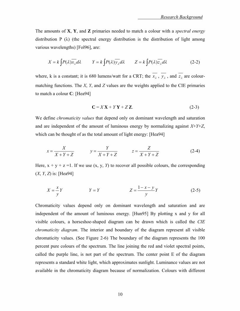


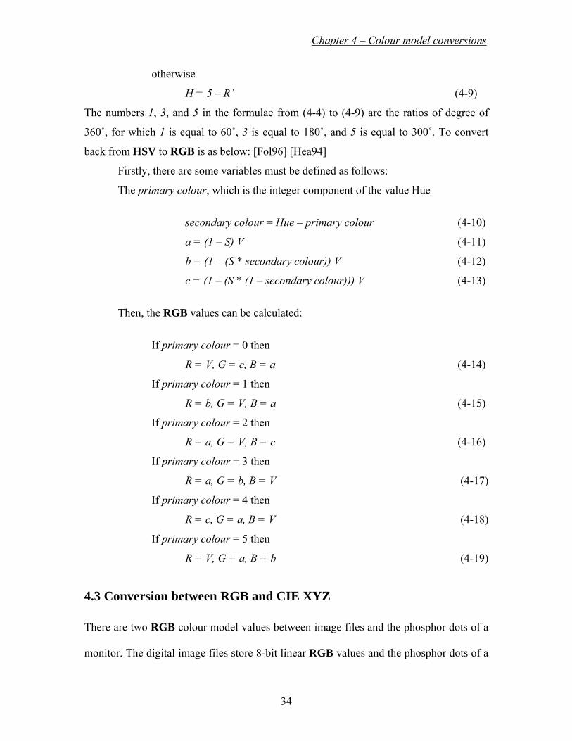


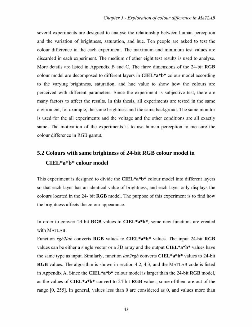


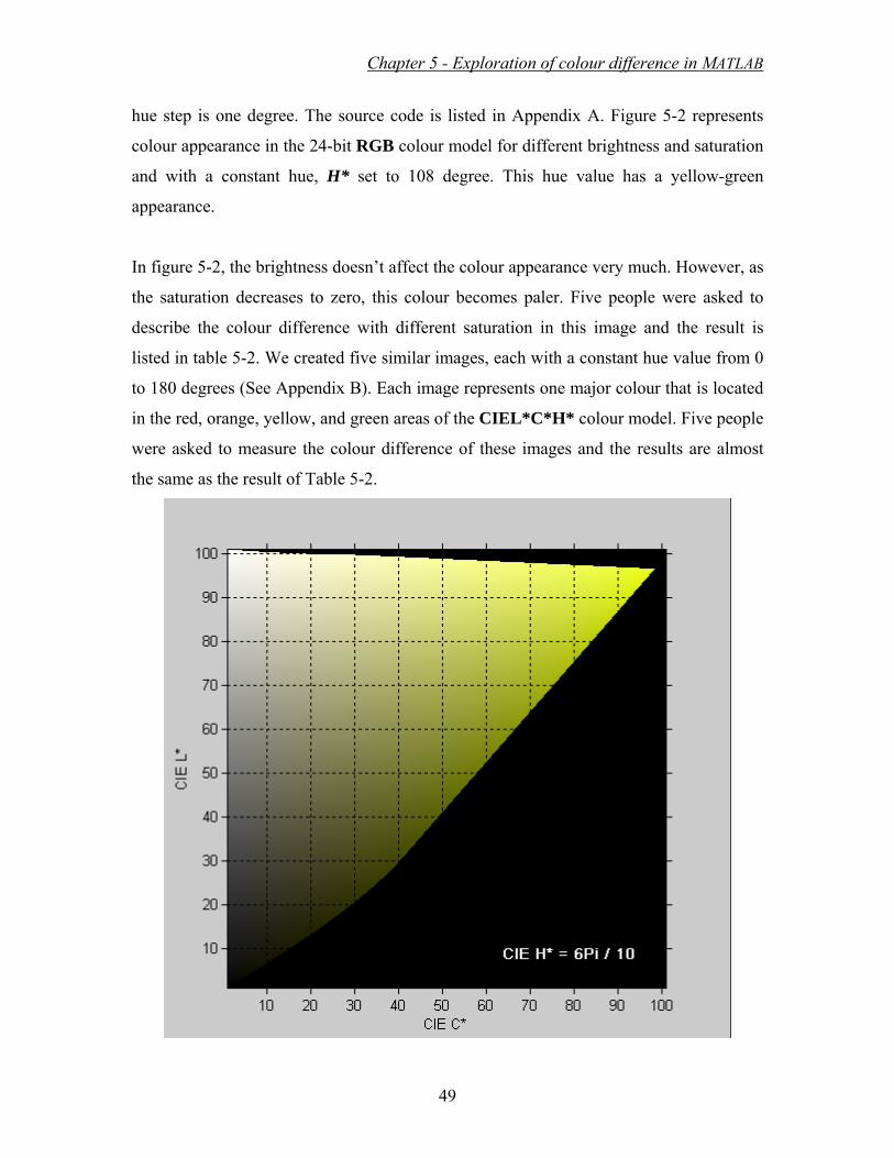


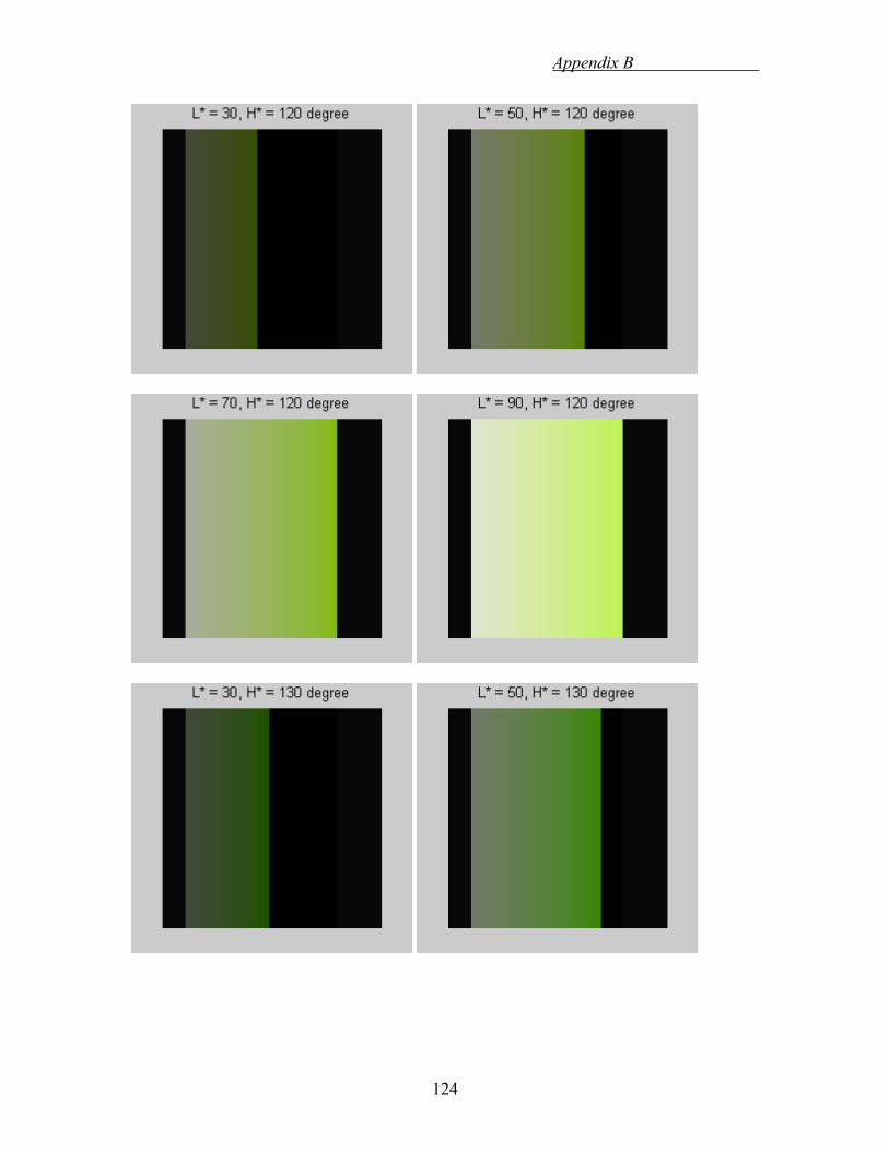


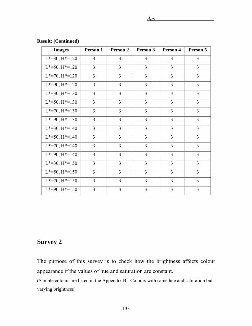


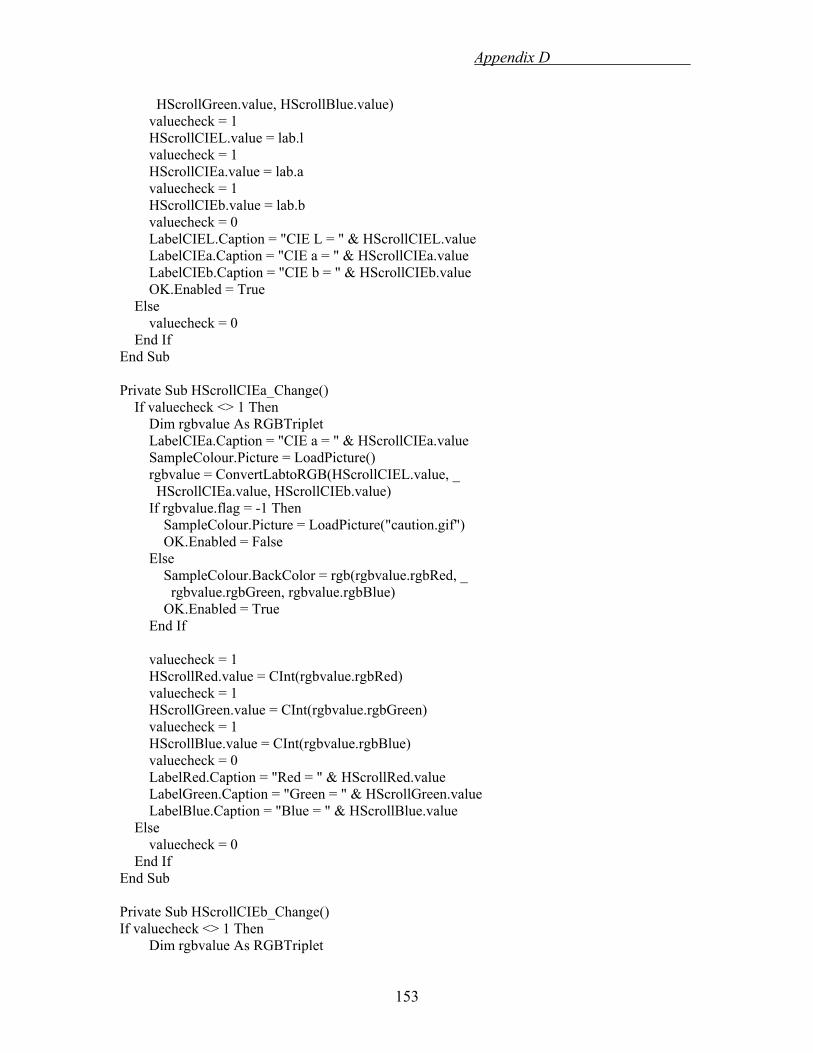


![Download or print gazette [PDF, 2.5MB] - Victoria Government Gazette](https://static.documents.pub/doc/80x56/620bbd71e638ff50200d1424/download-or-print-gazette-pdf-25mb-victoria-government-gazette.jpg)


![Brennan, M. (2011) National Curriculum: A political ...vuir.vu.edu.au/9040/1/VUIR-AJE-NationalCurric+Table[1].pdf · national curriculum: a political-educational tangle The politics](https://static.documents.pub/doc/80x56/5ba9ebc109d3f2580f8d6a9e/brennan-m-2011-national-curriculum-a-political-vuirvueduau90401vuir-aje-nationalcurrictable1pdf.jpg)


