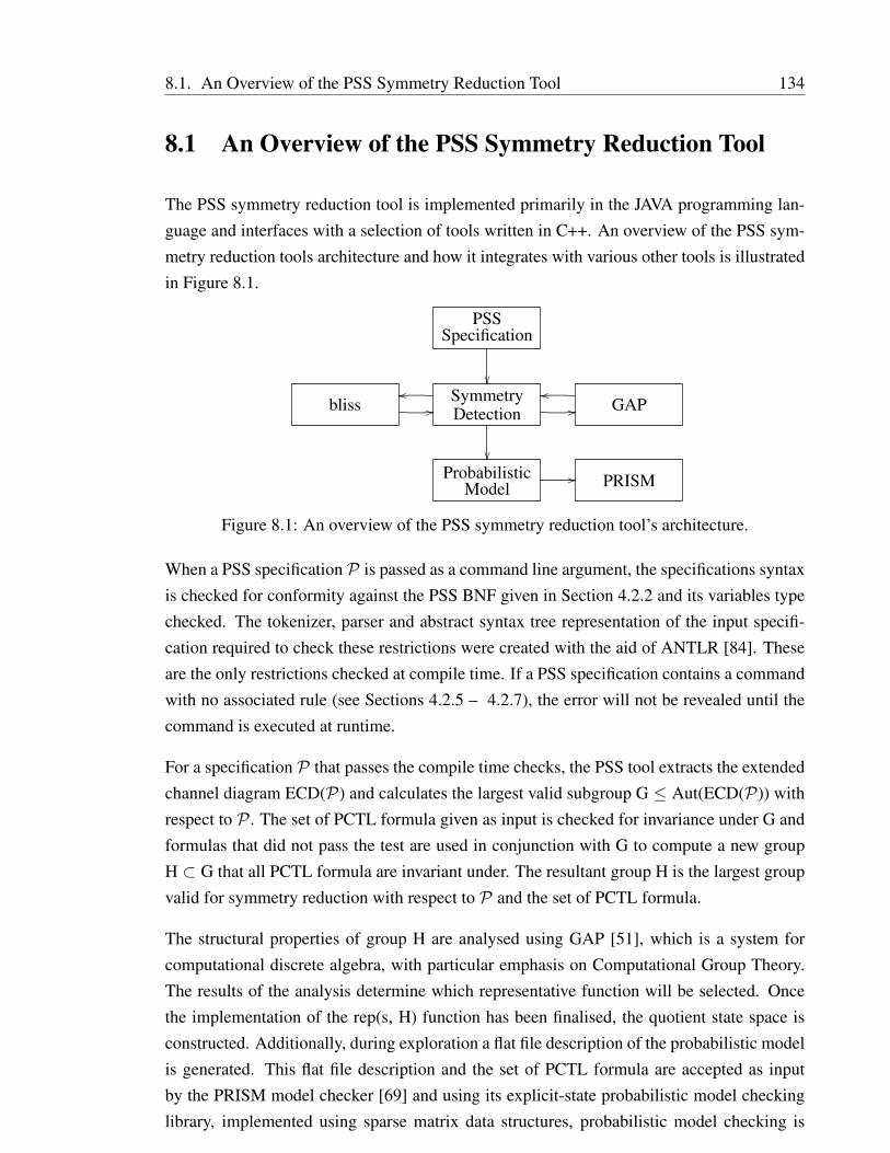
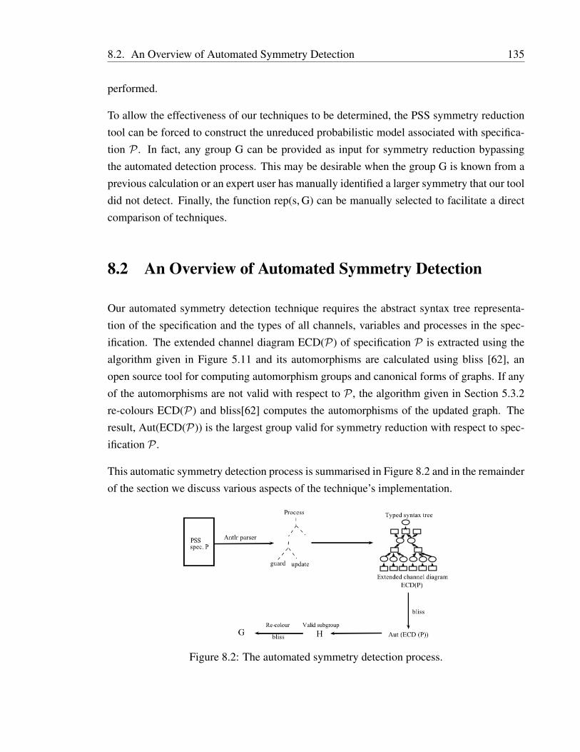
Glasgow Theses Service http://theses.gla.ac.uk/ [email protected]Power, Christopher (2012) Probabilistic symmetry reduction. PhD thesis. http://theses.gla.ac.uk/3493/ Copyright and moral rights for this thesis are retained by the author A copy can be downloaded for personal non-commercial research or study, without prior permission or charge This thesis cannot be reproduced or quoted extensively from without first obtaining permission in writing from the Author The content must not be changed in any way or sold commercially in any format or medium without the formal permission of the Author When referring to this work, full bibliographic details including the author, title, awarding institution and date of the thesis must be given
Power, Christopher (2012) Probabilistic symmetry reduction. PhD thesis. http://theses.gla.ac.uk/3493/ Copyright and moral rights for this thesis are retained by the author A copy can be downloaded for personal non-commercial research or study, without prior permission or charge This thesis cannot be reproduced or quoted extensively from without first obtaining permission in writing from the Author The content must not be changed in any way or sold commercially in any format or medium without the formal permission of the Author When referring to this work, full bibliographic details including the author, title, awarding institution and date of the thesis must be given
SUBMITTED IN FULFILMENT OF THE REQUIREMENTS FOR THE DEGREE OF
DOCTOR OF PHILOSOPHY
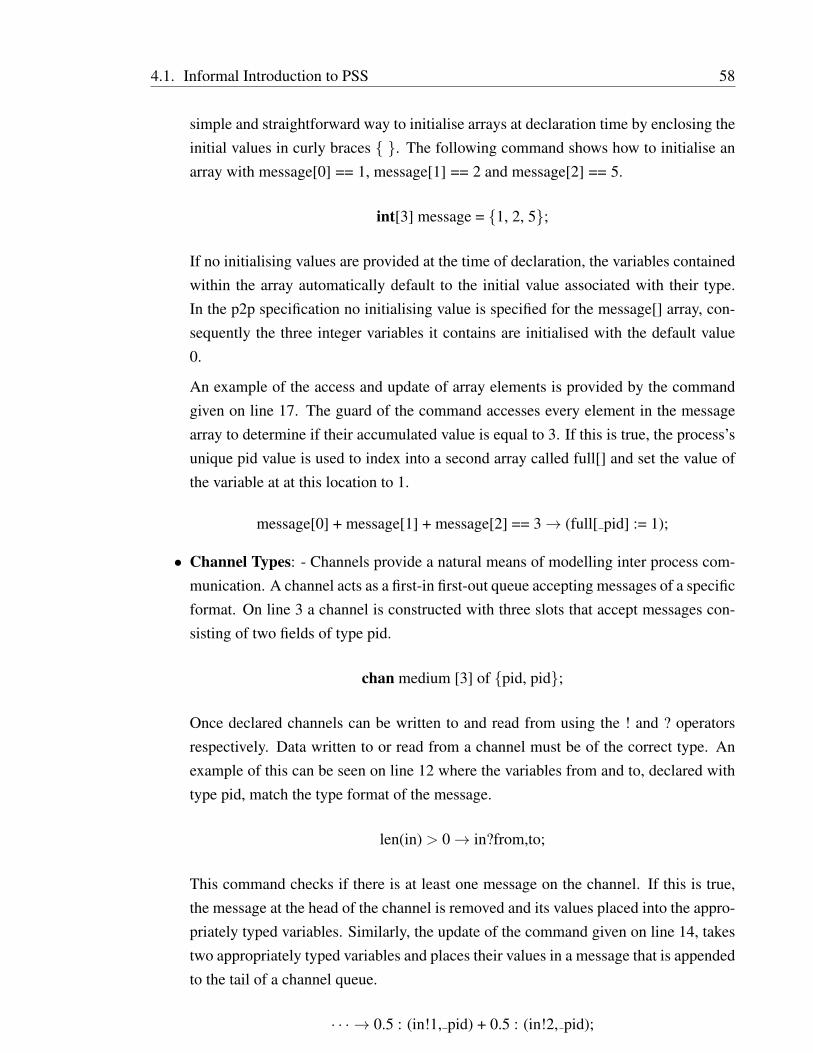
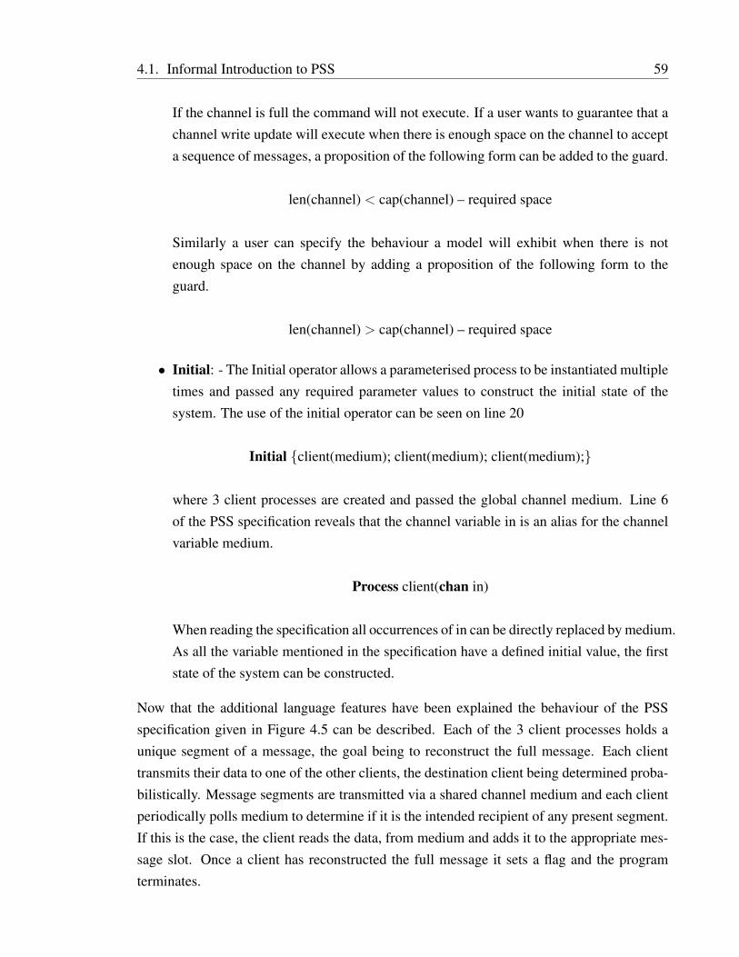
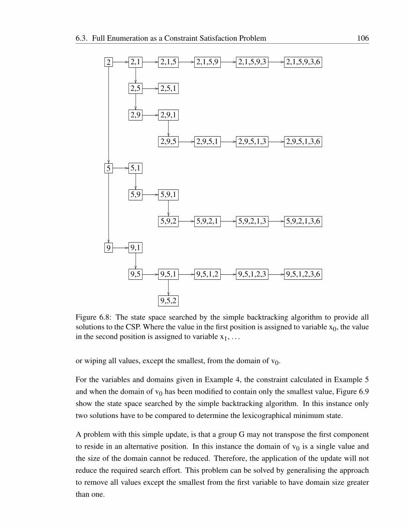
SCHOOL OF COMPUTING SCIENCE
COLLEGE OF SCIENCE AND ENGINEERING
UNIVERSITY OF GLASGOW
APRIL 2012
Abstract
Model checking is a technique used for the formal verification of concurrent systems. Amajor hindrance to model checking is the so-called state space explosion problem wherethe number of states in a model grows exponentially as variables are added. This meanseven trivial systems can require millions of states to define and are often too large to feasiblyverify. Fortunately, models often exhibit underlying replication which can be exploited to aidin verification. Exploiting this replication is known as symmetry reduction and has yieldedconsiderable success in non probabilistic verification.
The main contribution of this thesis is to show how symmetry reduction techniques canbe applied to explicit state probabilistic model checking. In probabilistic model checkingthe need for such techniques is particularly acute since it requires not only an exhaustivestate-space exploration, but also a numerical solution phase to compute probabilities or otherquantitative values.
The approach we take enables the automated detection of arbitrary data and component sym-metries from a probabilistic specification. We define new techniques to exploit the identifiedsymmetry and provide efficient generation of the quotient model. We prove the correctnessof our approach, and demonstrate its viability by implementing a tool to apply symmetryreduction to an explicit state model checker.
Acknowledgments
I would like to thank my supervisor, Alice Miller, for her time, support and advice. I wouldalso like to thank my Ph.D. examiners, David Parker and John O’Donnell. Their suggestionsgreatly enhanced my dissertation. Finally, thank you to everybody who supported me overthe last four years.
Model checking is a technique used in the formal verification of concurrent systems. To ver-ify the correctness of a system, a model of the system is generated that contains all possiblebehaviours. This set of system behaviours can then be checked against a set of properties toascertain if the system behaves as expected. Example properties include: “process 1 and pro-cess 2 are never in their critical sections simultaneously” or “it is always possible to restartthe system”.
As the model checking process has became increasingly sophisticated, the range of systemsthat can be described and verified has increased. One prevalent example is the description ofprobabilistic systems. By extending a specification language to allow for transitions betweenstates to be labelled with the likelihood that they will occur, properties such as: “the messagewill be delivered with probability 0.6” or “the probability of shutdown occurring is at most0.02” can be verified. Probabilistic model checking has the advantage of providing efficientand rigorous methods for evaluating a wide range of quantitative properties.
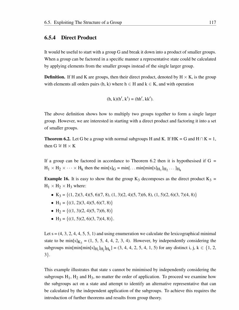
A major hindrance to model checking is the so-called state space explosion problem. Holz-mann [58] explains that although verification algorithms have a linear run time complexity,this is offset as the number of states in a model grows exponentially as variables are added.This means that even trivial real-life systems can require millions of states to define theirbehaviour.
1
2
The reason that non-probabilistic model checking has been so successful in the real worldis that an enormous amount of work has been put into developing efficient implementationtechniques. These include state compression [57], partial order reduction [52, 85], symmetryreduction [20] and symbolic storage, where states and transitions of a model are representedsymbolically (as opposed to explicitly) in order to save space [16]. These techniques haveallowed the verification of ever increasing complex systems and greatly enhanced the uptakeof model checking.
In the probabilistic domain, alleviating the state space explosion problem is an active re-search area. Techniques including symbolic storage [6, 67], partial order reduction [7, 28]and bisimulation minimisation [63] have been investigated. Furthermore, some steps havebeen made in examining the application of probabilistic symmetry reduction to symbolicallystored state-spaces [68, 31].
Symmetry reduction is a technique concerned with exploiting underlying regularities in thestate space by only storing one representative of a class of states. If symmetry is knownto be present in a model then model checking of certain properties can be performed over aquotient state-space. Importantly, symmetry reduction is implemented differently in explicit-state and symbolic model checkers, each with their own research challenges.
In explicitly represented systems the exploitation of symmetry can be highly profitable interms of time and space. Recent work has focused on providing “push button” or automaticsymmetry detection [30] and reduction in addition to widening the set of systems to whichsymmetry can be applied [94]. To our knowledge little work has been conducted on theapplication of symmetry reduction to probabilistic explicit state model checking. Therefore,we propose to investigate the application of symmetry reduction in probabilistic explicit statemodel checking. To present the results of this investigation the rest of the thesis is structuredas follows:
We provide a review of model checking and symmetry reduction literature in Chapters 2and 3 respectively and highlighted that no research has been conducted on the application ofsymmetry reduction to explicit state probabilistic model checking.
Our contribution begins in Chapter 4 where we formally defined a new probabilistic modelspecification language. The presented specification language is capable of exhibiting com-plex symmetry groups while being simple enough to allow the correctness of our detectionand reduction techniques to be proved. We make use of the language in the remainder of thethesis to aid in the presentation of our results.
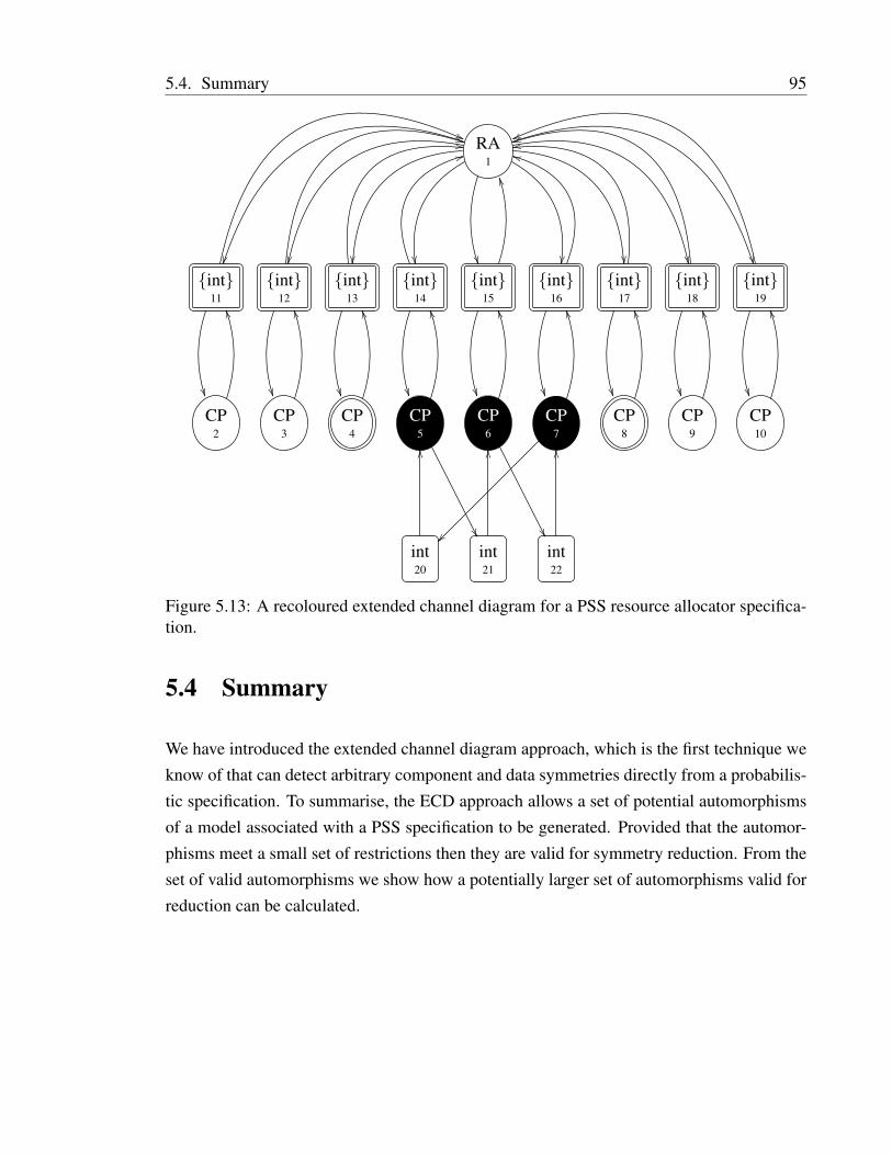
In Chapter 5 we introduced the extended channel diagram approach, which is the first tech-nique we know of that can detect arbitrary component and data symmetries directly from
3
a probabilistic specification. The approach involves computing the symmetry group of thespecification and using the presented techniques determines a subgroup of these symmetrieswhich induces automorphisms of the underlying model that are valid for symmetry reduc-tion.
In Chapter 6 we present a selection of new techniques to efficiently compute equivalenceclass representatives for certain classes of symmetry groups. We present enhancements thatimprove the average runtime of exhaustive search and where enumeration is infeasible, weconsiders a tailored made local search algorithm. For symmetry groups possessing identifi-able structural properties we provide efficient techniques that do not require the exhaustiveapplication of all elements in the symmetry group . We suggest techniques for the fully sym-metric group, cyclic groups and groups that can be decomposed as an internal direct productor as an internal semi direct product.
In Chapter 7 we consider how to combine our presented techniques to construct a smallerquotient model directly from a probabilistic specification. Finally, in Chapter 8 we describeour model checker which implements the presented specification language, detection and re-duction techniques. The model checker is used to test the viability of applying our approachof automated symmetry reduction to explicit state probabilistic model checking. For a va-riety of symmetric specifications we show significant runtime and memory savings can bemade while performing probabilistic model checking.
CHAPTER 2
Model Checking
In this chapter we present established approaches to model checking. Section 2.1 introducesthe notion of formal verification and defines the model checking process. In Section 2.2we cover some common types of models and in Section 2.3 we cover a selection of temporallogics. Issues concerning underlying data structures and key algorithms are discussed in Sec-tion 2.4 and Section 2.5 respectively. The chapter closes with a review of relevant currentlyavailable model checkers and a discussion on the state space explosion problem.
2.1 Introduction
Computerised systems have become an integral part of our lives and technological pro-gression has led to the scenario where these systems directly control safety critical appli-cations. Systems of this type include aeroplane landing systems [80], nuclear reaction man-agement [83] and medical systems [76]. In instances where human life is placed at directrisk, it is essential that controlling software functions correctly. However, even after decadesof research, the best of traditional software development methodologies cannot guarantee abug free system [60]. Furthermore, these methodologies cannot provide enough confidenceto assert if a system correctly implements its requirements specification [12].
In software and hardware design of complex or safety critical systems, the majority of time
4
2.1. Introduction 5
and cost is spent on the verification phase. This motivates research into techniques that easeverification, increasing both coverage and confidence. Formal methods is a technique thatoffers these desired attributes. Subtle errors that remain hidden after emulation, testing andsimulation can potentially be revealed using formal methods.
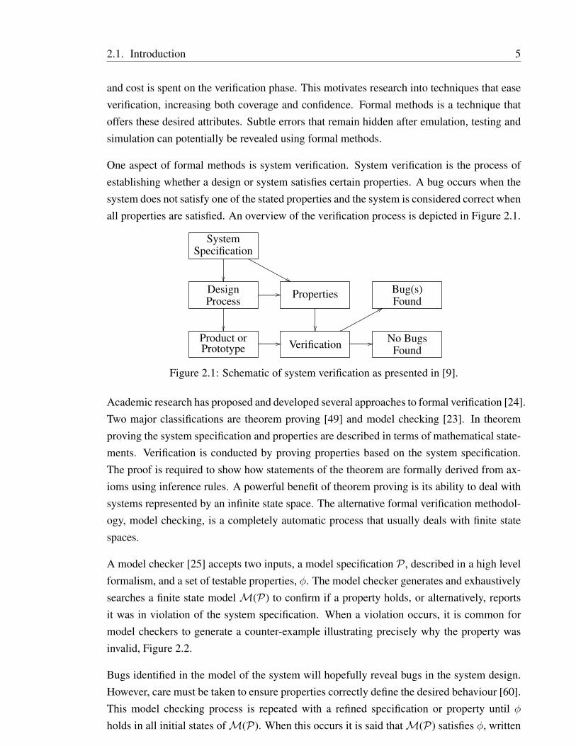
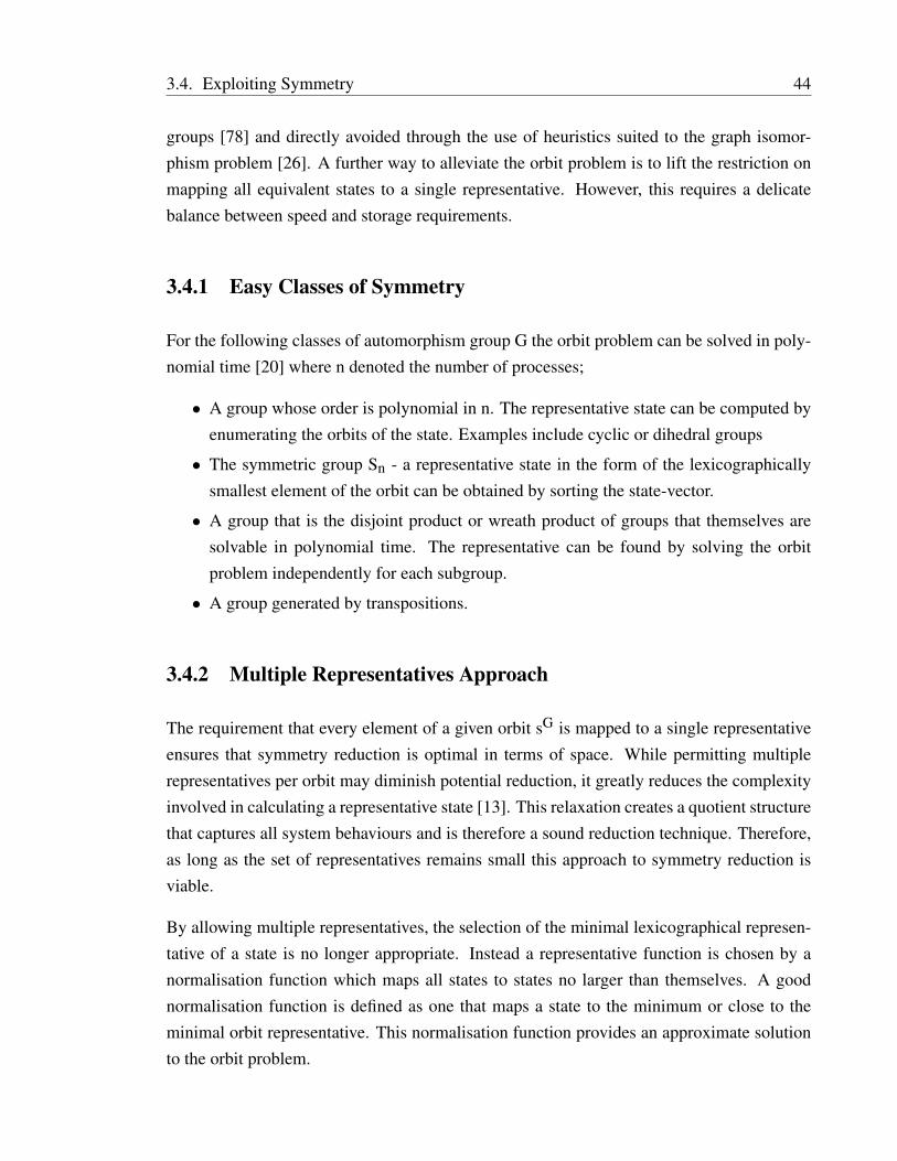
One aspect of formal methods is system verification. System verification is the process ofestablishing whether a design or system satisfies certain properties. A bug occurs when thesystem does not satisfy one of the stated properties and the system is considered correct whenall properties are satisfied. An overview of the verification process is depicted in Figure 2.1.
SystemSpecification
&&DesignProcess
// Properties
Bug(s)Found
Product orPrototype
// Verification //
88
No BugsFound
Figure 2.1: Schematic of system verification as presented in [9].
Academic research has proposed and developed several approaches to formal verification [24].Two major classifications are theorem proving [49] and model checking [23]. In theoremproving the system specification and properties are described in terms of mathematical state-ments. Verification is conducted by proving properties based on the system specification.The proof is required to show how statements of the theorem are formally derived from ax-ioms using inference rules. A powerful benefit of theorem proving is its ability to deal withsystems represented by an infinite state space. The alternative formal verification methodol-ogy, model checking, is a completely automatic process that usually deals with finite statespaces.
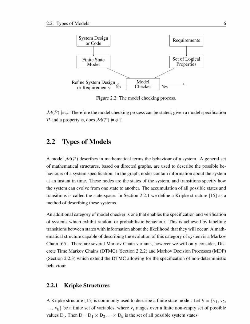
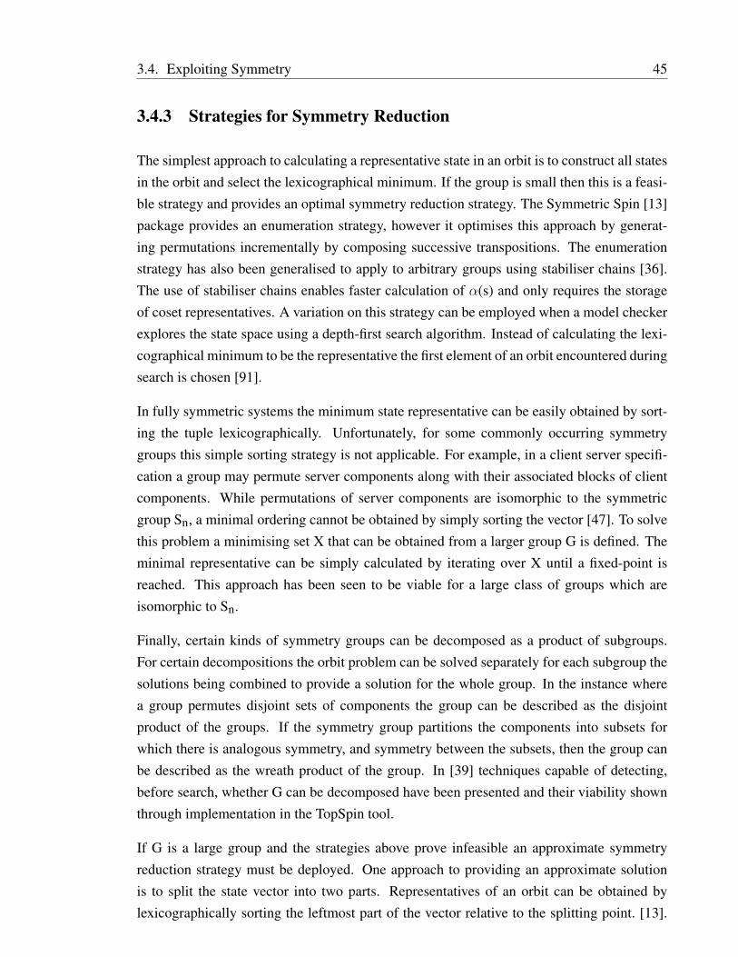
A model checker [25] accepts two inputs, a model specification P , described in a high levelformalism, and a set of testable properties, φ. The model checker generates and exhaustivelysearches a finite state modelM(P) to confirm if a property holds, or alternatively, reportsit was in violation of the system specification. When a violation occurs, it is common formodel checkers to generate a counter-example illustrating precisely why the property wasinvalid, Figure 2.2.
Bugs identified in the model of the system will hopefully reveal bugs in the system design.However, care must be taken to ensure properties correctly define the desired behaviour [60].This model checking process is repeated with a refined specification or property until φholds in all initial states ofM(P). When this occurs it is said thatM(P) satisfies φ, written
2.2. Types of Models 6
System Designor Code
Requirements
Finite State
Model
((
Set of LogicalProperties
ww
Refine System Designor Requirements
ModelChecker Yes
//Nooo
Figure 2.2: The model checking process.
M(P) |= φ. Therefore the model checking process can be stated; given a model specificationP and a property φ, doesM(P) |= φ ?
2.2 Types of Models
A modelM(P) describes in mathematical terms the behaviour of a system. A general setof mathematical structures, based on directed graphs, are used to describe the possible be-haviours of a system specification. In the graph, nodes contain information about the systemat an instant in time. These nodes are the states of the system, and transitions specify howthe system can evolve from one state to another. The accumulation of all possible states andtransitions is called the state space. In Section 2.2.1 we define a Kripke structure [15] as amethod of describing these systems.
An additional category of model checker is one that enables the specification and verificationof systems which exhibit random or probabilistic behaviour. This is achieved by labellingtransitions between states with information about the likelihood that they will occur. A math-ematical structure capable of describing the evolution of this category of system is a MarkovChain [65]. There are several Markov Chain variants, however we will only consider, Dis-crete Time Markov Chains (DTMC) (Section 2.2.2) and Markov Decision Processes (MDP)(Section 2.2.3) which extend the DTMC allowing for the specification of non-deterministicbehaviour.
2.2.1 Kripke Structures
A Kripke structure [15] is commonly used to describe a finite state model. Let V = v1, v2,. . ., vk be a finite set of variables, where vi ranges over a finite non-empty set of possiblevalues Di. Then D = D1 × D2 . . .× Dk is the set of all possible system states.
2.2. Types of Models 7
Definition. A Kripke structureM over D is a tupleM = (S, S0, R) where:• S = D is a non-empty finite set of states.
• S0 ⊆ S is a set of initial states.
• R ⊆ S× S is a transition relation.
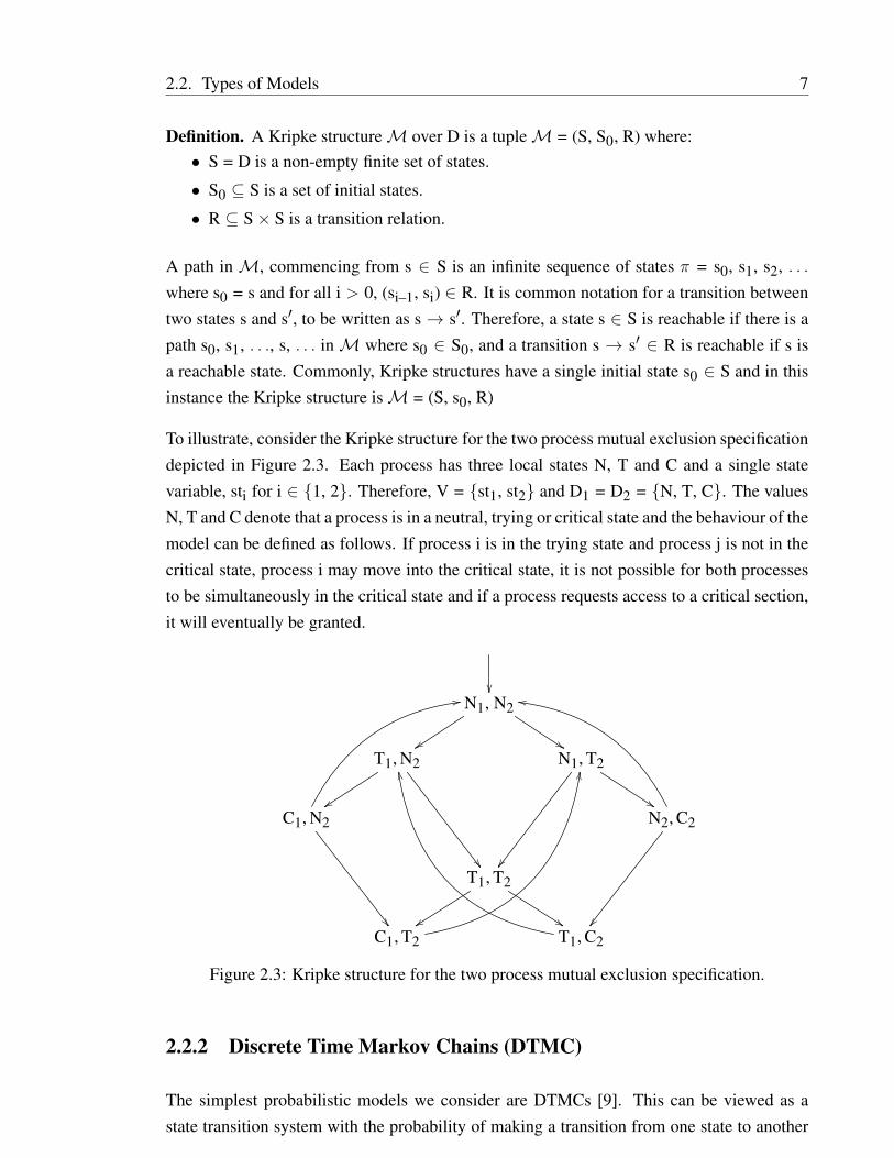
A path inM, commencing from s ∈ S is an infinite sequence of states π = s0, s1, s2, . . .where s0 = s and for all i > 0, (si–1, si) ∈ R. It is common notation for a transition betweentwo states s and s′, to be written as s → s′. Therefore, a state s ∈ S is reachable if there is apath s0, s1, . . ., s, . . . inM where s0 ∈ S0, and a transition s → s′ ∈ R is reachable if s isa reachable state. Commonly, Kripke structures have a single initial state s0 ∈ S and in thisinstance the Kripke structure isM = (S, s0, R)
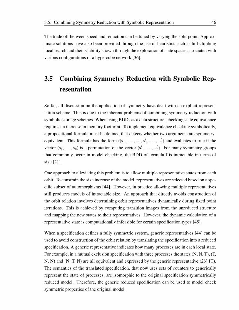
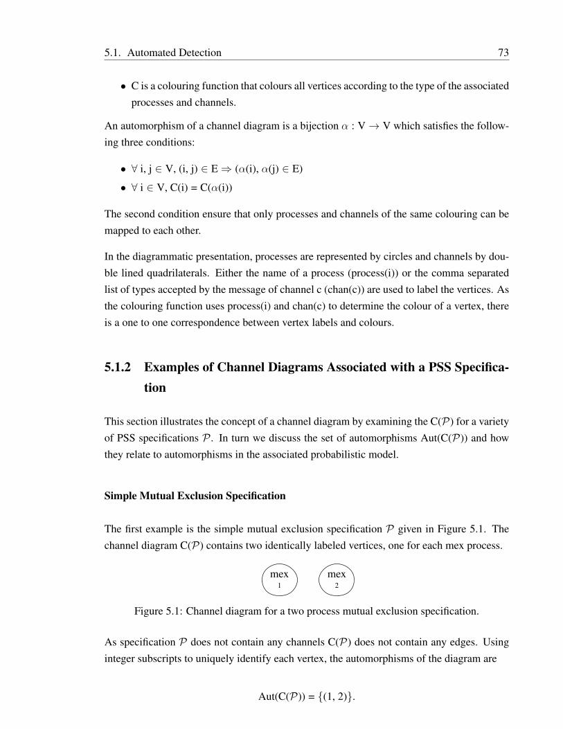
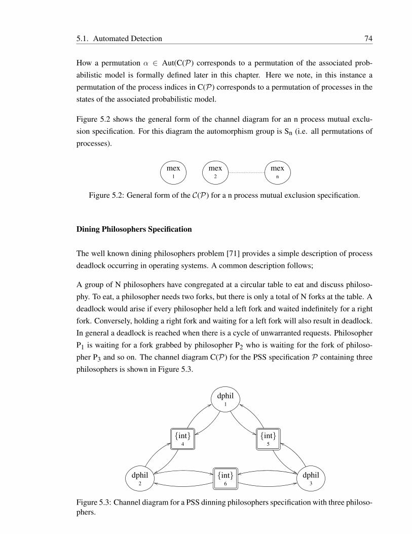
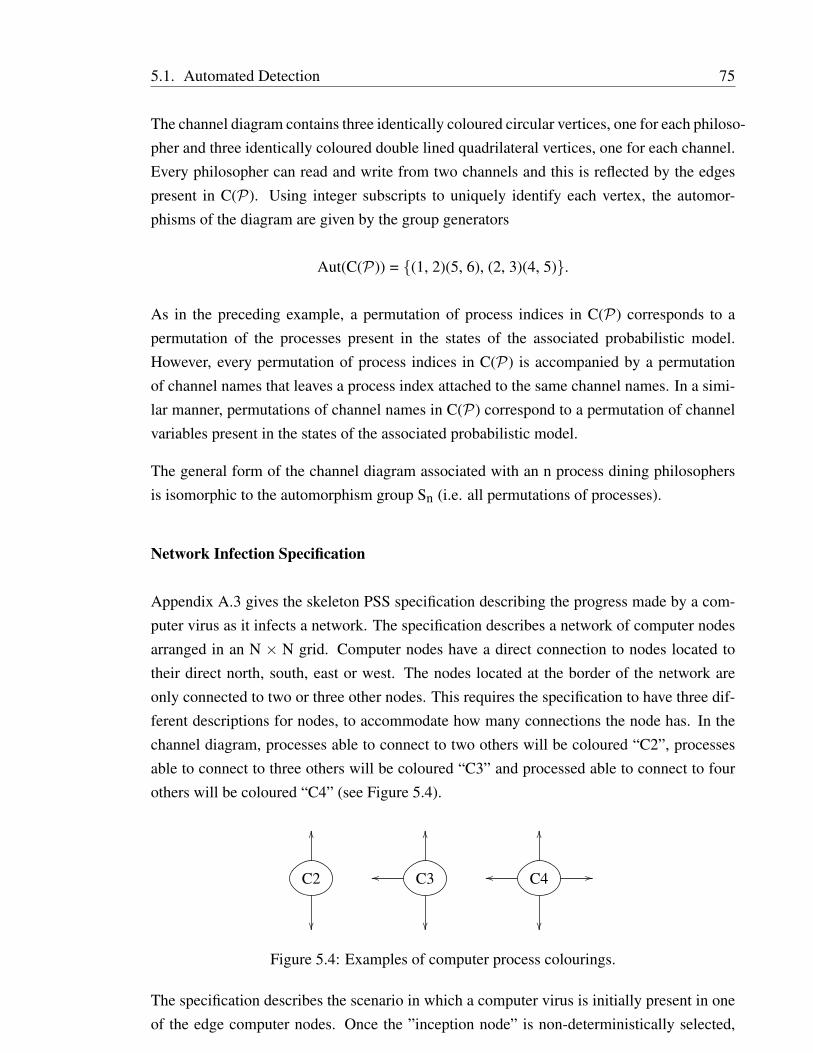
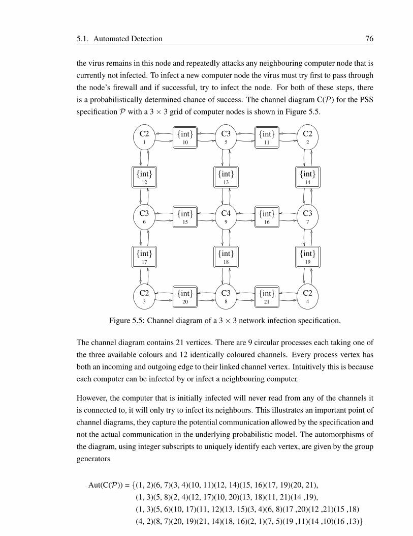
To illustrate, consider the Kripke structure for the two process mutual exclusion specificationdepicted in Figure 2.3. Each process has three local states N, T and C and a single statevariable, sti for i ∈ 1, 2. Therefore, V = st1, st2 and D1 = D2 = N, T, C. The valuesN, T and C denote that a process is in a neutral, trying or critical state and the behaviour of themodel can be defined as follows. If process i is in the trying state and process j is not in thecritical state, process i may move into the critical state, it is not possible for both processesto be simultaneously in the critical state and if a process requests access to a critical section,it will eventually be granted.
N1, N2
%%yyT1, N2
yy
N1, T2
%%C1, N2
11
N2, C2
mm
T1, T2
yy %%C1, T2
MM
T1, C2
RR
Figure 2.3: Kripke structure for the two process mutual exclusion specification.
2.2.2 Discrete Time Markov Chains (DTMC)
The simplest probabilistic models we consider are DTMCs [9]. This can be viewed as astate transition system with the probability of making a transition from one state to another
2.2. Types of Models 8
appended. As before, V = v1, v2, . . . , vk is the finite set of variables each ranging over adomain Di and D = D1 × D2 . . . ×Dk is the set of all possible system states.
Definition. A Discrete Time Markov Chain D over D is a tupleM = (S, iinit, P) where:
• S = D is a non-empty finite set of states.
• iinit : S→ [0, 1] is an initial distribution, such that∑
s∈S iinit(s) = 1.
• P : S× S→ [0, 1] is a transition probability matrix such that for all states s ∈ S∑s′∈S
P(s, s′) = 1.
An entry in transition probability matrix P(s, s′) determines the probability of moving be-tween state s and state s′. The states s′ for which P(s, s′) > 0 are possible successors tos. Therefore,
∑s′∈S P(s, s′) = 1 for all states s ∈ S. To meet the requirement,
∑s′∈S P(s,
s′) = 1 for all states s ∈ S, all terminating states are appended with a transition to themselveswith probability 1. The value iinit(s) designates the probability of the system beginning instate s. States s, with iinit(s) > 0 are the initial states of the system. Commonly DTMCs havea single initial state s0 ∈ S and in this instance the DTMC is defined D = (S, s0, P)
A path π in D starting from s0 is a non-empty sequence of states s0, s1, s2, . . . where si ∈ Sand P(si, si+1) > 0 for all i≥ 0. The execution path π can be finite, πfin, or infinite, πinf, withthe ith state being denoted π(i). The notation Path(s) is the set of all path fragments initiatingfrom the state s. Possible evolutions of the system are represented by paths. Therefore,to reason about the behaviour of the system, the probability that a path is taken must becalculated. For each state s ∈ S a probability measure Probs on Path(s) is defined. Tofacilitate this P(πfin) = 1 where πfin = s0 and P(πfin) = P(s0, s1) · P(s1, s2) · · · P(sn–1, sn)where πfin = s0, s1, . . . , sn.
The cylinder set C(πfin) is the set of all paths with prefix πfin and∑
s is the smallest σ-algebra 1 on Path(s) containing all the sets C(πfin). The probability measure Probs on
∑s is
the unique measure such that Probs(C(πfin)) = P(πfin). The probability of a system exhibitinga specific behaviour can be calculated by identifying the set of paths satisfying the conditionand imposing upon them the measure Probs.
2.2.3 Markov Decision Processes (MDP)
MDPs [9] provide a mathematical framework for modelling decisions in situations whereoutcomes are partly random and partly under the control of the decision maker. An MDP is
1A π-algebra is a pair (Outc, ε) where Outc is a nonempty set and ε ⊂ 2Outc a set consisting of subsets ofOutc that contains the empty set and is closed under complementation and countable unions.
2.2. Types of Models 9
useful in the context of model checking as it allows the description of a number of probabilis-tic systems operating in parallel. Furthermore, non-deterministic transitions can be specifiedwhen the exact probability distribution is unknown, or irrelevant. , let V and D follow thesame definition as given for Kripke structures and DTMCs.
Definition. A Markov Decision ProcessM over D is a tupleM = (S, iinit, Steps) where:• S = D is a non-empty finite set of states.
• iinit : S→ [0, 1] is an initial distribution, such that∑
s∈S iinit(s) = 1.
• Steps : S→ 2Dist(s) is a transition function.
The definition is similar to that of a DTMC but transition probability matrix P is replacedby Steps. For a state s ∈ S, Steps(s) is the set of non-deterministic choices available ins. Specifically, Steps(s) is a function mapping states onto a finite, non-empty subset ofprobability distributions and takes the form µ : S→ [0, 1] where
∑s∈S µ(s) = 1.
An execution path through an MDP is a non-empty sequence s0µ1–––→ s1
µ2–––→ . . . wheresi ∈ S, µi+1 ∈ Steps(si) and µi+1(si+1) > 0 for all i ≥ 0. In keeping with the notationpresented for a DTMC, πfin is a finite execution path, πinf an infinite path and the ith state ofa path denoted π(i). The notation Path(s) is the set of all path fragments initiating from thestate s.
An execution path of an MDP requires both non-deterministic and probabilistic transitionsto be resolved. Non-deterministic choices are made by an adversary where the decisionis determined by the choices made in all previous runs. An adversary A can be definedformally as a function that maps every finite path πfin in an MDP onto a distribution A(πfin) ∈Steps(last(πfin)) where last(πfin) is the final state of the finite path. For convenience the subsetof Path(s) which corresponds to adversary A is denoted PathA(s).
The behaviour of the MDP for an adversary A is probabilistic in nature. It can thereforebe defined by a DTMC where the probability of non-deterministic transitions are given bya probability distribution selected by A. Drawing conclusions about an MDP’s behaviourfor a given adversary is meaningless. Meaningful results, in the form of maximum andminimum probabilities can be ascertained by computing over all possible adversaries. Whencomputing the maximum or minimum probability for an observed event it is often beneficialto use adversaries with a notion of fairness. For example, in a non-deterministic schedulerit is impossible to draw meaningful conclusions if every process does not eventually get achance to proceed. A path π is fair, if for states s occurring infinitely often in π each choiceµ ∈ Steps(s) is taken infinitely often. Additionally, an adversary A is fair if ProbA
s (π ∈PathA(s) π is fair) = 1 for all s ∈ S.
2.3. Temporal Logic 10
2.3 Temporal Logic
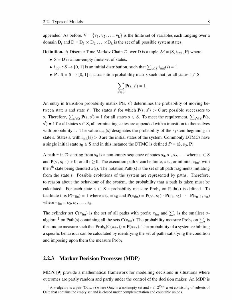
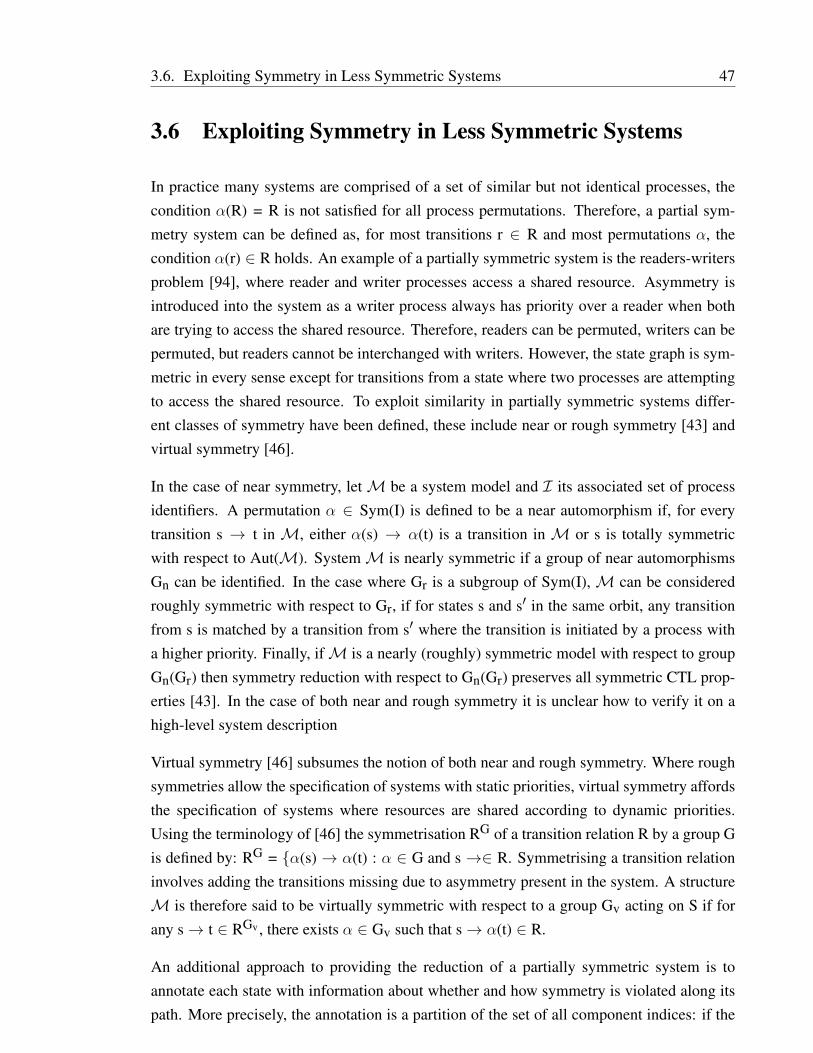
It is common for the set of testable properties φ to be expressed using a temporal logic. Tem-poral logics provide a formal language to reason about the behavioural properties of parallelprograms and more generally reactive systems. Their application in Computing Science waspioneered by Pnueli [87] who argued that existing techniques for verification were not ade-quate for concurrent, reactive systems. Temporal logics alleviated this issue by allowing theuser to reason about related events at different moments in a system’s execution. Temporallogic formalisms may be classified according to their particular view of time; Linear Timewhere for every given path every state has a unique successor, and Branching Time, whereevery state has several successors, Figure 2.4.
A
A
A
A
B
B
C
B
C
D
E
F
D
E
F
G B D G B D
Figure 2.4: Comparative views of time in temporal logics.
2.3.1 Linear Time Temporal Logic (LTL)
Linear Time Temporal Logic [87] allows the future behaviour of a system to be reasonedabout. A collection of paths represent the set of possible future behaviours, any one of whichmight be the actual outcome of the systems execution. To aid in behavioural descriptions aset of atoms, which state facts that may hold in a system are used. The choice of atoms isdependent on the system being described but general examples include “Queue 4 is full” and“Process 3 is active”.
Linear Time Temporal Logic, where φ is the formula and p is any propositional atom from aset of atoms, has the following syntax in Backus Naur Form:
φ := > ⊥ p ¬φ φ ∧ φ φ ∨ φ φ→ φ X φ F φ G φ φ U φ φ W φ
φ R φ
The symbols X, F, G, U, R, and W are temporal connectives where X reasons about the nextstate, F some future state and G all future states. Symbols U, R and W are known as Until,
2.3. Temporal Logic 11
Release and Weak-until, respectively. Take a Kripke structureM and a path π = s0, s1, s2,. . . . Whether π satisfies a LTL formula is defined by the satisfaction relation |=. For the pathπ we define s0 as the first state in the path and, for all i ≥ 0, πi is the suffix of π starting fromstate si. The relation |= is defied inductively below;
• π |= >.
• π 6|= ⊥.
• π |= p iff p is true in s0.
• π |= ¬φ iff π 6|= φ.
• π |= φ1 ∧ φ2 iff π |= φ1 and π |= φ2.
• π |= φ1 ∨ φ2 iff π |= φ1 or π |= φ2.
• π |= φ1 → φ2 iff π |= φ2 whenever π |= φ1.
• π |= X φ iff π1 |= φ.
• π |= G φ iff, for all i ≥ 1 πi |= φ.
• π |= F φ iff, there is some i ≥ 1 such that πi |= φ.
• π |= φ U ψ iff, there is some i ≥ 1 such that πi |= ψ and for all j = 1, . . . , i – 1 we haveπj |= φ.
• π |= φ W ψ iff, either there is some i ≥ 1 such that πi |= ψ and for all j = 1, . . . , i – 1we have πj |= φ, or for all k ≥ 1 we have πk |= φ.
• π |= φ R ψ iff, either there is some i ≥ 1 such that πi |= φ and for all j = 1, . . . , i – 1we have πj |= ψ, and for all k ≥ 1 we have πk |= ψ.
Therefore, take a Kripke structureM, s ∈ S and a LTL formula φ. We writeM,s |= φ. if,for every execution path π ofM starting at s, we have π |= φ.
Example LTL Properties
Referring to the Kripke structure for the mutual exclusion problem defined in Figure 2.3 anattempt to verify the correctness of the solution can be made by checking it against a set ofLTL properties:
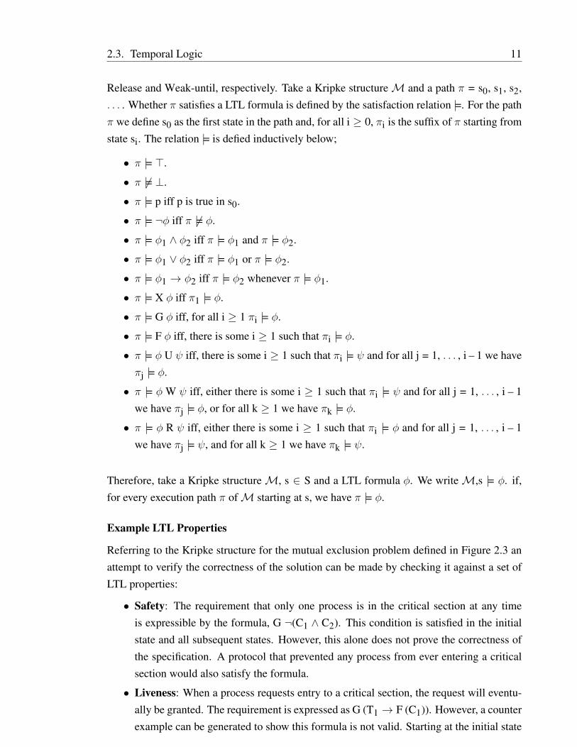
• Safety: The requirement that only one process is in the critical section at any timeis expressible by the formula, G ¬(C1 ∧ C2). This condition is satisfied in the initialstate and all subsequent states. However, this alone does not prove the correctness ofthe specification. A protocol that prevented any process from ever entering a criticalsection would also satisfy the formula.
• Liveness: When a process requests entry to a critical section, the request will eventu-ally be granted. The requirement is expressed as G (T1 → F (C1)). However, a counterexample can be generated to show this formula is not valid. Starting at the initial state
2.3. Temporal Logic 12
there is a path where T1 becomes true but C1 remains false, N1, N2 → T1, N2 →T1, T2 → T1, C2 → T1, N2 → . . . . This path arises as the state T1, T2, where bothprocesses are in a trying state gives a choice of which process moves to the criticalsection. This problem can be alleviated by remodelling the system to allow the stateT1, T2 to appear twice in the transition system. Each occurrence implicitly indicatingwhich process will proceed to a critical state.
• Non-blocking: A process can always request entry to its critical section. For example,in process one we would like to attest that for every state satisfying N1, there is asuccessor satisfying T1. However, statements of this nature are not expressible in LTLas the logic does not contain an existence quantifier on paths.
2.3.2 Computation Tree Logic (CTL)
Computation Tree Logic [19], is a branching-time logic, meaning that its model of timeis a tree-like structure in which the future is not determined. CTL provides the previouslycovered LTL temporal operators U, F, G and X in addition to new quantifiers A and E. Thesequantifiers express All paths, and Exists a path, respectively. This allows properties such as,“there is a reachable state satisfying q” or “from all reachable states satisfying p, it is possibleto maintain p continuously until reaching a state satisfying q” to be expressed.
CTL, where φ is the state formula and p is any propositional atom from a set of Atoms, hasthe following syntax in Backnus Naur Form:
φ := > ⊥ p ¬φ φ ∧ φ φ ∨ φ φ→ φ AX φ EX φ AF φ EF φ AG φ
EG φ A [φ U φ] E [φ U φ]
CTL temporal connectives are formed from a pair of symbols that are indivisible, the firstbeing either an A or E and the second being one of the connectives X, F, G, or U. Thesymbols X, F, G and U cannot occur without being preceded by an A or an E and similarly,every A or E must be accompanied by X, F, G and U.
For a Kripke structureM, a state s ∈ S and a CTL formula φ, the relationM, s |= φ can bedefined by structural induction on φ in the following manner:
• M,s |= >.
• M,s 6|= ⊥.
• M,s |= p if p is true in s.
• M,s |= ¬φ iffM, s 6|= φ.
• M,s |= φ1 ∧ φ2 iffM, s |= φ1 andM, s |= φ2.
2.3. Temporal Logic 13
• M,s |= φ1 ∨ φ2 iffM, s |= φ1 orM, s |= φ2.
• M,s |= φ1 → φ2 iffM,s 6|= φ1 orM,s |= φ2.
• M,s |= AX φ iff for all s1 such that s→ s1 we haveM,s1 |= φ.
• M,s |= EX φ iff for some s1 such that s→ s1 we haveM,s1 |= φ.
• M,s |= AG φ iff for all paths s1 → s2 → s3 → ... where s1 equals s, and all si alongthe path we haveM,si |= φ.
• M,s |= EG φ iff there is a path s1 → s2 → s3 → ... where s1 equals s, and for all si
along the path we haveM,si |= φ.
• M,s |= AF φ if for all paths s1 → s2 → ... where s1 equals s, there is some si, suchthatM,si |= φ.
• M,s |= EF φ iff there is a path s1 → s2 → s3 → ... where s1 equals s, and for all si
along the path we haveM,si |= φ.
• M,s |= A [ φ1 U φ2 ] iff for all path s1 → s2 → s3 → ... where s1 equals s, that pathsatisfies φ1 U φ2.
• M,s |= E [ φ1 U φ2 ] iff there is a path s1 → s2 → s3 → ... where s1 equals s, and thatpath satisfies φ1 U φ2.
Example CTL Properties
Referring to the Kripke structure for the mutual exclusion problem defined in Figure 2.2,we can attempt to check the correctness of the solution by verifying it against a set of CTLproperties:
• Safety: The requirement that only one process is in the critical section at any time isexpressed by the formula, AG (¬(C1 ∧ C2)). This condition is satisfied in the initialstate and all subsequent states. As with LTL this formula does not cover a protocolthat prevents all processes from ever entering the critical section.
• Liveness: Having reached its trying region a process will eventually progress to itscritical section. For process one the formula AG (T1 → AF (C1))) would assert thisproperty. A counter example to this property would be, starting at the initial state, apath where T1 is true and C1 is false, N1, N2→ T1, N2→ C1, N2→ N1, N2→ . . .
• Non-blocking: A final consideration is that a process can always request entry to itscritical section. For process one an appropriate formula would be AG (N1→ EX (T1)).
2.3.3 CTL?
The Computational tree logic [48] CTL?, combines the operators of both branching andlinear time logics. The expressive power of LTL and CTL is combined, by removing the
2.3. Temporal Logic 14
constraint that temporal operators X, U, F and G have to be associated with path quantifiersA and E. In fact path quantifiers can be associated with any possible combination of linearoperators. The syntax of CTL? involves two classes of formulae: state formulae, which areevaluated in states where p is any atomic formulae and α any path formula
φ := > p ¬φ φ ∧ φ A[α] E[α]
and path formulae, which are evaluated along paths where φ is any state formula
α := φ ¬α α ∧ α α U α G α F α X α
CTL? is more expressive than LTL and CTL. It enables properties such as, “along all paths,either p is true until r, or q is true until r” (A [(p U e) ∨ (q U r)]) to be expressed. Furthermore,the logics of LTL and CTL are both subsets of CTL?. This may be surprising as LTL doesnot include the path operators A and E. However, in LTL we implicitly consider all paths fora given formula α and this is semantically equivalent to the CTL? formula A[α].
Expressive powers of LTL, CTL and CTL?.
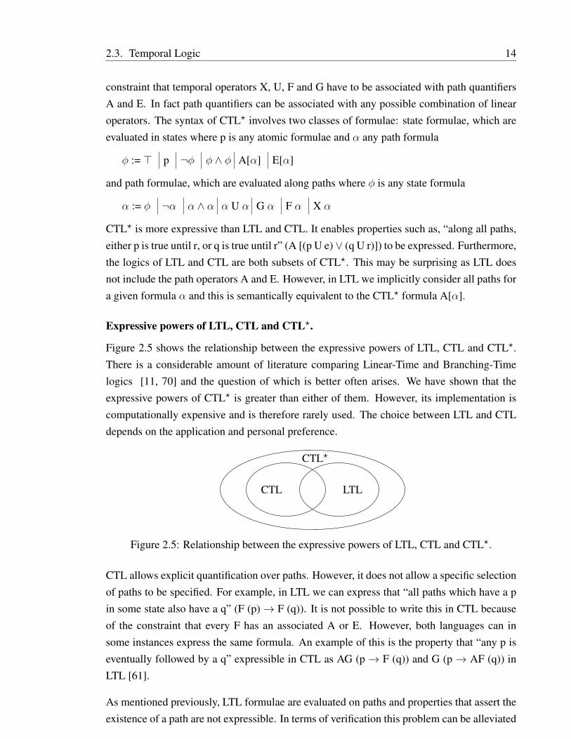
Figure 2.5 shows the relationship between the expressive powers of LTL, CTL and CTL?.There is a considerable amount of literature comparing Linear-Time and Branching-Timelogics [11, 70] and the question of which is better often arises. We have shown that theexpressive powers of CTL? is greater than either of them. However, its implementation iscomputationally expensive and is therefore rarely used. The choice between LTL and CTLdepends on the application and personal preference.
CTL LTL
CTL?
Figure 2.5: Relationship between the expressive powers of LTL, CTL and CTL?.
CTL allows explicit quantification over paths. However, it does not allow a specific selectionof paths to be specified. For example, in LTL we can express that “all paths which have a pin some state also have a q” (F (p)→ F (q)). It is not possible to write this in CTL becauseof the constraint that every F has an associated A or E. However, both languages can insome instances express the same formula. An example of this is the property that “any p iseventually followed by a q” expressible in CTL as AG (p→ F (q)) and G (p→ AF (q)) inLTL [61].
As mentioned previously, LTL formulae are evaluated on paths and properties that assert theexistence of a path are not expressible. In terms of verification this problem can be alleviated
2.3. Temporal Logic 15
by considering the complement property [61]. However, a property that contains universaland existential path quantifiers in general cannot be expressed using this approach.
2.3.4 Probabilistic Computational Tree Logic (PCTL)
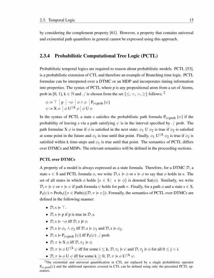
Probabilistic temporal logics are required to reason about probabilistic models. PCTL [53],is a probabilistic extension of CTL and therefore an example of Branching time logic. PCTLformulae can be interpreted over a DTMC or an MDP and incorporates timing informationinto properties. The syntax of PCTL where p is any propositional atom from a set of Atoms,prob in [0, 1], k ∈ N and ./ is chosen from the set ≤, <, >, ≥ follows; 2
φ := > p ¬φ φ ∧ φ P./prob [ψ]ψ := X φ φ U≤k φ φ U φ
In the syntax of PCTL a state s satisfies the probabilistic path formula P./prob [ψ] if theprobability of leaving s via a path satisfying ψ is in the interval specified by ./ prob. Thepath formulae X φ is true if φ is satisfied in the next state; φ1 U φ2 is true if φ2 is satisfiedat some point in the future and φ1 is true until that point. Finally, φ1 U≤k φ2 is true if φ2 issatisfied within k time-steps and φ1 is true until that point. The semantics of PCTL differsover DTMCs and MDPs. The relevant semantics will be defined in the proceeding sections.
PCTL over DTMCs
A property of a model is always expressed as a state formula. Therefore, for a DTMC D, astate s ∈ S and PCTL formula φ, we write D, s |= φ or s |= φ to say that φ holds in s. Theset of all states in which φ holds s ∈ S s |= φ is denoted Sat(φ). Similarly, we writeD, π |= ψ or π |= ψ if path formula ψ holds for path π. Finally, for a path φ and a state s ∈ S,Ps(ψ) = Probs(π ∈ Path(s) D, π |= ψ). Formally, the semantics of PCTL over DTMCs aredefined in the following manner:
• D, s |= >.
• D, s |= p if p is true in D, s.
• D, s |= ¬φ iff D, s 6|= φ.
• D, s |= φ1 ∧ φ2 iff D, s |= φ1 and D, s |= φ2.
• D, s |= P./prob [ψ] iff Ps(ψ) ./ prob.
• D, π |= X φ iff D, π1 |= φ.
• D, π |= φ U≤k ψ iff for some i ≤ k, D, πi |= ψ and D, πj |= φ for all 0 ≤ j < i.
• D, π |= φ U ψ iff for some k ≥ 0, D, π |= φ U≤k ψ.2The existential and universal quantification in CTL are replaced by a single probabilistic operator
P./ prob[ψ] and the additional operators covered in CTL can be defined using only the presented PCTL op-erators.
2.4. Storage Schemes 16
PCTL over MDPs
In the instance of MDPs the semantic definition of a path formula is identical to that ofDTMCs. However, the probability of a set of paths differs as it can only be computed fora specific adversary. Given an MDP M, the probability of a path from s satisfying pathformula ψ under adversary A is denoted PA
s (ψ) = ProbAs (π ∈ PathA(s)M, π |= ψ). To
formally define the semantics of the PCTL formula P./prob [ψ] a set of adversaries Adv isselected and quantified over. It follows that the satisfaction relation is parameterised by Adv.Therefore, a state s satisfies the formula P./prob [ψ] if PA
s (ψ) ./ prob for all adversariesA ∈ Adv. Formally the semantics of PCTL over MDPs are defined in the following manner:
• M, s |=Adv >.
• M, s |=Adv p if p is true inM, s.
• M, s |=Adv ¬φ iffM, s 6|=Adv φ.
• M, s |=Adv φ1 ∧ φ2 iffM, s |=Adv φ1 andM, s |=Adv φ2.
• M, s |= P./prob[ψ] iff PAs (ψ) ./ prob for all A ∈ Adv.
• M, π |=Adv X φ iffM, π1 |=Adv φ.
• M, π |=Adv φ U≤k ψ iff for some i ≤ k, M, πi |=Adv ψ and D, πj |=Adv φ for all0 ≤ j < i.
• M, π |=Adv φ U ψ iff for some k ≥ 0,M, π |=Adv φ U≤k ψ.
2.4 Storage Schemes
We have discussed the mathematics underlying models in Section 2.2. However the questionof how to generate and represent this underlying structure within computer memory remains.The two major encoding schemes employed in model checking are explicit and symbolicstate representations.
2.4.1 Explicit State Model Checking
As the mathematical structures discussed in Section 2.2 are similar to a graph, it is sensibleto use well known graph data structures to encode them. To this end, early implementationsof model checkers used adjacency lists to represent transitions and a dictionary to look upatomic propositions true in a state. This approach had a major disadvantage. Since allpossible system states must be pre-computed, an intractable state space is often generatedfor even simple systems.
2.4. Storage Schemes 17
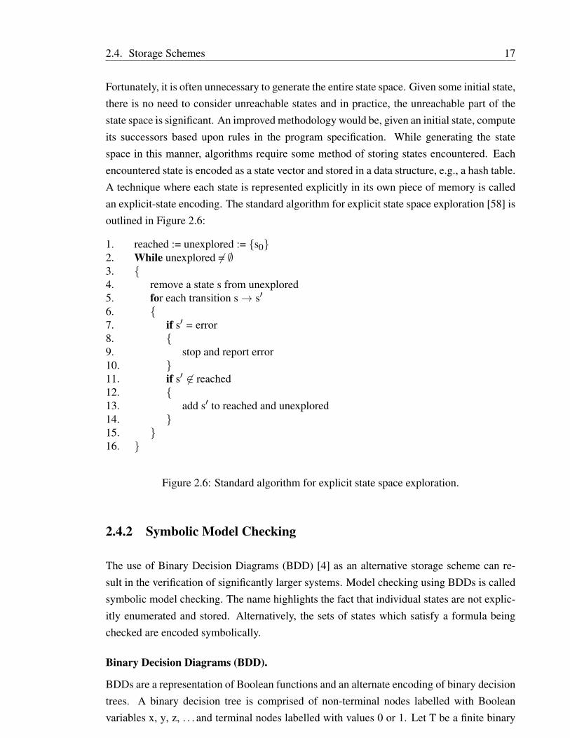
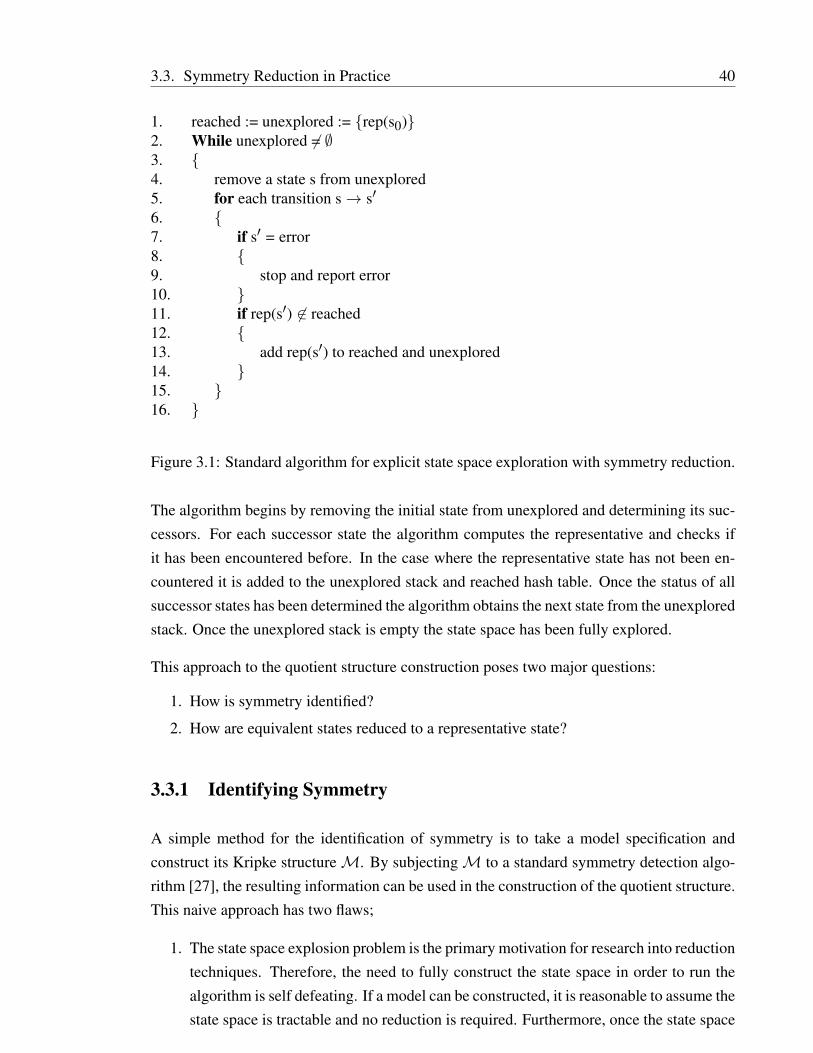
Fortunately, it is often unnecessary to generate the entire state space. Given some initial state,there is no need to consider unreachable states and in practice, the unreachable part of thestate space is significant. An improved methodology would be, given an initial state, computeits successors based upon rules in the program specification. While generating the statespace in this manner, algorithms require some method of storing states encountered. Eachencountered state is encoded as a state vector and stored in a data structure, e.g., a hash table.A technique where each state is represented explicitly in its own piece of memory is calledan explicit-state encoding. The standard algorithm for explicit state space exploration [58] isoutlined in Figure 2.6:
1. reached := unexplored := s02. While unexplored 6= ∅3. 4. remove a state s from unexplored5. for each transition s→ s′6. 7. if s′ = error8. 9. stop and report error10. 11. if s′ 6∈ reached12. 13. add s′ to reached and unexplored14. 15. 16.
Figure 2.6: Standard algorithm for explicit state space exploration.
2.4.2 Symbolic Model Checking
The use of Binary Decision Diagrams (BDD) [4] as an alternative storage scheme can re-sult in the verification of significantly larger systems. Model checking using BDDs is calledsymbolic model checking. The name highlights the fact that individual states are not explic-itly enumerated and stored. Alternatively, the sets of states which satisfy a formula beingchecked are encoded symbolically.
Binary Decision Diagrams (BDD).
BDDs are a representation of Boolean functions and an alternate encoding of binary decisiontrees. A binary decision tree is comprised of non-terminal nodes labelled with Booleanvariables x, y, z, . . . and terminal nodes labelled with values 0 or 1. Let T be a finite binary
2.4. Storage Schemes 18
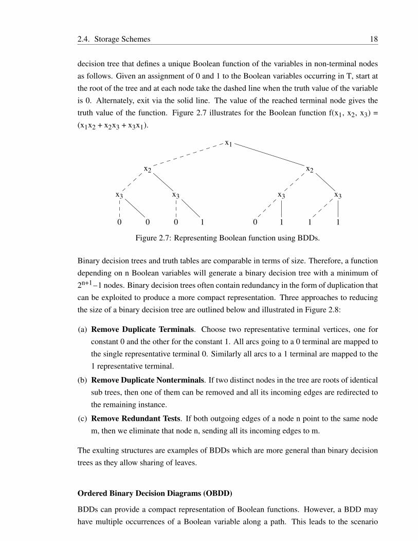
decision tree that defines a unique Boolean function of the variables in non-terminal nodesas follows. Given an assignment of 0 and 1 to the Boolean variables occurring in T, start atthe root of the tree and at each node take the dashed line when the truth value of the variableis 0. Alternately, exit via the solid line. The value of the reached terminal node gives thetruth value of the function. Figure 2.7 illustrates for the Boolean function f(x1, x2, x3) =(x1x2 + x2x3 + x3x1).
x1
x2 x2
x3 x3 x3 x3
0 0 0 1 0 1 1 1
Figure 2.7: Representing Boolean function using BDDs.
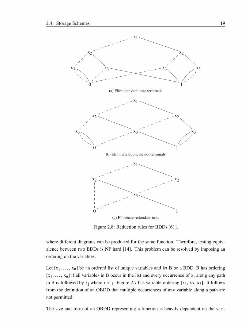
Binary decision trees and truth tables are comparable in terms of size. Therefore, a functiondepending on n Boolean variables will generate a binary decision tree with a minimum of2n+1–1 nodes. Binary decision trees often contain redundancy in the form of duplication thatcan be exploited to produce a more compact representation. Three approaches to reducingthe size of a binary decision tree are outlined below and illustrated in Figure 2.8:
(a) Remove Duplicate Terminals. Choose two representative terminal vertices, one forconstant 0 and the other for the constant 1. All arcs going to a 0 terminal are mapped tothe single representative terminal 0. Similarly all arcs to a 1 terminal are mapped to the1 representative terminal.
(b) Remove Duplicate Nonterminals. If two distinct nodes in the tree are roots of identicalsub trees, then one of them can be removed and all its incoming edges are redirected tothe remaining instance.
(c) Remove Redundant Tests. If both outgoing edges of a node n point to the same nodem, then we eliminate that node n, sending all its incoming edges to m.
The exulting structures are examples of BDDs which are more general than binary decisiontrees as they allow sharing of leaves.
Ordered Binary Decision Diagrams (OBDD)
BDDs can provide a compact representation of Boolean functions. However, a BDD mayhave multiple occurrences of a Boolean variable along a path. This leads to the scenario
2.4. Storage Schemes 19
x1
x2 x2
x3 x3 x3 x3
0 1(a) Eliminate duplicate terminals
x1
x2 x2
x3 x3 x3
0 1(b) Eliminate duplicate nonterminals
x1
x2 x2
x3
0 1(c) Eliminate redundant tests
Figure 2.8: Reduction rules for BDDs [61].
where different diagrams can be produced for the same function. Therefore, testing equiv-alence between two BDDs is NP hard [14]. This problem can be resolved by imposing anordering on the variables.
Let [x1, . . . , xn] be an ordered list of unique variables and let B be a BDD. B has ordering[x1, . . . , xn] if all variables in B occur in the list and every occurrence of xi along any pathin B is followed by xj where i < j. Figure 2.7 has variable ordering [x1, x2, x3]. It followsfrom the definition of an OBDD that multiple occurrences of any variable along a path arenot permitted.
The size and form of an OBDD representing a function is heavily dependent on the vari-
2.4. Storage Schemes 20
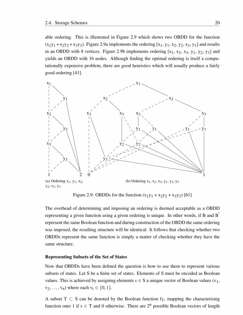
able ordering. This is illustrated in Figure 2.9 which shows two OBDD for the function(x1y1 + x2y2 + x3y3). Figure 2.9a implements the ordering [x1, y1, x2, y2, x3, y3] and resultsin an OBDD with 8 vertices. Figure 2.9b implements ordering [x1, x2, x3, y1, y2, y3] andyields an OBDD with 16 nodes. Although finding the optimal ordering is itself a compu-tationally expensive problem, there are good heuristics which will usually produce a fairlygood ordering [41].
x1
y1
x2
y2
x3
y3
1 2(a) Ordering x1, y1, x2,y2, x3, y3
x1
x2 x2
x3 x3 x3 x3
y1 y1 y1 y1
y2 y2
y3
0 1(b) Ordering x1, x2, x3, y1, y2, y3
Figure 2.9: OBDDs for the function (x1y1 + x2y2 + x3y3) [61]
The overhead of determining and imposing an ordering is deemed acceptable as a OBDDrepresenting a given function using a given ordering is unique. In other words, if B and B
′
represent the same Boolean function and during construction of the OBDD the same orderingwas imposed, the resulting structure will be identical. It follows that checking whether twoOBDDs represent the same function is simply a matter of checking whether they have thesame structure.
Representing Subsets of the Set of States
Now that OBDDs have been defined the question is how to use them to represent varioussubsets of states. Let S be a finite set of states. Elements of S must be encoded as Booleanvalues. This is achieved by assigning elements s ∈ S a unique vector of Boolean values (v1,v2, . . . , vn) where each vi ∈ 0, 1.
A subset T ⊂ S can be denoted by the Boolean function fT, mapping the characterisingfunction onto 1 if s ∈ T and 0 otherwise. There are 2n possible Boolean vectors of length
2.4. Storage Schemes 21
n and so n should be chosen such that 2n – 1 < |S| ≤ 2n, where |S| is the number ofelements in S. For example the set P = (0, 1, 0) (1, 0, 1) has the characteristic functionfP = (¬v1 ∧ v2 ∧ ¬v3) ∨ (v1 ∧ ¬v2 ∧ v3).
When S represents the set of states of a transition system, a subset of atoms can be used toprovide a unique Boolean vector for each s ∈ S. Let P(Atoms) be a set of subsets of Atomswith ordering x1, x2, . . . , xn, state s ∈ S can be represented by the the vector (v1, v2, . . . , vn),where, for each i, vi equals 1 if the atom is valid in the state or 0 otherwise. Consequentlythis state is represented by an OBDD for the Boolean function (l1 · l2 · · · ln) where li is 1if xi is a valid atom and 0 otherwise. The set of states s1, s2, . . . , sm is represented by theOBDD of the Boolean function (l11 · l12 · · · l1n + l21 · l22 · · · l2n + · · · + lm1 · lm2 · · · lmn).
Representing the Transition Relation
A transition relation is defined as R ⊆ S× S. In the section above it was shown that subsetsof a given finite set may be represented as OBDDs by considering the characteristic functionof a binary encoding. To encode a transition relation two copies of a Boolean vector arerequired. Thus, the transition s → t is represented by the pair of Boolean vectors (v1, v2,. . . , vn), (v′1, v′2, . . . , v′n). As an OBDD, the transition is represented by Boolean function (l1· l2 · · · ln) · (l′1 · l′2 · · · l′n) and a set of transitions is the + of such formulae.
The key idea behind applying OBDDs to finite systems is to take a system specification andsynthesise the OBDD directly, without having to go via intermediate representations. For-tunately, certain specification languages enforce updates to variable to be defined using thevariables current value [69, 25]. This type of variable update description can be compiledinto a set of Boolean functions. Therefore, given the OBDD for a set of states and the tran-sition relation, one step successors and one step predecessors can be computed using BDDsymbolic based algorithms. This can be done repeatedly to explore all reachable states [4].
2.4.3 Probabilistic Representations
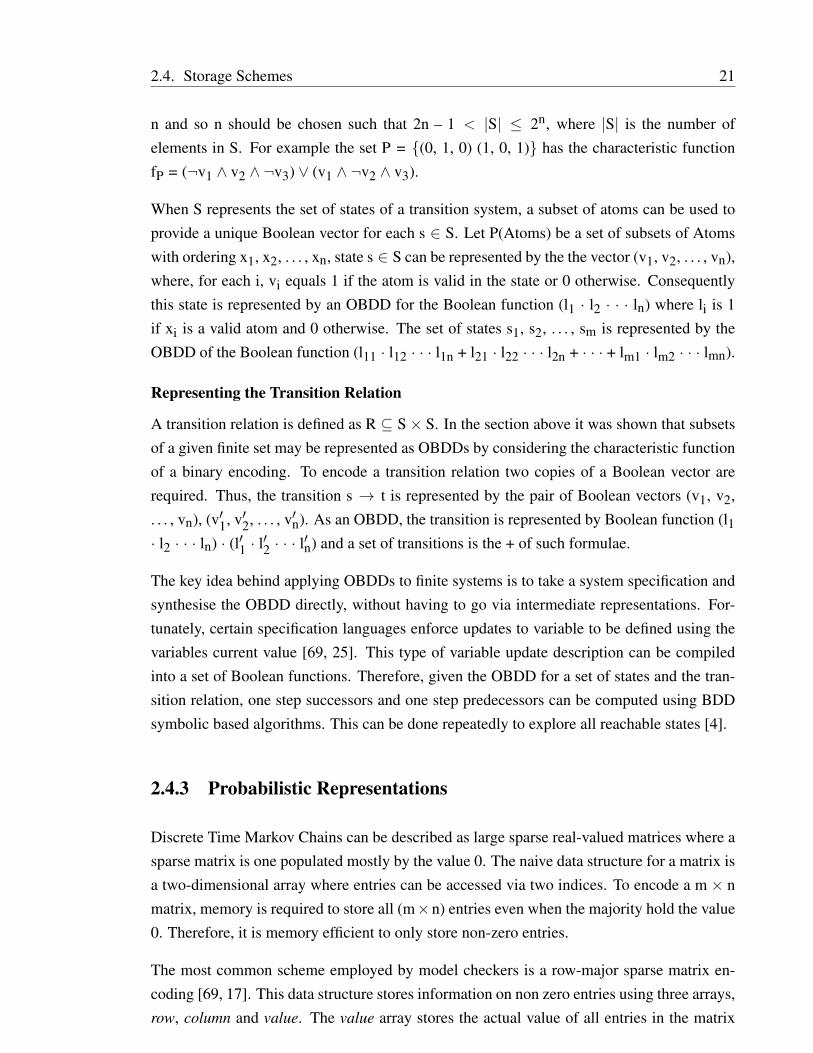
Discrete Time Markov Chains can be described as large sparse real-valued matrices where asparse matrix is one populated mostly by the value 0. The naive data structure for a matrix isa two-dimensional array where entries can be accessed via two indices. To encode a m × nmatrix, memory is required to store all (m×n) entries even when the majority hold the value0. Therefore, it is memory efficient to only store non-zero entries.
The most common scheme employed by model checkers is a row-major sparse matrix en-coding [69, 17]. This data structure stores information on non zero entries using three arrays,row, column and value. The value array stores the actual value of all entries in the matrix
2.4. Storage Schemes 22
while row, stores the column index of each matrix entry. Both these arrays are row ordered.The final array, row, provides a means of indexing into the column array that in turn revealsthe value of a desired element.
For example, an entry in position (r, c) is found by indexing into locations r and r + 1 inrow. The located values are used in turn to index into column positions column[row[r]] andcolumn[row[r+1]–1]. The values contained between and including these indices are checkedto see if they equal c. If the value c is not present, then (r, c) = 0. If it is present, then (r, c) isnon-zero and its value can be found by looking up the value at the same position in the valuearray. An example of this encoding is outlined in Figure 2.10;
· 0.5 · 0.5· · 1 ·
0.3 · · 0.71 · · ·
row 0 2 3 5 6
col 1 3 2 0 3 0val 0.5 0.5 1 0.3 0.7 1
Figure 2.10: A four state DTMC and its sparse storage [82].
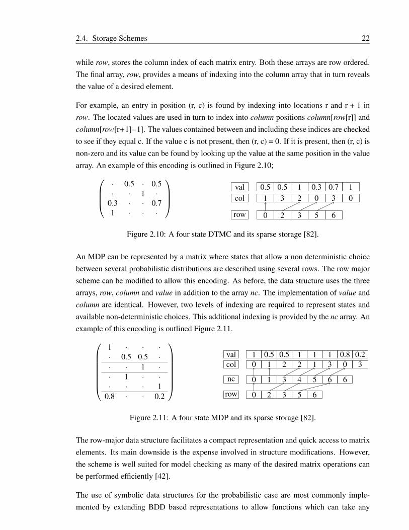
An MDP can be represented by a matrix where states that allow a non deterministic choicebetween several probabilistic distributions are described using several rows. The row majorscheme can be modified to allow this encoding. As before, the data structure uses the threearrays, row, column and value in addition to the array nc. The implementation of value andcolumn are identical. However, two levels of indexing are required to represent states andavailable non-deterministic choices. This additional indexing is provided by the nc array. Anexample of this encoding is outlined Figure 2.11.
1 · · ·· 0.5 0.5 ·· · 1 ·· 1 · ·· · · 1
0.8 · · 0.2
row 0 2 3 5 6
nc 0 1 3 4 5 6 6
col 0 1 2 2 1 3 0 3val 1 0.5 0.5 1 1 1 0.8 0.2
Figure 2.11: A four state MDP and its sparse storage [82].
The row-major data structure facilitates a compact representation and quick access to matrixelements. Its main downside is the expense involved in structure modifications. However,the scheme is well suited for model checking as many of the desired matrix operations canbe performed efficiently [42].
The use of symbolic data structures for the probabilistic case are most commonly imple-mented by extending BDD based representations to allow functions which can take any
2.5. Model Checking Algorithms 23
value, not just 0 or 1. This extension is termed Multiple Terminal Binary Decision Dia-grams MTBDDs and allows a BDD with more than two terminal nodes. Furthermore, ithas been shown that MTBDDs can represent matrices over any finite set as well as imple-menting standard matrix operations, such as scalar multiplication, matrix addition and matrixmultiplication [50].
2.5 Model Checking Algorithms
With the semantic definitions for LTL, CTL and PCTL presented in Section 2.3 and anoverview of representation schemes provided in Section 2.4, we will outline how the rep-resentation schemes can be manipulated to provide answers to posed logical formulae.
2.5.1 CTL Model Checking
The CTL model checking algorithm [22] answers the questionM, s0 |= φ by returning allstates of M that satisfy condition φ. From the returned set of states it is easy to check ifM, s0 |= φ by verifying that the returned set contains s0. The model checking algorithm forCTL is a labelling algorithm that marks states which satisfy sub-formulae of the formula tobe checked. Fortunately, the algorithm does not have to handle every CTL connective as anyformula can be reformulated using only ⊥, ¬ and ∧ and temporal connectives and AF , EUand EX.
The CTL algorithm takes a model M and a CTL formula φ as input. Immediately, φ isreformulated and states of M are labelled with sub formulae of φ that are satisfied in thestate. The algorithm begins with the smallest sub-formulae and works outwards towards φ.Suppose ψ is a sub-formula of φ and states satisfying sub-formulae of ψ have already beenlabelled. The states required to be labelled with ψ can be determined by a case analysis. Ifψ is:
• ⊥: then no states are labelled with ⊥.
• p: where p is an atom from the set of Atoms then label the state with p is true in thestate.
• ψ1 ∧ ψ1 : label s with ψ1 ∧ ψ1 if s is already labelled both with ψ1 and with ψ2 .
• ¬ψ1 : label s with ¬ψ1 if s is not already labelled with ψ1 .
• AF ψ1:– If any state s is labelled with ψ1 , label it with AF ψ1.
2.5. Model Checking Algorithms 24
– Repeat: label any state with AF ψ1 if all successor states are labelled with AF ψ1
, until there is no change.
• E [ψ1 U ψ2 ]:– If any state s is labelled with ψ2 , label it with E [ψ1 U ψ2 ].
– Repeat: label any state with E [ψ1 U ψ2 ] if it is labelled with ψ1 and at least oneof its successors is labelled with E [ψ1 U ψ2 ] , until there is no change.
• EX ψ: label any state with EX ψ if one of its successors is labelled with ψ.
Once all sub-formulae of φ including φ itself have been labelled to states, the set of stateslabelled with φ are returned. The complexity of this algorithm is O(f · V · (V + E)), wheref is the number of formula connectives, V the number of states and E the number of transi-tions [25].
2.5.2 LTL Model Checking
The state-labelling approach of CTL is not appropriate for LTL model checking as sub-formulae are evaluated along paths of a system and not states. While numerous implemen-tations of slightly different LTL model checking algorithm appear in the literature [54, 58],nearly all follow the same strategy [61]. These algorithms take a modelM, a state s ∈ S anda LTL formula φ as input and determine whetherM, s |= φ using the following steps:
1. Construct an automaton for the formula ¬φ, denoted A¬φ. A¬φ accepts a trace that is asequence of valuations of the propositional atoms. Thus, the automaton A¬φ encodesall the traces satisfying the property A¬φ. A trace can be generated for any path.
2. Combine A¬φ and system modelM. This results in a new automaton that has all thepaths of A¬φ andM. In practice the new system is constructed by letting the systemmodelM and the automaton for the formula A¬φ to take alternate progressing steps.
3. Attempt to find a path from the starting state to a set of final states defined by A¬φ.If such a path is found it can be interpreted to mean that M, s 6|= φ. In this instance acounterexample can be extracted from the located path.
The complexity of this algorithm is O(|S| + |R| · 2O(|φ|)) and is therefore exponential in thelength of the formula to be checked [58]. In the worst case this means that LTL model check-ing is significantly more complex than CTL model checking. Fortunately, the worst case israrely achieved and in practice there is little run time difference between the algorithms.
2.5. Model Checking Algorithms 25
2.5.3 PCTL Model Checking
The PCTL model checking algorithm [53] is similar to the CTL model checking algorithmdetailed in Section 2.5.1. However, it is now necessary to compute relevant probabilities.For model checking operator P./prob[ψ] applied to a DTMC the probability of a path leavingeach state s satisfying the path formula ψ must be computed. This may require a calculationinvolving the operators Ps(X φ) , Ps(φ U≤k ψ) and Ps(φ U ψ). With this information it isthen possible to compute Sat(P./prob[ψ] as s ∈ S Ps(ψ) ./ prob.
The Next Operator
Observe that Ps(X φ) is the sum of the probabilities of reaching a state in the next transitionwhere φ holds i.e.
∑s′∈Sat(φ) P(s, s′). Let φ be a vector indexed by states where φ(s) = 1 if
s |= φ and φ(s) = 0 if s 6|= φ. Vector P(X φ) of required probabilities can be calculated by thematrix-vector multiplication P · φ.
The Bounded Until Operator
To perform the calculation associated with this operator the set of states are divided into thethree disjoint sets: Sno = S \ (Sat(φ1) ∪ Sat(φ2)), Syes = Sat(φ2) and S? = S \ (Sno ∪ Syes).The sets Syes and Sno contain the states where Ps(φU≤kφ) equals 1 and 0 respectively andS? contains all other states. For the set of states S?, we have
Ps(φ1U≤kφ2) =
0 if k = 0∑
s′∈S P(s, s′) · Ps(φ1U≤k–1φ2) if k ≥ 1
Let Ps(φ U≤k φ) be a state indexed vector and by defining the matrix P′ as follows
P′(s, s′) =
P′(s, s′) if ∈ S?
1 if s ∈ Syes and s = s′
0 if s ∈ Sno
the required probabilities can be computed in the following manner. If k = 0 and s ∈ Syes,P0(s) = 1 and if s ∈ Sno, P0(s) = 0. In the instance where k ≥ 1 vector Ps(φ1U≤k–1 φ2) canbe calculated by k matrix-vector multiplication P′· Ps(φ1U≤k–1 φ2).
The Until Operator
As with the bounded until operator, all states are divided into the three disjoint sets, Syes,Sno and S?. The sets are defined as above, however sets Syes, Sno are extended to contain all
2.5. Model Checking Algorithms 26
states for which Ps(φ1 U φ2) are respectively, 1 or 0. Set Sno is calculated by first computingthe set of states reachable with non-zero probability satisfying φ2 whose predecessors donot satisfying φ1. Subtracting these states from set S, produces the set of states with 0probability. Set Syes similarly calculates the set of states reachable with probability less than1, that satisfy φ2 whose predecessors do not satisfy φ1. By subtracting these states from S,the set of states satisfying the operator with probability 1 is determined.
The reason behind the pre-computation of Syes, Sno is that it ensures a unique solution to thelinear equation system and reduces the set of states in S?, for which probabilities must becomputed numerically. Furthermore, the model checking of qualitative properties where theprobability bound is 1 or 0 requires no further computation. The final set S? can be calculatedby solving the linear equation
Ps(φ1Uφ2) =
∑
s′∈S P(s, s′) · Ps(φ1Uφ2) if s ∈ S?
1 if s ∈ Syes
0 if s ∈ Sno
To reconstruct the problem in the form Ax = b. Let b be the state indexed vector whereb(s) = 1 if s ∈ Syes and b(s) = 0 if s ∈ Sno, and A = I – P′ where I is the the identity matrixand matrix P′ is as defined below;
P′(s, s′) =
P(s, s′) if s ∈ S?
0 if s ∈ Syes
0 if s ∈ Sno
The linear equation system Ax = b can then be solved using direct methods, such as Gaussianelimination, or iterative methods, such as Jacobi, Gauss-Seidel or the Power method [93].In model checking it is common to have to manage large models and therefore iterativemethods are preferred. Gauss-Seidel typically outperforms Jacobi due to faster convergenceand has the added benefit of only needing to store a single solution vector. Both of thesemethods usually outperform the Power method. However the Power method has guaranteedconvergence.
PCTL model checking over MDPs
For an MDP computing the probabilities of the PCTL operators: next, bounded until anduntil differs as all adversaries A∈ Adv have to be accounted for. To determine if a probabilitybound holds either the maximum or minimum probability for the PCTL formula is calculateddepending whether the relational operator defines an upper or lower bound. Furthermore, the
2.5. Model Checking Algorithms 27
calculation method for maximum and minimum probabilities changes depending whetherthe set of all adversaries or just the set of fair adversaries is considered. In practice thisconsideration only affects the until operator as fairness only places restrictions on the long-run behaviour of the system.
The Next Operator
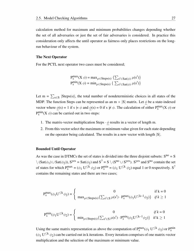
For the PCTL next operator two cases must be considered;
Pmaxs (X φ) = maxµ∈Steps(s)
∑s′∈Sat(φ) µ(s′)
Pmins (X φ) = minµ∈Steps(s)
∑s′∈Sat(φ) µ(s′)
Let m =∑
s∈S |Steps(s)|, the total number of nondeterministic choices in all states of theMDP. The function Steps can be represented as an m× |S| matrix. Let φ be a state-indexedvector where φ(s) = 1 if s |= φ and φ(s) = 0 if s 6|= φ. The calculation of either Pmax
s (X φ) orPmin
s (X φ) can be carried out in two steps:
1. The matrix-vector multiplication Steps · φ results in a vector of length m.
2. From this vector select the maximum or minimum value given for each state dependingon the operator being calculated. The results in a new vector with length |S|.
Bounded Until Operator
As was the case in DTMCs the set of states is divided into the three disjoint subsets: Sno = S\ (Sat(φ1)∪ Sat(φ2)), Syes = Sat(φ2) and S? = S \ (Sno ∪ Syes). Syes and Sno contain the setof states for which Pmax
s = (φ1 U≤k φ2) or Pmins = (φ1 U≤k φ2) equal 1 or 0 respectively. S?
contains the remaining states and there are two cases;
Pmaxs (φ1U≤kφ2) =
0 if k = 0
maxµ∈Steps(s)∑
s′∈S µ(s′) · Pmaxs (φ1U≤k–1φ2) if k ≥ 1
Pmins (φ1U≤kφ2) =
0 if k = 0
minµ∈Steps(s)∑
s′∈S µ(s′) · Pmins (φ1U≤k–1φ2) if k ≥ 1
Using the same matrix representation as above the computation of Pmaxs (φ1 U≤k φ2) or Pmin
s(φ1 U≤k φ2) can be carried out in k iterations. Every iteration comprises of one matrix-vectormultiplication and the selection of the maximum or minimum value.
2.5. Model Checking Algorithms 28
The Until Operator
For the PCTL operator until we must compute either Pmaxs = Pmax
s (φ1 U φ2) or Pmins =
Pmins (φ1 U φ2). Two cases must be considered, all adversaries and fair adversaries. For
clarity PAs will be used to denote PA
s (φ1 U φ2). Beginning with the case for the set of alladversaries the set of states are divided into the three disjoint subsets Sno = S \ (Sat(φ1) ∪Sat(φ2)), Syes = Sat(φ2) and S? = S \ (Sno ∪ Syes).
For Pmaxs , Sno contains the set of states for which PA
s = 0 for every adversary A. The calcula-tion of Pmax
s proceeds by first computing the set of states reachable with non-zero probabilityunder some adversary that satisfy φ2 and whose predecessors satisfied φ1. Removing thesestates from set S produces the set of states with probability 0. For Pmin
s , Sno contains allstates for which PA
s = 0 for some adversary A and is computed in a similar fashion.
The algorithm for the computation of Pmaxs in the set Syes is more complex but works on the
same principle of calculating the states reachable with probability less than 1 and subtractingfrom set S. The algorithm depends on two nested loops .The outer loop computes a set ofstates R and by the end of its execution will contain all states where PA
s = 1 for someadversary A. With each iteration of the outer loop, invalid states that were identified by theinner loop are removed. They are determined as the states which can no longer reach a statewhere Sat(φ2) without passing through a state not in Sat(φ1) or a previously removed state.For pmin
s , Sno is assumed to be the set of states Sat(φ2) for which Pmins is trivially 1.
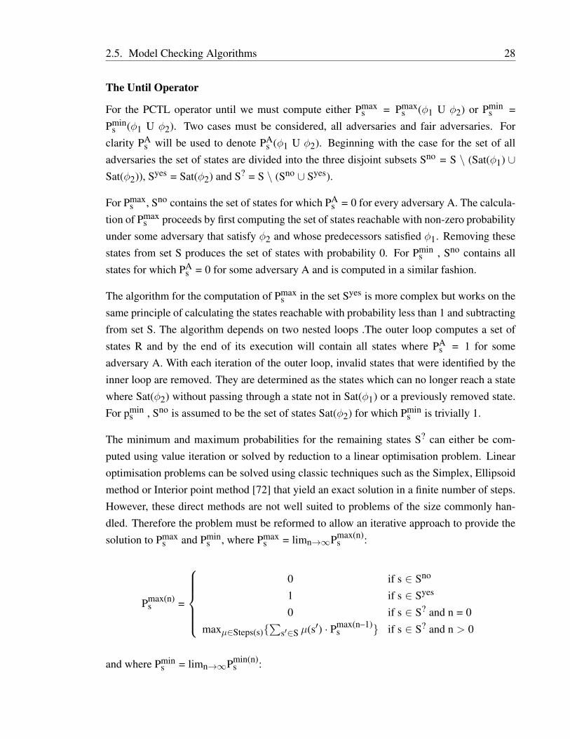
The minimum and maximum probabilities for the remaining states S? can either be com-puted using value iteration or solved by reduction to a linear optimisation problem. Linearoptimisation problems can be solved using classic techniques such as the Simplex, Ellipsoidmethod or Interior point method [72] that yield an exact solution in a finite number of steps.However, these direct methods are not well suited to problems of the size commonly han-dled. Therefore the problem must be reformed to allow an iterative approach to provide thesolution to Pmax
s and Pmins , where Pmax
s = limn→∞Pmax(n)s :
Pmax(n)s =
0 if s ∈ Sno
1 if s ∈ Syes
0 if s ∈ S? and n = 0
maxµ∈Steps(s)∑
s′∈S µ(s′) · Pmax(n–1)s if s ∈ S? and n > 0
and where Pmins = limn→∞Pmin(n)
s :
2.6. Model Checking Tools 29
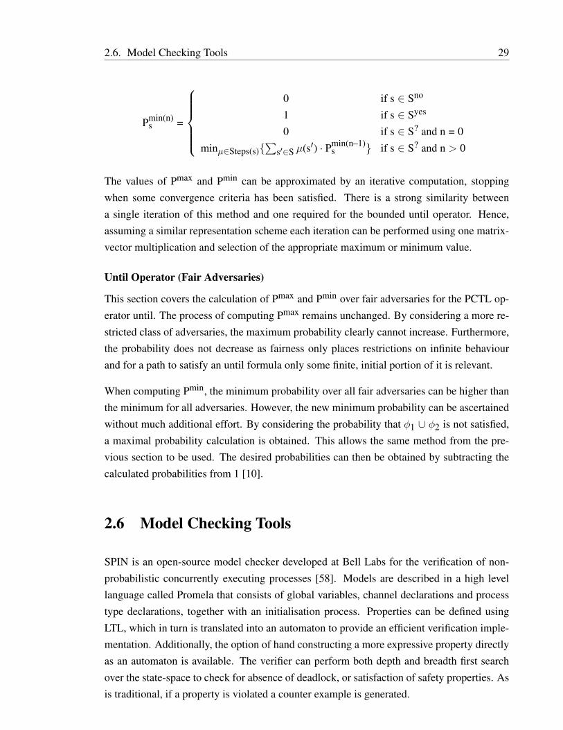
Pmin(n)s =
0 if s ∈ Sno
1 if s ∈ Syes
0 if s ∈ S? and n = 0
minµ∈Steps(s)∑
s′∈S µ(s′) · Pmin(n–1)s if s ∈ S? and n > 0
The values of Pmax and Pmin can be approximated by an iterative computation, stoppingwhen some convergence criteria has been satisfied. There is a strong similarity betweena single iteration of this method and one required for the bounded until operator. Hence,assuming a similar representation scheme each iteration can be performed using one matrix-vector multiplication and selection of the appropriate maximum or minimum value.
Until Operator (Fair Adversaries)
This section covers the calculation of Pmax and Pmin over fair adversaries for the PCTL op-erator until. The process of computing Pmax remains unchanged. By considering a more re-stricted class of adversaries, the maximum probability clearly cannot increase. Furthermore,the probability does not decrease as fairness only places restrictions on infinite behaviourand for a path to satisfy an until formula only some finite, initial portion of it is relevant.
When computing Pmin, the minimum probability over all fair adversaries can be higher thanthe minimum for all adversaries. However, the new minimum probability can be ascertainedwithout much additional effort. By considering the probability that φ1 ∪ φ2 is not satisfied,a maximal probability calculation is obtained. This allows the same method from the pre-vious section to be used. The desired probabilities can then be obtained by subtracting thecalculated probabilities from 1 [10].
2.6 Model Checking Tools
SPIN is an open-source model checker developed at Bell Labs for the verification of non-probabilistic concurrently executing processes [58]. Models are described in a high levellanguage called Promela that consists of global variables, channel declarations and processtype declarations, together with an initialisation process. Properties can be defined usingLTL, which in turn is translated into an automaton to provide an efficient verification imple-mentation. Additionally, the option of hand constructing a more expressive property directlyas an automaton is available. The verifier can perform both depth and breadth first searchover the state-space to check for absence of deadlock, or satisfaction of safety properties. Asis traditional, if a property is violated a counter example is generated.
2.6. Model Checking Tools 30
The combination of the Promela language and SPIN verifier has been widely used in safetycritical systems. Examples including the verification of control algorithms for a movablestorm surge barrier where manual management was considered too high a risk [92]. A morerecent example is verification of the resource arbiter used to manage all motors on the MarsExploration Rovers [59].
Another example of an explicit-state model checker is Murφ [29]. The Murφ specificationlanguage consists of infinitely executing guarded commands and unlike SPIN there is noprovision for temporal logics. The verifier can only check the state-space for absence ofdeadlock, or satisfaction of assert statements. Murφ has seen most use in the design of cachecoherence algorithms and protocols.
For non-probabilistic symbolic model checkers Symbolic Model Verifier, SMV is the bench-mark implementation [25]. SMV uses an OBDD based algorithm for the verification of CTLproperties against a specification written in the SMV language. The SMV language supportsfinite data structures such as Booleans, scalars and fixed arrays. The primary purpose of thelanguage is the specification of the transition relation which in turn allows the generationof the OBDD directly from the language description. Perhaps the most recognised appli-cation of SMV is in the verification of the Cache Coherence Protocols for Distributed FileSystems [25].
In the probabilistic realm a tool for Qualitative and Quantitative Linear Time analysis ofReactive Systems, LiQuor [17], was developed by the University of Bonn. LiQuor is a toolfor verifying probabilistic reactive systems specified in ProbMela, a probabilistic guardedcommand language inspired by the modelling language Promela [8]. Like SPIN, LiQuorrelies on the automata-based approach to model check linear time properties. The underlyingdata structure is explicit in nature and is used to encode an MDP. In design, LiQuor is anamalgamation of many separate tools, the ProbMela compiler, Cocktail providing the userinterface and Appetizer for user driven simulation.
The Markov Reward Model Checker [64] provides model checking of CSL over CTMCsand PCTL over DTMCs. Both Markov Chains are stored in explicit data structures such assparse matrices. The transition matrices for the DTMCs or CTMCs to be analysed are alsospecified explicitly: the user provides a list of all the states and transitions which make upthe model. The format in which checker accepts information allows it to be easily integratedwith other tools.
Finally, the Probabilistic Symbolic Model Checker, PRISM [69], was developed at the Uni-versity of Birmingham. It is a probabilistic model checker that employs automatic formalverification techniques to enable the analysis of stochastic systems. PRISM provides support
2.6. Model Checking Tools 31
for three types of probabilistic models; DTMCs, MDPs and CTMCs. The basic underlyingdata structures of PRISM are BDDs and MTBDDs. However, PRISM provides three distinctengines. The first is a pure MTBDD implementation, the second is explicit, based on sparsematrices; and the third uses a hybrid symbolic, explicit approach. Properties of models arewritten in the PRISM property specification language, based on the three probabilistic tem-poral logics PCTL and LTL for DTMCs, PCTL for MDPs, and CSL for CTMCs. Further,analytical abilities include the power to enhance the richness of models, by the assignmentof costs and rewards to certain model behaviours, i.e transitions within the model. PRISMalso provides wide ranging support for the automated analysis of quantitative properties.
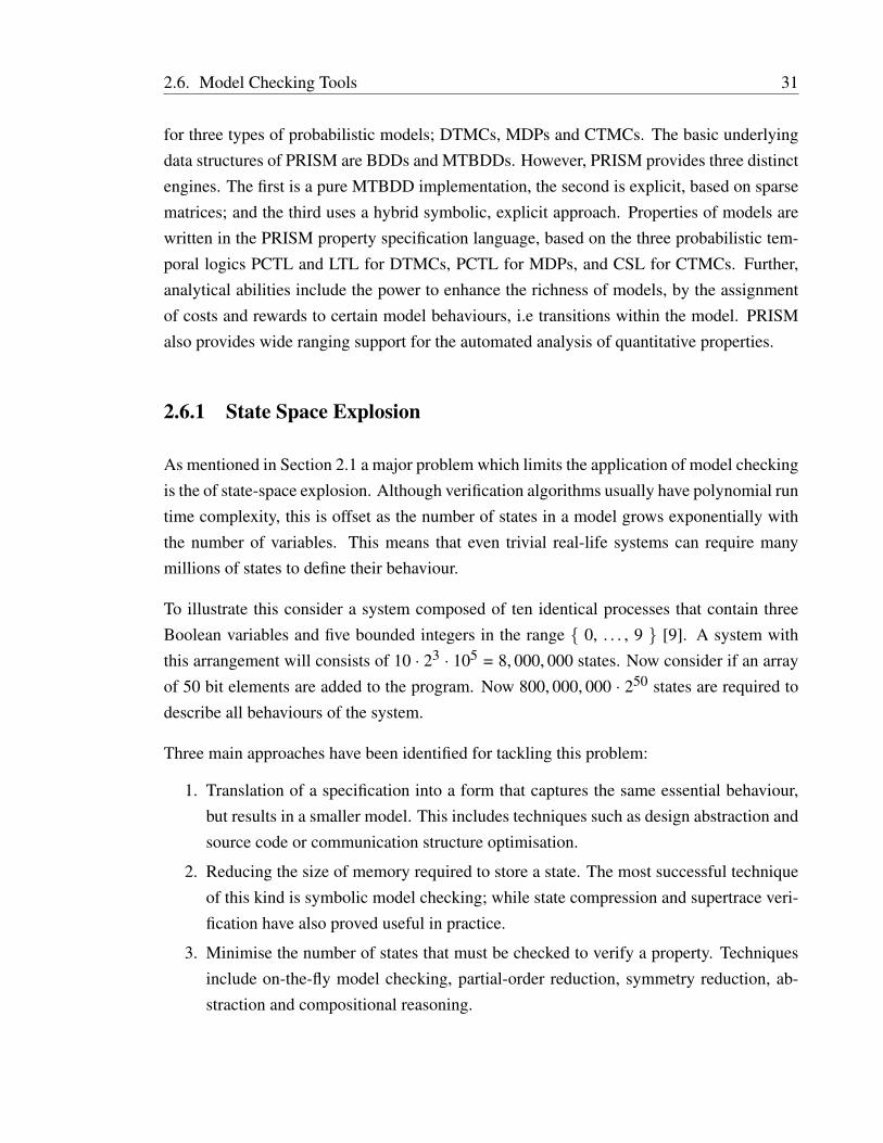
2.6.1 State Space Explosion
As mentioned in Section 2.1 a major problem which limits the application of model checkingis the of state-space explosion. Although verification algorithms usually have polynomial runtime complexity, this is offset as the number of states in a model grows exponentially withthe number of variables. This means that even trivial real-life systems can require manymillions of states to define their behaviour.
To illustrate this consider a system composed of ten identical processes that contain threeBoolean variables and five bounded integers in the range 0, . . . , 9 [9]. A system withthis arrangement will consists of 10 · 23 · 105 = 8, 000, 000 states. Now consider if an arrayof 50 bit elements are added to the program. Now 800, 000, 000 · 250 states are required todescribe all behaviours of the system.
Three main approaches have been identified for tackling this problem:
1. Translation of a specification into a form that captures the same essential behaviour,but results in a smaller model. This includes techniques such as design abstraction andsource code or communication structure optimisation.
2. Reducing the size of memory required to store a state. The most successful techniqueof this kind is symbolic model checking; while state compression and supertrace veri-fication have also proved useful in practice.
3. Minimise the number of states that must be checked to verify a property. Techniquesinclude on-the-fly model checking, partial-order reduction, symmetry reduction, ab-straction and compositional reasoning.
2.7. Summary 32
2.7 Summary
In this chapter we have provided a detailed account of current approaches to model check-ing, starting with theory and working through to implementation. The chapter closes bymentioning the state space explosion problem and the wide variety of techniques that havebeen proposed to combat it. In the next chapter we will specifically focus on the state spacemanagement technique of symmetry reduction.
CHAPTER 3
Symmetry Reduction
This chapter presents established approaches for the state space management technique ofSymmetry Reduction. Section 3.1 introduces the notion of Symmetry Reduction with Sec-tion 3.2 providing a mathematical explanation for its application in the context of modelchecking. Issues concerning the identification and application of symmetry are discussedin Section 3.3 and Section 3.4 respectively. The chapter closes with a review of currentlyavailable tools that implement an approach to symmetry reduction.
Concurrent systems often contain replication and as a result model checking algorithms mayspend a significant proportion of time searching over equivalent areas of the state space.Consider a system comprised of numerous processes running the same program. The onlydistinguishable difference between them is the process name. In this instance processes canbe viewed as interchangeable and any transformation that consistently swaps them through-out the system will not impact the overall set of system behaviours. Once a symmetry hasbeen established the question becomes how to exploit the knowledge during verification.
Continuing the example, every system state does not have to be individually encountered andstored, they can be collapsed into one representative state in a reduced system. Therefore,given n processes, potentially n! original states can be collapsed and their behaviours rep-resented by a single new state in a reduced system. Consider the mutual exclusion protocoloutlined in Figure 2.3. This example consists of 2 identical processes, excluding processidentifiers, and clearly demonstrates the existence of symmetry within a Kripke structure.
33
3.1. Group Theory 34
Furthermore, the mutual exclusion property AG (¬(C1 ∧ C2)) holds for any state A, B andB, A, where A and B take a value from the set N, T, C. If state A, B satisfies the mutualexclusion property so does B, A.
3.1 Group Theory
Symmetries of a model structure form a group and the survey of symmetry reduction tech-niques in this chapter, and the techniques develop throughout the thesis require some def-initions and results from group theory. This section covers basic definitions [73, 56] andprovides a specific overview of Permutation and Symmetric Groups.
3.1.1 Groups, Subgroups and Homomorphisms
Definition. A group (G, ∗) contains a set S with a closed binary operation ∗ such that thegroup axioms hold;
1. For every x, y, z ∈ G, we have (x ∗ y) ∗ z = x ∗ (y ∗ z).
2. There is an element e ∈ G such that for every x ∈ G, e ∗ x = x ∗ e = x.
3. For each x ∈ G there is an element x′ ∈ G such that x ∗ x′ = x′ ∗ x = e.
The number of distinct elements in a finite group G, is called the order of the group and isdenoted by |G|. The identity element is denoted by e or eG if ambiguous, and the inverse ofan element x of G is denoted by x–1 . Finally, the binary operation ∗, usually a compositionof mappings is written xy for x ∗ y.
Definition. A group is called abelian or commutative if it satisfies the additional property,x ∗ y = y ∗ x for all elements xy ∈ G.
Definition. A subset H of a group G is called a subgroup of G if the following conditionsare satisfied:
1. eG ∈ H.
2. if x, y ∈ H then xy ∈ H.
3. if x ∈ H, then x–1 ∈ H.
If H is a subgroup of G it can be written H ≤ G. Additionally, a subgroup H is propersubgroup if H 6= G and is written H < G.
3.1. Group Theory 35
Definition. Let H be a subgroup of G and g ∈ G then the subset gH = gh | h ∈ H ⊆ G iscalled the left coset of H. Similarly the subset Hg = hg | h ∈ H ⊆ G is the right coset ofH. The set of left cosets of H is denoted G/H and the set of right cosets H\G.
Definition. Let A be any subset of a group G. The subgroup of G generated by A, denoted〈A〉, or 〈x1, x2 . . . , xn 〉 if A = x1, x2, . . . , xn is the intersection of all subgroups of Gcontaining A.
The group 〈A〉 is the smallest subgroup of G that contains A. It is often the case in compu-tational applications that the generating set x1, x2, . . . , xn has an ordering that is definedimplicitly by the subscript of xi
Definition. Let (G, ∗) and (H, ) be groups. A function f : G→ H is a homomorphism if forall a, b ∈ G ,
f(a ∗ b) = f(a) f(b)
A homomorphism σ is called a monomorphism, epimorphism or isomorphism if it is aninjection, surjection or bijection, respectively. Groups G and H are isomorphic if there is anisomorphism σ : G→ H, denoted G ∼= H. Finally an isomorphism from group G onto itselfis called an automorphism.
3.1.2 Permutation Group
Definition. If X is a non empty set, a permutation of X is a bijection α : X → X The set ofall permutations of X is denoted SX
Let X be a set. The symmetric group, Sym(X), consists of all the bijections from X to X,with map compositions as the group operator. A recurring special case is where X is finite,consisting of the first n natural numbers. Under these conditions the symmetric group istermed Sn.
Any bijection α can be denoted by two rows;
α =
(1 2 . . . nα1 α2 . . . αn
),
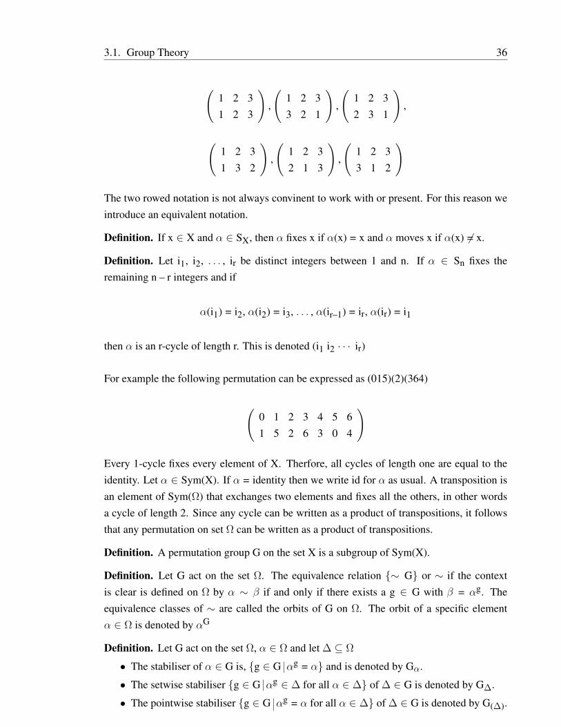
and the bottom row is a rearrangment of 1, 2, . . . , n. If Γ is a set of size n, then thereis a bijection θ : Γ → 1, 2, . . . , n which induces a mapping θ : Sym(Γ) → Sn via(σ)θ = θ–1 σ θ for every σ ∈ Sym(Γ). For example the Symmetric group S3 is;
3.1. Group Theory 36
(1 2 31 2 3
),
(1 2 33 2 1
),
(1 2 32 3 1
),
(1 2 31 3 2
),
(1 2 32 1 3
),
(1 2 33 1 2
)
The two rowed notation is not always convinent to work with or present. For this reason weintroduce an equivalent notation.
Definition. If x ∈ X and α ∈ SX, then α fixes x if α(x) = x and α moves x if α(x) 6= x.
Definition. Let i1, i2, . . . , ir be distinct integers between 1 and n. If α ∈ Sn fixes theremaining n – r integers and if
then α is an r-cycle of length r. This is denoted (i1 i2 · · · ir)
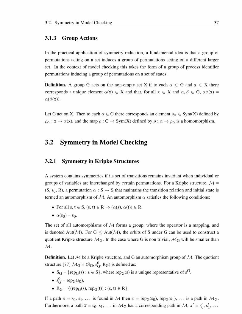
For example the following permutation can be expressed as (015)(2)(364)
(0 1 2 3 4 5 61 5 2 6 3 0 4
)
Every 1-cycle fixes every element of X. Therfore, all cycles of length one are equal to theidentity. Let α ∈ Sym(X). If α = identity then we write id for α as usual. A transposition isan element of Sym(Ω) that exchanges two elements and fixes all the others, in other wordsa cycle of length 2. Since any cycle can be written as a product of transpositions, it followsthat any permutation on set Ω can be written as a product of transpositions.
Definition. A permutation group G on the set X is a subgroup of Sym(X).
Definition. Let G act on the set Ω. The equivalence relation ∼ G or ∼ if the contextis clear is defined on Ω by α ∼ β if and only if there exists a g ∈ G with β = αg. Theequivalence classes of ∼ are called the orbits of G on Ω. The orbit of a specific elementα ∈ Ω is denoted by αG
Definition. Let G act on the set Ω, α ∈ Ω and let ∆ ⊆ Ω
• The stabiliser of α ∈ G is, g ∈ G αg = α and is denoted by Gα.
• The setwise stabiliser g ∈ G αg ∈ ∆ for all α ∈ ∆ of ∆ ∈ G is denoted by G∆.
• The pointwise stabiliser g ∈ G αg = α for all α ∈ ∆ of ∆ ∈ G is denoted by G(∆).
3.2. Symmetry in Model Checking 37
3.1.3 Group Actions
In the practical application of symmetry reduction, a fundamental idea is that a group ofpermutations acting on a set induces a group of permutations acting on a different largerset. In the context of model checking this takes the form of a group of process identifierpermutations inducing a group of permutations on a set of states.
Definition. A group G acts on the non-empty set X if to each α ∈ G and x ∈ X therecorresponds a unique element α(x) ∈ X and that, for all x ∈ X and α, β ∈ G, αβ(x) =α(β(x)).
Let G act on X. Then to each α ∈ G there corresponds an element ρα ∈ Sym(X) defined byρα : x→ α(x), and the map ρ : G→ Sym(X) defined by ρ : α→ ρα is a homomorphism.
3.2 Symmetry in Model Checking
3.2.1 Symmetry in Kripke Structures
A system contains symmetries if its set of transitions remains invariant when individual orgroups of variables are interchanged by certain permutations. For a Kripke structure,M =(S, s0, R), a permutation α : S → S that maintains the transition relation and initial state istermed an automorphism ofM. An automorphism α satisfies the following conditions:
• For all s, t ∈ S, (s, t) ∈ R⇒ (α(s), α(t)) ∈ R.
• α(s0) = s0.
The set of all automorphisms of M forms a group, where the operator is a mapping, andis denoted Aut(M). For G ≤ Aut(M), the orbits of S under G can be used to construct aquotient Kripke structureMG. In the case where G is non trivial,MG will be smaller thanM.
Definition. LetM be a Kripke structure, and G an automorphism group ofM. The quotientstructure [77]MG = (SG, s0
G, RG) is defined as:
• SG = repG(s) : s ∈ S, where repG(s) is a unique representative of sG.
• s0G = repG(s0).
• RG = (repG(s), repG(t)) : (s, t) ∈ R.
If a path π = s0, s1, . . . is found inM then π = repG(s0), repG(s1), . . . is a path inMG.Furthermore, a path π = s0, s1, . . . inMG has a corresponding path inM, π′ = s′0, s′1, . . .
3.2. Symmetry in Model Checking 38
such that s′0 = s0 and for all i ≥ 1, s′i ∈ sGi . Proofs of these statements have been presented
and show a bidirectional correspondence between paths ofM and the quotient structureMG
for any group of automorphisms G ofM [77].
Therefore, for a modelM and its quotient model MG with respect to a group G, M, s |=φ⇔MG, repG(s) |= φ for every symmetric CTL? formula. A CTL? formula φ is symmetricif for each propositional subformula f, and for all α ∈ G, s |= f ⇔ α(s) |= f. It follows thatM |= φ⇔MG |= φ.
3.2.2 Symmetry in Discrete Time Markov Chains
For a DTMC, D = (S, s0, P), a permutation α : S → S that maintains the transition proba-bilities and initial state is termed an automorphism of D. An automorphism α satisfies thefollowing conditions:
• For all s, t ∈ S, P(s, t) = P(α(s), α(t)).
• α(s0) = s0.
The set of all automorphisms of D forms a group where the operator is a mapping and isdenoted Aut(D). For G ≤ Aut(D), the orbits of S under G can be used to construct aquotient DTMC DG
Definition. Let D be a DTMC, and G be an automorphism group of D. The quotient struc-ture [77] DG = (SG, s0
G, PG) is defined as:
• SG = repG(s) : s ∈ S, where repG(s) is a unique representative of sG.
• s0G = repG(s0).
• PG(repG(s), repG(t)) =∑
x∈tG P(repG(s), x).
If a path π = s0, s1, . . . is found in D then π = repG(s0), repG(s1), . . . is a path in DG.Furthermore, a path π = s0, s1, . . . in DG has a corresponding path in D, π′ = s′0, s′1, . . .such that s′0 = s0 and for all i ≥ 1, s′i ∈ sG
i . Proofs of these statements have been presentedand show a bidirectional correspondence between paths of D and the quotient structure DG
for any group of automorphisms G of D [77].
Therefore for a model D and its quotient model DG with respect to a group G, D, s |= φ ⇔DG, repG(s) |= φ for every symmetric PCTL formula. A PCTL formula φ is symmetric iffor each propositional subformula f, and for all α ∈ G, s |= f ⇔ α(s) |= f. It follows thatD |= φ⇔ DG |= φ.
3.3. Symmetry Reduction in Practice 39
3.2.3 Symmetry in Markov Decision Process
For an MDP,M = (S, s0, Steps), a permutation α : S→ S that maintains the transition prob-abilities and initial states is termed an automorphism of M. An automorphism α satisfiesthe following conditions:
• For all s, t ∈ S for which there exists a µ ∈ Steps and µ(t) > 0, there exists µ′ ∈(Steps(α(s))) such that µ′(α(t)) = µ(t).
• α(s0) = s0.
The set of all automorphisms ofM forms a group where the operator is a mapping and isdenoted Aut(M). For G ≤ Aut(M), the orbits of S under G can be used to construct aquotient MDPMG.
Definition. LetM be a MDP, and G be an automorphism group ofM. The quotient struc-ture [77]MG = (SG, s0
G, StepsG) is defined as:
• SG = repG(s) : s ∈ S, where repG(s) is a unique representative of sG .
• S0G = repG(s0).
• for each repG(s) ∈ SG and µ ∈ Steps(repG(s)), StepsG(repG(s)) contains a distributionµ ∈ Dist(SG) where, for repG(t) ∈ SG, µ(repG(t)) =
∑x∈tG µ(x).
If a path π = s0µ1–––→ s1,
µ2–––→ . . . is found inM then π = repG(s0)µ1–––→ repG(s1)
µ2–––→ . . . is
a path inMG. Furthermore, a path π = s0µ1–––→ s1
µ2–––→ . . . has a corresponding path inM,
π′ = s′0µ′1–––→ s′1
µ′2–––→ . . . such that s′0 = s0, s′i ∈ sGi . Proofs of these statements have been
presented and show a bidirectional correspondence between paths of M and the quotientstructureMG for any group of automorphisms G ofM [77].
Therefore for a modelM and its quotient modelMG with respect to a group G, M, s |= φ⇔MG, repG(s) |= φ for every symmetric PCTL formula. It follows thatM |= φ⇔ MG |= φ.
3.3 Symmetry Reduction in Practice
The key idea of symmetry reduction is to exploit the underlying structure of the transitionsystem in an attempt to reduce the size of the state space. The state space exploration al-gorithm, outlined in Figure 2.6, can be adapted to exploit equivalence between states. Theadapted algorithm, presented in Figure 3.1, allows a quotient state space to be incremen-tally constructed if symmetries are known in advance. The major benefit of this approach isthat the quotient structure may be built even though the original structure is too large to beexplored.
3.3. Symmetry Reduction in Practice 40
1. reached := unexplored := rep(s0)2. While unexplored 6= ∅3. 4. remove a state s from unexplored5. for each transition s→ s′6. 7. if s′ = error8. 9. stop and report error10. 11. if rep(s′) 6∈ reached12. 13. add rep(s′) to reached and unexplored14. 15. 16.
Figure 3.1: Standard algorithm for explicit state space exploration with symmetry reduction.
The algorithm begins by removing the initial state from unexplored and determining its suc-cessors. For each successor state the algorithm computes the representative and checks ifit has been encountered before. In the case where the representative state has not been en-countered it is added to the unexplored stack and reached hash table. Once the status of allsuccessor states has been determined the algorithm obtains the next state from the unexploredstack. Once the unexplored stack is empty the state space has been fully explored.
This approach to the quotient structure construction poses two major questions:
1. How is symmetry identified?
2. How are equivalent states reduced to a representative state?
3.3.1 Identifying Symmetry
A simple method for the identification of symmetry is to take a model specification andconstruct its Kripke structureM. By subjectingM to a standard symmetry detection algo-rithm [27], the resulting information can be used in the construction of the quotient structure.This naive approach has two flaws;
1. The state space explosion problem is the primary motivation for research into reductiontechniques. Therefore, the need to fully construct the state space in order to run thealgorithm is self defeating. If a model can be constructed, it is reasonable to assume thestate space is tractable and no reduction is required. Furthermore, once the state space
3.3. Symmetry Reduction in Practice 41
becomes intractable, symmetries can no longer be detected and a reduced structurecannot be constructed.
2. The identification of automorphisms in a Kripke structure is as hard as solving thegraph isomorphism problem [81]. For a large state space this is a time consumingprocesses.
To exploit the possible benefits of symmetry reduction other methods must be considered.
3.3.2 User Specification of Symmetry
The problems of the naive approach can be side-stepped by placing the burden of symmetrydetection on the user. The manual specification of symmetry groups requires no overheadfor detection and affords the specification of groups that would be potentially missed by thedetection algorithm. However, as with all manual specification techniques, this methodologyis prone to user error and requires expert knowledge of the domain.
A solution that requires no upfront detection or expert domain knowledge is to restrict thespecification language in a way that guarantees all generated models are symmetric. Thisapproach is taken by the symmetry based model checker, SMC [91]. All specifications arerequired to be fully symmetric and this is achieved by forcing behaviour to be defined in asingle process that can in turn be instantiated multiple times.
Similarly, the Symmetric Probabilistic Specication Language (SPSL) [33] defines a subsetof the PRISM language designed to guarantee applicability of the generic representativesapproach (see Section 3.5). SPSL restrict specification to containing families of symmetricprocesses whose behaviour can be defined using multiple local variables. The GRIP tool [32]translates SPSL specifications into a generic reduced form, the semantics of which are iso-morphic to the original specications symmetrically reduced model. Therefore, the genericreduced specification can be used to model check symmetric properties of the original model.
3.3.3 The Scalarset Approach
An alternative approach to language restriction is the annotation of the system specificationwith a data type known as a Scalarset [81]. A Scalarset acts as a documentation of the sym-metry present in the model and loosens the requirement on the system being fully symmetric.
Definition. A scalarset is an integer sub-range with the following set of restricted operations:
1. A scalarset term is always a variable reference.
3.3. Symmetry Reduction in Practice 42
2. Two scalarset variables of the same type can only be compared using the = operator.
3. A scalarset variable can only be assigned a value from another scalarset variable of thesame type.
4. If a scalarset variable is used in the index of a for statement, the result must not beaffected by the order of iteration execution.
5. An array with a scalarset index type can only be manipulated by a scalarset variable ofthe same type.
This definition ensures that any values defined using the scalarset datatype can be consis-tently permuted in all states in the state-space. Additionally, the definition is given in termsof a generic language and can be adapted to any specific setting. The original implemen-tation was provided in the Murφ description language [29], however, scalarsets have beendefined and extended for the Promela specification language [13]. These extensions are ableto handle queues as well as allowing multiple scalar sets to be defined in a single specifica-tion.
A major benefit of the scalarset data types are that violations to the restricted set of operationscan be detected in polynomial time [13]. However, the definition only allows the descriptionof systems that exhibit total symmetries. For example, the data type could be utilised in thedescription of a system of processes connected as a clique but not as a ring or tree. Exten-sions to the core datatype have been proposed as a means of specifying systems with ringstructures, however, these have not been implemented. The scalarset datatype and extensionsall share the same downside. Inherently the user must identify symmetry in the model andselect an appropriate data type to specify their presence. This means that symmetry reductionusing scalarsets is not a “push button” reduction technique.
3.3.4 Automated Symmetry Detection
Consider a model of a system M that consists of a finite number of parallel executingprocesses, identical up to renaming and communicating via shared variables. A subgroupof Aut(M) can be automatically calculated from the communication structure of the pro-gram [47]. The automatic computation of the subgroup is feasible as it is usually smallcompared to Aut(M).
To construct the communication structure, let I be a set of finite numbers, 0, 1, 2, . . . n,representing process identifiers. For a system specification P =‖i∈I pi, the communicationstructure is an undirected graph CS = (I, E), where i, j ∈ E if and only if processes pi andpj share a variable. Originally this approach only applied to systems where variables were
3.4. Exploiting Symmetry 43
shared by at most two processes of the same type. However, this restriction has since beenlifted by considering the coloured hypergraph of a shared variable program [47].
In the message-passing paradigm, where processes communicate by sending messages acrossa data type known as a channel, structural symmetries of a model can be automatically ex-tracted from program text in the form of a static channel diagram [40]. The static channeldiagram can be thought of as a static approximation of a specification’s communication struc-ture. Communication arising from the dynamic passing of channel references is not consid-ered. Furthermore, any edge in the diagram may be the direct result of updates which arenot executable in the final model. Currently this approach is implemented in SymmExtrac-tor [30], an automatic symmetry detection tool for the Promela [58] specification language.
SymmExtractor takes a Promela specification as input and by analysing a subsequently con-structed abstract syntax tree, generates a static channel diagram. This diagram provides inputto the Saucy [27] program, deriving its automorphisms. These generators are checked indi-vidually against the specification to see if they induce valid automorphisms of the associatedmodel. Starting with the set of candidate generators which are valid, the largest possiblesubgroup of candidate symmetries which are all valid is computed. In the worst case this canbe an algorithmically expensive operation.
This approach has the benefit of being able to detect arbitrary component symmetries arisingfrom the communication structure of a specification. The only requirement is that the spec-ification satisfies certain restrictions that can be automatically checked, and are less strictthan those imposed by the scalarset data type or the SMC input language [91].
3.4 Exploiting Symmetry
The second problem is once symmetries have been identified, how are they then utilised tocheck if the current state is equivalent to one already encountered. In general this involvessearching for a canonical state representation of the current state. This is known as theconstructive orbit problem and has been shown to be at least as hard as testing for graphisomorphism for which currently no polynomial algorithms are known [47]. Furthermore,this operation must be performed for every state encountered during exploration.
Definition. Let G be a group acting on the set 1, 2, . . . , n. For two vectors x, y ∈ Zn
the orbit problem is the process of determining if there exists a permutation α ∈ G such thaty = α(x).
Despite these problems the orbit problem can be efficiently solved for certain symmetry
3.4. Exploiting Symmetry 44
groups [78] and directly avoided through the use of heuristics suited to the graph isomor-phism problem [26]. A further way to alleviate the orbit problem is to lift the restriction onmapping all equivalent states to a single representative. However, this requires a delicatebalance between speed and storage requirements.
3.4.1 Easy Classes of Symmetry
For the following classes of automorphism group G the orbit problem can be solved in poly-nomial time [20] where n denoted the number of processes;
• A group whose order is polynomial in n. The representative state can be computed byenumerating the orbits of the state. Examples include cyclic or dihedral groups
• The symmetric group Sn - a representative state in the form of the lexicographicallysmallest element of the orbit can be obtained by sorting the state-vector.
• A group that is the disjoint product or wreath product of groups that themselves aresolvable in polynomial time. The representative can be found by solving the orbitproblem independently for each subgroup.
• A group generated by transpositions.
3.4.2 Multiple Representatives Approach
The requirement that every element of a given orbit sG is mapped to a single representativeensures that symmetry reduction is optimal in terms of space. While permitting multiplerepresentatives per orbit may diminish potential reduction, it greatly reduces the complexityinvolved in calculating a representative state [13]. This relaxation creates a quotient structurethat captures all system behaviours and is therefore a sound reduction technique. Therefore,as long as the set of representatives remains small this approach to symmetry reduction isviable.
By allowing multiple representatives, the selection of the minimal lexicographical represen-tative of a state is no longer appropriate. Instead a representative function is chosen by anormalisation function which maps all states to states no larger than themselves. A goodnormalisation function is defined as one that maps a state to the minimum or close to theminimal orbit representative. This normalisation function provides an approximate solutionto the orbit problem.
3.4. Exploiting Symmetry 45
3.4.3 Strategies for Symmetry Reduction
The simplest approach to calculating a representative state in an orbit is to construct all statesin the orbit and select the lexicographical minimum. If the group is small then this is a feasi-ble strategy and provides an optimal symmetry reduction strategy. The Symmetric Spin [13]package provides an enumeration strategy, however it optimises this approach by generat-ing permutations incrementally by composing successive transpositions. The enumerationstrategy has also been generalised to apply to arbitrary groups using stabiliser chains [36].The use of stabiliser chains enables faster calculation of α(s) and only requires the storageof coset representatives. A variation on this strategy can be employed when a model checkerexplores the state space using a depth-first search algorithm. Instead of calculating the lexi-cographical minimum to be the representative the first element of an orbit encountered duringsearch is chosen [91].
In fully symmetric systems the minimum state representative can be easily obtained by sort-ing the tuple lexicographically. Unfortunately, for some commonly occurring symmetrygroups this simple sorting strategy is not applicable. For example, in a client server specifi-cation a group may permute server components along with their associated blocks of clientcomponents. While permutations of server components are isomorphic to the symmetricgroup Sn, a minimal ordering cannot be obtained by simply sorting the vector [47]. To solvethis problem a minimising set X that can be obtained from a larger group G is defined. Theminimal representative can be simply calculated by iterating over X until a fixed-point isreached. This approach has been seen to be viable for a large class of groups which areisomorphic to Sn.
Finally, certain kinds of symmetry groups can be decomposed as a product of subgroups.For certain decompositions the orbit problem can be solved separately for each subgroup thesolutions being combined to provide a solution for the whole group. In the instance wherea group permutes disjoint sets of components the group can be described as the disjointproduct of the groups. If the symmetry group partitions the components into subsets forwhich there is analogous symmetry, and symmetry between the subsets, then the group canbe described as the wreath product of the group. In [39] techniques capable of detecting,before search, whether G can be decomposed have been presented and their viability shownthrough implementation in the TopSpin tool.
If G is a large group and the strategies above prove infeasible an approximate symmetryreduction strategy must be deployed. One approach to providing an approximate solutionis to split the state vector into two parts. Representatives of an orbit can be obtained bylexicographically sorting the leftmost part of the vector relative to the splitting point. [13].
3.5. Combining Symmetry Reduction with Symbolic Representation 46
The trade off between speed and reduction can be tuned by varying the split point. Approx-imate solutions have also been provided through the use of heuristics such as hill-climbinglocal search and their viability shown through the exploration of state spaces associated withvarious configurations of a hypercube network [36].
3.5 Combining Symmetry Reduction with Symbolic Rep-resentation
So far, all discussion on the application of symmetry have dealt with an explicit represen-tation scheme. This is due to the inherent problems of combining symmetry reduction withsymbolic storage schemes. When using BDDs as a data structure, checking state equivalencerequires an increase in memory footprint. To implement equivalence checking symbolically,a propositional formula must be defined that detects whether two arguments are symmetry-equivalent. This formula has the form f(s1, . . . , sn, s′1, . . . , s′n) and evaluates to true if thevector (s1, . . . , sn) is a permutation of the vector (s′1, . . . , s′n). For many symmetry groupsthat commonly occur in model checking, the BDD of formula f is intractable in terms ofsize [21].
One approach to alleviating this problem is to allow multiple representative states from eachorbit. To constrain the size increase of the model, representatives are selected based on a spe-cific subset of automorphisms [44]. However, in practice allowing multiple representativesstill produces models of intractable size. An approach that directly avoids construction ofthe orbit relation involves determining orbit representatives dynamically during fixed pointiterations. This is achieved by computing transition images from the unreduced structureand mapping the new states to their representatives. However, the dynamic calculation of arepresentative state is computationally infeasible for certain specification types [45].
When a specification defines a fully symmetric system, generic representatives [44] can beused to avoid construction of the orbit relation by translating the specification into a reducedspecification. A generic representative indicates how many processes are in each local state.For example, in a mutual exclusion specification with three processes the states (N, N, T), (T,N, N) and (N, T, N) are all equivalent and expressed by the generic representative (2N 1T).The semantics of the translated specification, that now uses sets of counters to genericallyrepresent the state of processes, are isomorphic to the original specification symmetricallyreduced model. Therefore, the generic reduced specification can be used to model checksymmetric properties of the original model.
3.6. Exploiting Symmetry in Less Symmetric Systems 47
3.6 Exploiting Symmetry in Less Symmetric Systems
In practice many systems are comprised of a set of similar but not identical processes, thecondition α(R) = R is not satisfied for all process permutations. Therefore, a partial sym-metry system can be defined as, for most transitions r ∈ R and most permutations α, thecondition α(r) ∈ R holds. An example of a partially symmetric system is the readers-writersproblem [94], where reader and writer processes access a shared resource. Asymmetry isintroduced into the system as a writer process always has priority over a reader when bothare trying to access the shared resource. Therefore, readers can be permuted, writers can bepermuted, but readers cannot be interchanged with writers. However, the state graph is sym-metric in every sense except for transitions from a state where two processes are attemptingto access the shared resource. To exploit similarity in partially symmetric systems differ-ent classes of symmetry have been defined, these include near or rough symmetry [43] andvirtual symmetry [46].
In the case of near symmetry, letM be a system model and I its associated set of processidentifiers. A permutation α ∈ Sym(I) is defined to be a near automorphism if, for everytransition s → t in M, either α(s) → α(t) is a transition in M or s is totally symmetricwith respect to Aut(M). SystemM is nearly symmetric if a group of near automorphismsGn can be identified. In the case where Gr is a subgroup of Sym(I), M can be consideredroughly symmetric with respect to Gr, if for states s and s′ in the same orbit, any transitionfrom s is matched by a transition from s′ where the transition is initiated by a process witha higher priority. Finally, ifM is a nearly (roughly) symmetric model with respect to groupGn(Gr) then symmetry reduction with respect to Gn(Gr) preserves all symmetric CTL prop-erties [43]. In the case of both near and rough symmetry it is unclear how to verify it on ahigh-level system description
Virtual symmetry [46] subsumes the notion of both near and rough symmetry. Where roughsymmetries allow the specification of systems with static priorities, virtual symmetry affordsthe specification of systems where resources are shared according to dynamic priorities.Using the terminology of [46] the symmetrisation RG of a transition relation R by a group Gis defined by: RG = α(s) → α(t) : α ∈ G and s →∈ R. Symmetrising a transition relationinvolves adding the transitions missing due to asymmetry present in the system. A structureM is therefore said to be virtually symmetric with respect to a group Gv acting on S if forany s→ t ∈ RGv , there exists α ∈ Gv such that s→ α(t) ∈ R.
An additional approach to providing the reduction of a partially symmetric system is toannotate each state with information about whether and how symmetry is violated along itspath. More precisely, the annotation is a partition of the set of all component indices: if the
3.7. Tools for Symmetry Reduction 48
path to the state contains a transition that distinguishes two components, their indices areput into different partition cells. Only components in the same cell can be permuted duringfuture explorations from the state. An algorithm that adapts to this state information has beendefined and produced a quotient structure that is not bisimulation equivalent to the original.This allows the analysis of systems with respect to safety properties.
3.7 Tools for Symmetry Reduction
As previously mentioned the Murφ specification language [29] provided the first definitionand implementation of the scalarset data type. From the scalarset data type the automorphismgroup for the state space is determined and the lexicographically smallest member of eachorbit is used as the representative. The viability of Murφ has been used to verify a numberof highly symmetric algorithms including Peterson’s n-process mutual exclusion algorithmand a lock implementation for the Stanford DASH multiprocessor.
Continuing with explicit state implementations the symmetry based model checker SMC [91]was created specifically for the specification and verification of highly symmetric systems.Symmetry is easily detectable due to input language restriction and the first state of an orbitencountered during search is selected as the representative. SMC has the major advantage ofbeing the only model checker that can be used to effectively verify liveness properties underboth strong and weak fairness assumptions. This is achieved by annotating the quotientstructures with additional information that not only allows the original structure M to beretrieved from the quotient structure, but it is also possible to check properties expressed inindexed CTL.
Symmetric SPIN [13] is a tool that brings symmetry reduction to the popular SPIN modelchecker via the scalarset data type. Symmetric SPIN avoids direct modification of thePromela language with the scalarset data type and requires all information to be outlinedin a separate user generated file. A script is then used to modify the generated verifieradding a representative function that computes a lexicographical minimum representativevia a canonicalisation function or returns an approximate minimal representation via a nor-malisation function. Experimental results [13] have shown that for certain models the factorof reduction gained are close to the theoretical limit. Furthermore, it has been shown thatsymmetry can be used in conjunction with the partial-order reduction.
TopSPIN [39]provides another symmetry reduction implementation to SPIN but differs fromother approaches by providing a means for automated symmetry detection. This is imple-mented through the extraction of static channel diagrams directly from the specification. Ef-
3.7. Tools for Symmetry Reduction 49
ficient reduction is achieved by the provision of four strategies termed: enumeration, local-search, fast, and segmented. The selection of algorithm is based on the information pro-vided by static channel diagram analysis. A current limitation of TopSPIN is its restrictionto verification of assertions, LTL properties cannot presently be verified.
The symbolic model checker, SMV [75] has received an implementation of symmetry re-duction via the use of scalarsets. In addition, temporal case splitting is used to break a givenproperty down into a parameterised set of assertions in an attempt to avert the problems in-herent with the combination of symmetry and symbolic storage schemes. However, this ap-proach has its own problems, termed the case explosion. By declaring variables as scalarsets,assertions can be sorted into equivalence classes and it can be shown that it is only neces-sary to check a representative subset of assertions. Virtual symmetry has been successfullycombined with the generic representatives approach for the case where processes are fullyinterchangeable with respect to virtual symmetry. This allows symmetry-reduced symbolicmodel checking of partially symmetric systems, using the NuSMV [18] model checker. Thequestion of whether virtual symmetry can be verified efficiently is still an open question asit seem to incur a cost proportional to the size of the unreduced Kripke structure
SYMM [20] is a symbolic model checker constructed with the intention of exploring sym-metry reduction. SYMM utilises a small and simple specification language based on a sharedvariable model of computation and allows the verification of CTL properties. Symmetriesare required to be input by the user and the explosion problem is avoided by allowing mul-tiple orbit representatives approach. SYMM has been used to verify the IEEE Futurebusarbiter protocol [20].
3.7.1 Symmetry Reduction for Probabilistic Model Checking
The PRISM-symm tool [68] has recently been integrated into the PRISM model checker [69].This provides PRISM with inbuilt symmetry reduction capabilities, which are implementedusing ideas from dynamic symmetry reduction [45]. To operate, the tool requires users tospecify the number of modules that appear before and after a block of symmetric modules.Therefore, reduction can only be provided when full symmetry is present between a seriesof modules. Furthermore, PRISM does not check if the provided symmetries are correct andconsequently a degree of expert knowledge is required.
Case studies conducted using PRISM-symm have shown that a substantial decrease in thenumber of reachable states can be achieved. However, in one instance the size of the MTBDDwas shown to increase by a factor of ten, but in other experiments it decreased by a factorof more than two. Nevertheless, the results show that symmetry reduction can be effectively
3.8. Summary 50
applied to probabilistic model checking. When considering highly symmetric systems, thebenefits of the reduced reachable states often outweigh any downside of the larger MTBDD.
PRISM can also be used to provide symmetry reduction by means of the GRIP tool [32](Generic Representatives in PRISM). The tool translates a restricted subset of the PRISMlanguage, called Symmetric Probabilistic Specification Language [33] to a reduced counter-abstract form that can be subjected to analysis by PRISM. Case studies conducted usingGRIP have also yielded a substantial decrease in the number of reachable states. However,as with PRISM-symm both smaller and larger MTBDD sizes have been observed.
When directly compared, GRIP is typically faster for models that contain a large numberof simple modules, whereas PRISM-symm performs better on models constructed from asmall number of more complex modules [33]. Furthermore, while GRIP only operates on asubset of the PRISM language, and therefore cannot be applied to all of PRISM’s features,any symmetry reduction provided by the tool is known to be correct. Therefore, these ap-proaches have shown that symmetry reduction can be successfully applied to probabilisticmodel checking. However, both techniques are restricted to operating on symmetric systemsand GRIP is further restricted to a operating on a subset of the PRISM language.
Finally, no research on the application of symmetry reduction to probabilistic explicit statemodel checking could be identified. However, tools such as TopSPIN [39] have shown thatsymmetry reduction can be effectively applied to systems that exhibit arbitrary componentsymmetries. Therefore, the application of symmetry reduction to explicit state probabilisticmodel checking, may not require the types of restrictions imposed by GRIP and PRISM-symm.
3.8 Summary
If a concurrent system is comprised of many replicated processes then checking a model ofthe system may involve redundant search over equivalent, or symmetric, areas of the statespace. Symmetry reduction is concerned with exploiting these underlying regularities byonly storing one representative of a structure. For highly symmetric systems, this can resultin a reduction factor exponential to the number of system components.
We have given an overview of symmetry reduction techniques for model checking and of thecurrently available tools. The survey clearly identifies a lack of research into the applicationof symmetry reduction techniques to explicit state probabilistic model checking. This issueis the focus of the remainder of the thesis.
CHAPTER 4
Probabilistic Symmetric Systems Language
This chapter introduces a new probabilistic specification language: Probabilistic SymmetricSystems Language, henceforth referred to as PSS. The motivation for defining a new speci-fication language was driven by the absence of an existing language that meets our specificrequirements. Nevertheless, PSS is influenced by the PRISM [69] and ProbMela [8] specifi-cation languages. It draws upon their syntax and language features to allow the specificationof probabilistic models that are naturally compatible with language level symmetry detectiontechniques.
PSS is a small language and shares the following common features with ProbMela: param-eterised processes, channels, arrays, reference types, global and local variables. Howeverit does not have some of the language features ProbMela inherited from Promela [58] suchas enumerated types and user defined record types [8]. ProbMela was not considered anappropriate language for our purposes as its large set of language features would make therigorous proof of any symmetry detection technique infeasible. A potential solution wouldbe to restrict and consider a subset of ProbMela, an approach mirroring the definition of thePromela-lite [37] specification language. However, the result of that would be a non-intuitivespecification language that hides information required by the symmetry detection techniqueproposed in Chapter 5. For example, the type of a channel cannot be readily determinedfrom its declaration [34].
While PSS is similar to the PRISM language, it possesses additional features such as the
51
4.1. Informal Introduction to PSS 52
previously mentioned channel and reference types. These data types are included as theyhave been used in a previous approach to symmetry detection that was capable of capturingarbitrary components symmetries [37]. As this thesis focuses on the application of symmetryreduction to explicit state probabilistic model checking, the ability to capture arbitrary sym-metry groups is desirable. Therefore, PSS is designed to include language features used inthe previous approach, as it will serve as a basis for our own symmetry detection techniques.
Furthermore, the Symmetric Probabilistic Specification Language [33], a subset of PRISMdefined to guarantee application of a generic representatives approach, is not appropriatefor our needs. The language is restricted to defining specifications that consist of multiplefamilies of identical processes. Therefore, specifications will not contain the more complexforms of symmetries we desire to capture and exploit.
Section 4.1 provides an informal introduction to PSS by means of example, followed bythe formal definition of PSS grammar in Section 4.2. The chapter concludes in Section 4.3with the semantics of PSS that define how a DTMC or MDP is constructed from a PSSspecification.
4.1 Informal Introduction to PSS
The major elements of a PSS specification are processes and variables, with every specifi-cation containing a set of global variables and processes. In turn, each process possesses aunique set of local variables that cannot be modified or read by another process. The state ofa process is determined by the current value of its local variables and the state of the modelis determined by the current value of global variables in conjunction with the state of theprocesses.
The set of behaviours a model associated with a specification may exhibit is defined usinga set of commands located in every process. Each command consists of a guard and a setof updates. The guard determines if the model is in an appropriate state for its updates tobe executed. An execution takes the form of a modification to at least one local or globalvariable. By definition this transitions the model into a new state.
In the instance where multiple updates are available, only one is selected and executed tocreate a new state. The probability with which an update is selected is given in the PSSspecification. Using a number of small examples, PSS language features will be presentedin the following sections.
4.1. Informal Introduction to PSS 53
4.1.1 Six Sided Die Example
The PSS code in Figure 4.1 defines the 13 state DTMC that models the behaviour of a sixsided die using fair coins. In a PSS specification, a process contains the declaration of a localvariable set. A variable declaration consists of a type, name and initial value. This exampleinvolves two variables, state and die of type integer initialised to the value 0. After the localvariable definitions is a set of guarded commands with the form:
guard→ p1 : u1 + p2 : u2 + . . . + pn : un;
where the pi are probabilities and the ui are updates, 1 ≤ i ≤ n. This form of commanddirectly follows the style of the PRISM specification language.
1. dtmc2.3. Process die()4. 5. int state := 0;6. int die := 0;7.8. state == 0→ 0.5 : (state := 1) + 0.5 : (state := 2);9. state == 1→ 0.5 : (state := 3) + 0.5 : (state := 4);10. state == 2→ 0.5 : (state := 5) + 0.5 : (state := 6);11. state == 3→ 0.5 : (state := 1) + 0.5 : (state := 7; dice := 1);12. state == 4→ 0.5 : (state := 7; die := 2) + 0.5 : (state := 7; die := 3);13. state == 5→ 0.5 : (state := 7; die := 4) + 0.5 : (state := 7; die := 5);14. state == 6→ 0.5 : (state := 2) + 0.5 : (state := 7; die := 6);15. state == 7→ (state := 7);16.
Figure 4.1: PSS code modelling the behaviour of a six sided die using fair coins [1].
A guard is a Boolean function of global and local variables. As line 1 of the PSS specifica-tion in Figure 4.1 defines the model as a DTMC, all guards listed with the process must bedisjoint. Command updates describes changes that can occur to this set of global or localvariables, resulting in a transition between states. The first command in this PSS specifi-cation is given on line 8 and describes the behaviours Process die() may exhibit when thevariable state has value 0.
The possible behaviours given by the two updates are that the variable state become equalto 1 or 2. In a command, each unique and independent ui is surrounded by brackets andseparated by the + character. When a choice is available between updates each is assigneda probability that is required to sum to one. Therefore, when the integer variable state takesthe value 0, executing the guard will change its value to 1 with probability 0.5, or 2 withprobability 0.5.
Line 14 provides an example of a command consisting of a single update. In this instancethe probability is omitted and is assumed to equal 1.
state == 7→ (state := 7);
Furthermore, an update can change the value of more than one variable. In fact, an updatecan change the value of all global variables and variables local to the current process. Thesecond update of the command given on line 12 gives an example in which the value of stateis changed to 7 and die to 1 in a single step. To indicate that updates are a single action theyare enclosed in brackets and separated by a semi colon.
The PSS code in Figure 4.2 models the behaviour of a simple mutual exclusion problem.Although defining a different type of model, the layout of the specification is similar to thatgiven in Figure 4.1. The PSS specification begins with the mdp declaration immediatelyfollowed by the declarations of a global variable set, containing the integer variables x and yboth initialised to 0, and two processes with no local variables.
Lines 9 and 16 give the first example of a guard whose boolean function accepts more thenone variable as input.
x == 1 ∧ y 6= 2→ (x := 2);y == 1 ∧ x 6= 2→ (y := 2);
PSS allows a range of simple propositions to be defined using <, ≤, ¬, ==, ≥, > andcombined using the operators ∧ and ∨.
Similarly, updates can make use of arithmetic expressions that combine operators from theset +, –, ?, ÷ , global variables and local variables from the same process. The second
4.1. Informal Introduction to PSS 55
1. mdp2.3. int x := 0;4. int y := 0;5.6. Process mexc1()7. 8. x == 0→ 0.8 : (x := 0) + 0.2 : (x := x + 1);9. x == 1 ∧ y 6= 2→ (x := 2);10. x == 2→ 0.5 : (x := 2) + 0.5 : (x := x - 2);11. 1213. Process mexc2()14. 15. y == 0→ 0.8 : (y := 0) + 0.2 : (y := y + 1);16. y == 1 ∧ x 6= 2→ (y := 2);17. y == 2→ 0.5 : (y := 2) + 0.5 : (y := y - 2);18.
Figure 4.2: PSS code modelling the behaviour of a mutual exclusion problem [3].
update of the command given on line 17 is an example of an arithmetic operation being usedin an update.
y == 2→ 0.5 : (y := 2) + 0.5 : (y := y - 2);
The specification is for an MDP, as seen in line 1. In every state a single process must benon-deterministically selected to execute a command. When global variables x and y bothequal 0, if Process mexc1() is selected the command given on line 8 will be executed and xwill be set to 1 with probability 0.8 or 0 with probability 0.2. On the other hand if Processmexc2() is selected the command given on line 15 will be executed and y will be set to 1 withprobability 0.8 or 0 with probability 0.2. This PSS specification defines a non-deterministicchoice between two probability distributions when both variables x and y are equal to 0. Thisnon-deterministic choice is illustrated in the partial MDP depicted in Figure 4.3.
As in the PRISM specification language [69] PSS supports local nondeterminism. In thiscase the requirement for all guards to be disjoint when specifying a DTMC is dropped. Inthe example, suppose the command set of Process mexc1() is extended to include
x == 0→ 0.5 : (x := 1) + 0.5 : (y := 2);
4.1. Informal Introduction to PSS 564.1. Informal Introduction to PSS 56
x == 0, y == 0 x == 0, y == 0
x == 0, y == 00.2
%%
0.8
99
0.2
yy
0.8
ee
x == 1, y == 0 x == 0, y == 1
Figure 4.3: Non-deterministic choice between two probability distributions when x == 0 andy == 0.
This PSS specification now contains a non-deterministic choice between three probabilitydistributions when both variables x and y are equal to 0. These are the the two previousdistributions and a new distribution in which x is set to 1 with probability 0.5 and y is set to2 with probability 0.5. This three way non-deterministic choice is illustrated in the partialMDP depicted in Figure 4.4.
x == 0, y == 0 x == 0, y == 0
x == 0, y == 00.2
%%
0.8
99
0.2
yy
0.8
ee
0.5
0.5
##
x == 1, y == 0 x == 0, y == 1
x == 1, y == 0
x == 0, y == 2
Figure 4.4: Non-deterministic choice between three probability distributions when x == 0and y == 0.
4.1.3 A Peer to Peer Network Example
To illustrate additional features of PSS we give a simple peer to peer (p2p) network specifiedin PSS, see Figure 4.5. The specification defines 3 client processes that share a single transfermedium and introduces 4 further language features:
• Personal Identification Types: - Variables declared with the type pid provide a naturalmeans of referencing other processes in the specification. To accommodate referenc-ing, every process contains a predefined local variable of type pid, called pid that isassigned a unique numerical value. The guard of the command given on line 13 of thespecification illustrates this feature
Figure 4.3: Non-deterministic choice between two probability distributions when x == 0 andy == 0.
This PSS specification now contains a non-deterministic choice between three probabilitydistributions when both variables x and y are equal to 0. These are the the two previousdistributions and a new distribution in which x is set to 1 with probability 0.5 and y is set to2 with probability 0.5. This three way non-deterministic choice is illustrated in the partialMDP depicted in Figure 4.4.
4.1. Informal Introduction to PSS 57
x == 0, y == 0 x == 0, y == 0
x == 0, y == 00.2
%%
0.8
99
0.2
yy
0.8
ee
0.5
0.5
##
x == 1, y == 0 x == 0, y == 1
x == 1, y == 0
x == 0, y == 2
Figure 4.4: Non-deterministic choice between three probability distributions when x == 0and y == 0.
1. mdp2.3. chan medium [3] of pid, pid;4. int[3] full;5.6. Process client(chan in)7. 8. int[3] message;9. int from;10. int to;11.12. len(in) > 0 ! (in?from,to);13. too == pid ! (message[from] := 1);14. pid == 0 ^ full[0] == 0 ^ full[1] == 0 ^ full[2] == 0 ! 0.5 : (in!1, pid) +
Figure 4.5: PSS code modelling the behaviour of a simple peer to peer network.
Figure 4.4: Non-deterministic choice between three probability distributions when x == 0and y == 0.
4.1.3 A Peer to Peer Network Example
To illustrate additional features of PSS we give a simple peer to peer (p2p) network specifiedin PSS, see Figure 4.5. The specification defines 3 client processes that share a single transfermedium and introduces 4 further language features:
• Personal Identification Types: - Variables declared with the type pid provide a naturalmeans of referencing other processes in the specification. To accommodate referenc-ing, every process contains a predefined local variable of type pid, called pid that is
4.1. Informal Introduction to PSS 57
1. mdp2.3. chan medium [3] of pid, pid;4. int[3] full;5.6. Process client(chan in)7. 8. int[3] message;9. int from;10. int to;11.12. len(in) > 0→ (in?from,to);13. too == pid→ (message[from] := 1);14. pid == 0 ∧ full[0] == 0 ∧ full[1] == 0 ∧ full[2] == 0→ 0.5 : (in!1, pid) +
Figure 4.5: PSS code modelling the behaviour of a simple peer to peer network.
assigned a unique numerical value. The guard of the command given on line 13 of thespecification illustrates this feature
to == pid→ (message[from] := 1);
to determine whether the current value of the variable to is equal to the process’s uniquenumerical reference.
• Arrays: - Line 4 of the specification shows the declaration of an array containing threevariables of type integer.
int[3] message;
As in most languages, PSS arrays are indexed from 0 with the number of elementsin an array specified at declaration with an integer constant. The language provides a
4.1. Informal Introduction to PSS 58
simple and straightforward way to initialise arrays at declaration time by enclosing theinitial values in curly braces . The following command shows how to initialise anarray with message[0] == 1, message[1] == 2 and message[2] == 5.
int[3] message = 1, 2, 5;
If no initialising values are provided at the time of declaration, the variables containedwithin the array automatically default to the initial value associated with their type.In the p2p specification no initialising value is specified for the message[] array, con-sequently the three integer variables it contains are initialised with the default value0.
An example of the access and update of array elements is provided by the commandgiven on line 17. The guard of the command accesses every element in the messagearray to determine if their accumulated value is equal to 3. If this is true, the process’sunique pid value is used to index into a second array called full[] and set the value ofthe variable at at this location to 1.
• Channel Types: - Channels provide a natural means of modelling inter process com-munication. A channel acts as a first-in first-out queue accepting messages of a specificformat. On line 3 a channel is constructed with three slots that accept messages con-sisting of two fields of type pid.
chan medium [3] of pid, pid;
Once declared channels can be written to and read from using the ! and ? operatorsrespectively. Data written to or read from a channel must be of the correct type. Anexample of this can be seen on line 12 where the variables from and to, declared withtype pid, match the type format of the message.
len(in) > 0→ in?from,to;
This command checks if there is at least one message on the channel. If this is true,the message at the head of the channel is removed and its values placed into the appro-priately typed variables. Similarly, the update of the command given on line 14, takestwo appropriately typed variables and places their values in a message that is appendedto the tail of a channel queue.
· · · → 0.5 : (in!1, pid) + 0.5 : (in!2, pid);
4.1. Informal Introduction to PSS 59
If the channel is full the command will not execute. If a user wants to guarantee that achannel write update will execute when there is enough space on the channel to accepta sequence of messages, a proposition of the following form can be added to the guard.
len(channel) < cap(channel) – required space
Similarly a user can specify the behaviour a model will exhibit when there is notenough space on the channel by adding a proposition of the following form to theguard.
len(channel) > cap(channel) – required space
• Initial: - The Initial operator allows a parameterised process to be instantiated multipletimes and passed any required parameter values to construct the initial state of thesystem. The use of the initial operator can be seen on line 20
where 3 client processes are created and passed the global channel medium. Line 6of the PSS specification reveals that the channel variable in is an alias for the channelvariable medium.
Process client(chan in)
When reading the specification all occurrences of in can be directly replaced by medium.As all the variable mentioned in the specification have a defined initial value, the firststate of the system can be constructed.
Now that the additional language features have been explained the behaviour of the PSSspecification given in Figure 4.5 can be described. Each of the 3 client processes holds aunique segment of a message, the goal being to reconstruct the full message. Each clienttransmits their data to one of the other clients, the destination client being determined proba-bilistically. Message segments are transmitted via a shared channel medium and each clientperiodically polls medium to determine if it is the intended recipient of any present segment.If this is the case, the client reads the data, from medium and adds it to the appropriate mes-sage slot. Once a client has reconstructed the full message it sets a flag and the programterminates.
4.2. Formal Definition of PSS 60
4.2 Formal Definition of PSS
In order to specify the PSS language, we employ a context-free grammar (or Backus-NaurForm) [79]. The specification of the PSS language is given in Figure 4.6. A context-freegrammar consists of the following four elements:
• A set of terminal symbols often referred to as tokens. Terminals are used to definethe base symbols of a language. Common base symbols are variable names, digits,reserved language words and logical operations such as < or ≥. In the PSS languagedefinition (see Figure 4.6) boldface strings represent terminals.
• A set of non-terminal symbols often referred to as syntactic variables. Syntactic vari-ables are used to define a set of terminal and further non-terminal symbols that can beused to replace the variable. The way in which the variable can be replaced is givenby production rules. In Figure 4.6 italicised strings represent non-terminal symbols.
• A set of production rules. A production rule begins with a non-terminal symbol calledthe head of the production, a separating arrow, and a sequence of terminals and/or non-terminals called the body of the production. For notational convenience, terminal andnon-terminal symbols appearing in the body can be grouped together. These groupingsare called alternatives and are separated by the symbol |, which is read as ”or”.
A production rule states that the head must be replaced by one of the alternatives.
• A starting non-terminal symbol. In Figure 4.6, the head of the first production rule isthe starting non-terminal symbol.
Although not required by the definition of a context-free grammar, the provision of recursioncan be simplified through the use of the following symbol modifiers:
• ? : symbols appearing in the body of a production, or groups of symbols enclosed inparenthesis, can be omitted or appear at most once. Note that ? appears as a superscriptsymbol and should not be confused with our symbol for read.
• * : symbols appearing in the body of a production, or groups of symbols enclosed inparenthesis, can be omitted or appear any number of times.
• + : symbols appearing in the body of a production, or groups of symbols enclosed inparenthesis, must appear at least once. Note that + appears as a superscript symbol andshould not be confused with the separator of updates in PSS commands.
A context-free grammar definition gives a list of production rules that can be used to gen-erate the set of all strings that are part of the language. Consequently, if a string cannot beconstructed using the available rules it is not a valid part of the language.
4.2. Formal Definition of PSS 61
specification→ (channel | variable | array)? process initial
channel → chan name = [ number ] of (type | ichan) (, type | ichan)? ;variable → type name (:= number)? ;array → (type | chan) [ number ] name = number (, number)? ;type → int | pidichan → chan ( type | ichan) (, type | ichan)?process → Process name ((chan | type) name
(, (chan | type) name)? ) body body → (channel | variable | array) statement
logicop → == | != | ¡ | ¡= | ¿ | ¿=mathop → + | – | ? | mod | /name → an alpha numeric string that must start with a letternumber → an integerprobability → a decimal number between 0 and 1
Figure 4.6: Context free grammar definition of the PSS specification language.
4.2. Formal Definition of PSS 62
4.2.1 Variable Declarations
The PSS specification language supports two primitive data types, int and pid which repre-sent integer and process identifiers respectively. Both integer and process identifier variabledeclarations follow the same format: a keyword indicating the data type, followed by analphanumeric identifier and an optional initial value.
(int | pid) identifier (:= integer)?;
When no initial value is specified, variables are given the default value zero. Both integerand process identifier types accept a finite range of values as this guarantees the constructionof a finite state space on which the model checking algorithms detailed in Section 2.5 canoperate. Integers use 4 bytes of storage to support values in the range of –2, 147, 483, 648 to+2, 147, 483, 647 and process identifiers use 1 byte of storage to support values in the rangeof 0 to 256. While being restricted to a finite state space is a clear limitation, the approachstill allows for the specification and verification of complex systems.
Channel variables provide a way to specify inter process communication. The PSS channelsyntax modifies the traditional style found in Promela to allow the structure of a message tobe determined solely from examination of the channel declaration. Channels are declaredusing the reserved keyword chan followed by an alphanumeric identifier, a channel capacityand the structure of the message accepted by the channel. This message structure takes theform of a comma-separated list of type names. We refer to such a channel as chanT, whereT denotes a comma-separated list of types.
chan name = [integer] of type-list ;
The types which comprise T may themselves be channel types, in addition to primitive inte-gers and pid types. From the syntax definition when T contains a channel type, the type-listof the internal channel must be explicitly defined. For example, the channel declaration;
chan y [2] of int, chanint, int, pid
allows channels declared with the type-list int, int to be passed over it.
The reason for this verbose style of declaration will become clear in Chapter 5 when weconsider the automatic detection of symmetry directly from the specification. Furthermore,this style allows for simplified type checking on channel read and write operations. Unlike
4.2. Formal Definition of PSS 63
Promela, channel operations of the wrong type are immediately obvious in the PSS specifi-cation language and can be detected at compile time [34].
In a PSS specification c?msg and c!msg denote a read and write of a message from/to channelc. Note that cap(c) returns the capacity of channel c. We use [m1, . . . , mk] (1 ≤ k ≤ cap(c))to denote the queue of a channel containing k messages, [] an empty queue and c[k] the kth
message in c. The writing of a message m to a channel whose queue is currently [m1, . . . ,mk] (and not already full) results in the queue [m1, . . . , mk, m] whereas reading a messagefrom said channel results in the queue [m2, . . . , mk]. If a channel queue is currently [m1,. . . , mcap(c)] writing a message m will result in an unchanged queue [m1, . . . , mcap(c)].
The reserved keywords len and cap enable the current length and maximum length of achannel queue to be determined. These two operators can be combined to construct a guardthat will allow a command to execute if a channel c has a specific capacity, see Figure 4.7.
Guard Meaninglen(c) > 0 c contains at least one messagelen(c) < cap(c) c has at least one spacelen(c) < cap(c) – n c has at least n spaces
Figure 4.7: Example uses of the cap and len operators.
An array declaration in PSS takes the form
type name [number];
where type ∈ int, pid, chan, name is a valid identifier and enclosed in square brackets [] isthe size of the array. The first element in an array always has index zero. An array in PSS isnot a type, its only job is to provide a simplified manner of creating and managing multipleelements of the same type.
4.2.2 Language Definition
A PSS specification is composed from a set of global variables, Varglobal and a set of pro-cesses Proci|1 ≤ i ≤ n for some n > 0 and a special operator Initial. Each process,Proci, consists of a set of local variable declarations, Vari, and a set of commands Cdi. LetVarproc = ∪iVari, then the set of all variables Var = Varproc ∪ Varglobal. Finally, for everyv ∈ Var, let v denote the initial value of v.
Process templates have the form Process name (param list) body and in the style ofPromela are initiated within a single operator, in our case Initial; i.e. Initial name(param list);
4.2. Formal Definition of PSS 64
. . . . The Initial operator determines the number of processes that comprise the final modeland passes any values required to ensure all local variables have an initial value. All pro-cesses are created simultaneously in the first state, and each running process has a uniquenon-negative process identifier. The value assigned to the identifier is based on the order theprocesses appear in the Initial operator starting from 0. Each process can refer to its ownpid via the predefined local variable pid.
The behaviour of process Proci is determined by its associated set of commands Cdi. Eachcommand σ ∈ Cdi contains a guard g and a set of pairs (pj, uj) where pj ∈ R>0 and uj isan update. A guard g is a boolean function taking input from the sets Varglobal and Vari andeach update uj consists of changes to these same sets. Finally, pj attaches a probability toeach update that determine the likelihood that an update will occur. It is required that, foreach j, pj ∈ (0, 1] and that
∑j pj = 1.
4.2.3 Definition of Atomic Propositions
A set of atomic propositions AP for a PSS specification can now be defined. Let D representa finite data domain and x ∈ Var a variable with type pid or int. Then for each d ∈ D,(x = d) ∈ AP.
Let c ∈ Var be a variable declared with type channel. Using the notation introduced inSection 4.2.1, c = [m1, . . . , mk], (0 ≤ k ≤ cap(c)) denotes a channel queue containing kmessages where c[k] indexes the kth message. If c is a channel accepting a message of typeT, then for all 0 < k ≤ cap(c), (c[k] = msg) ∈ AP for all msg ∈ T.
4.2.4 States of a Model Associated with a PSS Specification
Let S be the set of potential states in a modelM associated with a PSS specification P . ThenS consists of every possible assignment of values to variables and channels declared in P .As the range of values supported by int and pid is finite, S is finite. It follows that a states ∈ S of a specification P can be expressed using a set of atomic propositions.
Let Proci be a process in specification M. For x ∈ Vari, the notation p[i].x indicates thelocal variable x of process Proci where i is the process’s unique pid value and p is its name.For x ∈ Varglobal, x can be unambiguously referred to using only its name. Consider theoutline PSS specification given in Figure 4.8.
This skeleton specification contains three channels, A, B, C, and a global int variable calledcount. Furthermore, the specification contains two instantiations of the user process. Placing
4.2. Formal Definition of PSS 65
1. dtmc2.3. chan A [2] of pid, chanint;4. chan B [1] of int;5. chan C [1] of int;6. int count;7.8. Process user (chan pid, chanint in; chan int out)9. 10. . . .11. 12.13. Initialuser(A,B); user(A,C);
Figure 4.8: Skeleton code of a potential PSS specification.
channels and global variables in the order they appear in the specification, and ordering thelocal variables of user1 before user2, an example state s would be expressed as:
The initial state of the specification can be constructed from the initial values assigned to allvariables, and parameter values passed to process in the Initial process.
4.2.5 Expression Evaluation
In Figure 4.6, the syntax of expressions is given. This section shows how an expression isevaluated in the context of a state s ∈ S. We adopt the same format as used in the descriptionof Promela-lite [37]. A function evalp,i (s, e) accepts an expression e and a state s and returnsthe effect of evaluating e at state s ∈ S in the context of Proci. Let s ∈ S be a state in a PSSspecification P . If e is:
• x where (x = a) ∈ s, evalp,i(s, e) = a.
• p[i].x where ((p[i].x) = a) ∈ s, evalp,i(s, e) = a.
• len(c) where (c = [m1, . . . , mk]) ∈ s, (0 ≤ k ≤ cap(c)),evalp,i(s, e) = k.
4.2. Formal Definition of PSS 66
• len(p[i].c) where (p[i].c = [m1, . . . , mk]) ∈ s, (0 ≤ k ≤ cap(p[i].c)),evalp,i(s, e) = k.
• a where a ∈ Z, evalp,i(s, e) = a.
• pid, evalp,i(s, e) = i.
• (g) where g in an expression, evalp,i(s, e) = evalp,i(s, g).
• e1 e2 where ∈ +, –, ?, ÷ and e1 and e2 only contain integer variables, evalp,i(s,e) = evalp,i(s, e1) evalp,i(s, e2).
As variables of type int represent a finite range of values, expressions must handle the casewhere they return a value outside this range. This scenario is handled in the same way asimplemented in the SPIN model checker [58]. Let min(int) and max(int) denote the minimumand maximum values storable in an integer variable, where min(int) is a negative number. Toensure the result of the expression e1 e2 falls outside of the accepted range, it is evaluatedas follows;
The calculation of max(int) + 1 returns min(int). Variables of type pid cannot be evaluated aspart of an arithmetic expressions as they are strictly for process referencing.
4.2.6 Guard Evaluation
The syntax of guards is given in Figure 4.6. This section shows how a guard is evaluated inthe context of a state s ∈ S. The function evalp,i is used to determine whether a guard holdsin a given state. For a guard g appearing in the context of process p with pid value i, s |=p,i greturns true if and only if g evaluated at s ∈ S in this context is satisfied. The relation |=p,i isdefined as follows:
• s |=p,i e1 ./ e2 is satisfied⇔ evalp,i(s, e1) ./ evalp,i(s, e2)where ./ ∈ ==, 6=, <, ≤, >, ≥.• s |=p,i ¬g⇔ s 6|=p,i g.
• s |=p,i g1 && g2⇔ s |=p,i g1 and s |=p,i g2.
• s |=p,i g1 g2⇔ s |=p,i g1 or s |=p,i g2.
• s |=p,i (g)⇔ s |=p,i g.
4.3. Constructing the Discrete Time Markov Chain 67
4.2.7 Effect of Updates
Let x ∈ Var represent either a global variable x or local variable p[i].x with type chan orint that appears in a PSS specification P . In Figure 4.6, the syntax of possible updates isgiven. For a subset of allowed updates u, the effect of executing u on a state s in the contextof process i is given by a function execp,i(s, u). The function execp,i(s, u) and the conditionsunder which u can be applied is defined as follows:
• If x = a at s, e is an expression and u is an update of the form x := e, then execp,i(s, u)is (s\ (x) = a) ) ∪ x = evalp,i(s, e)).• If x = [m1, . . . , mn] at s and u is an update of the form x!e1, e2, . . . , ek, then execp,i(s,
u) when s |=pi len(x) < cap(x) is (s\(c = [m1, . . . , mk]) ∪ (c = [m1, . . . , mn,(evalp,i(s, e1), evalp,i(s, e2), . . . , evalp,i(s, ek))].• If x = [m1, . . . , mn] at s, for an update u of the form x!e1, e2, . . . , ek, execp,i(s, u)
when s |=pi len(x) == cap(x) is (s).
• If x = [(a1,1, . . . , a1,k), . . . , mn] at s and u is an update of the form x?e1, e2, . . . ,ek, then execp,i(s, u) when s |=pi len(x) > 0 and xj = yj at s for (1 ≤ j ≤ k) is(s\(x = [(a1,1, . . . , a1,k), . . . , mn], (x1 = y1), (x2 = y2), . . . , (xk = yk) ∪ (x = [a2,. . . , am]), (x1 = a1,1), (x2 = a1,2), . . . , (xk = a1,k ).• If x = [] at s, for an update u of the form x?e1, e2,. . . , ek, execp,i(s, u) when s |=pi
len(x) == 0 is (s).
A common problem with language definitions is that they permit strings that lead to invalidoperations. A classic example is divisions by 0. The context free grammar definition of thePSS language given in Figure 4.6 is no exception. It permits update strings that have nodefined update rule or expressions that cannot be evaluated.
Therefore, the thesis restricts itself to considering PSS specifications that have a constructibleinitial state and all executable updates and guards match one of the rules given in the pro-ceeding sections. In Chapter 8 we describe the implementation of the PSS model checkerand indicate ways in which malformed specifications are identified and reported to the userbefore runtime.
4.3 Constructing the Discrete Time Markov Chain
Examining the definition of a DTMC given in Section 2.2.2, the construction of a DTMCfrom an appropriate PSS requires the creation of a set of states S, an initial state and aprobability transition matrix P must be defined.
4.3. Constructing the Discrete Time Markov Chain 68
Then the set of all states S consists of every possible assignment of values to variables andchannels declared in P . As covered in Section 4.2.4 an individual state s ∈ S can be ex-pressed as a an ordered tuple of variables. With global variables ordered as they appear inthe specification and variables in process placed in instantiation order, a single state can bedefined s = (Varglobal ∪ Var1 ∪ . . . ∪ Varn) for n > 0. If Vari and Varglobal are sets ofvariables v1, . . . , vk and w1, . . . , wq respectively, the initial state is so = (Varglobal ∪Var1 ∪ . . . ∪ Varn).
To create P, the behaviour of each process Proci must be determined. For Proci consider acommand σ ∈ Cdi where σ = (g, (p1, u1), . . . , (pn, un)). As g is a predicate over the set ofvariables Varglobal and Vari, it defines a subset of S hence referred to as Sg = s ∈ S | s |= g.An update uj describes changes that occur to variable sets Varglobal and Vari. It follows thatuj can be thought of as a function from Sg to the set Snew of states created by applying theupdate (see Section 4.2.7).
Using the pj value associated with each update uj, command σ defines, for each s ∈ Sg, afunction µ : Snew → R≥0 where for each ti ∈ Snew
µ(ti) =∑
j execp,i(s,uj)=tipj
To determine the behaviour of Proci in every state, we combine this information for allcommands σ ∈ Cdi. We denote this by a function Pi,ind : S× Snew → [0, 1] where for eachs ∈ S and ti ∈ Snew
Pi,ind(s, ti) =
µ(ti) if s ∈ Sg for some σ ∈ Cdi
0 otherwise
As there is no synchronisation between processes a command in the specification corre-sponds to a transition, or set of transitions, in the DTMC. We define the effect that processProci transitions have on the full model using the function Pi : S × S → [0, 1]. For statess = (s1, . . . , sm) ∈ S and t = (t1, . . . , tm) ∈ S
Pi(s, t) =
Pi,ind(s, ti) if sj = tj for all 1 ≤ j 6= i ≤ m0 otherwise
Finally, we define the probability transition matrix P of the overall model. In each globalstate, some subset of the processes can independently make transitions. We assume a uniformprobability of each process being scheduled. Hence we define P : S × S → [0, 1] where ps
is the number of processes which can make a transition in state s as:
4.4. Construction of the Markov Decision Process 69
P(s, t) = 1/ps(m∑
i=1
Pi(s, t))
4.4 Construction of the Markov Decision Process
To construct an MDP from a PSS specification a similar approach is taken. Let the statespace S, a state s ∈ S, initial state s, a command c ∈ Cdi, the set Snew, the set Sg andfunctions µ : Snew → R ≥ 0 be defined exactly as found in Section 4.3.
From the definition of a MDP, see Section 2.2.3, the set of guards in a process are notnecessarily disjoint and a set of probability distributions may be enabled in a single state.To accommodate this a function Steps : S → 2Dist(S), maps each individual state s ∈ S to afinite, non-empty subset of Dist(S). Therefore, each process Proci, has an associated functionStepsi,ind : S → 2Dist(Snew) that links each state s ∈ S to a set of probability distributionsover the set Snew
Stepsi,ind(s) = µ c ∈ Cdi and s ∈ Sg
To generalise the function so it provides a probability distribution over the set of all statesS, let the variable sets for all other processes remain unchanged. Only the variable sets Vari
and Varg are modified. The required function is denoted Stepsi : S→ 2Dist(S).
Let s = (Varglobal ∪ Var1 ∪ . . . Varn) be a state s ∈ S then the function Stepsi(s) is de-fined in the following manner. For each µi ∈ Stepsi,ind(s), Stepsi(s) is the set of probabilitydistribution µ ∈ Dist(S), where for any state t = (Varglobal ∪ Var1 ∪ . . . ∪ Varn) ∈ S:
µ(t) =
µi(ti) if sj = tj for all 1 ≤ j 6= i ≤ m0 otherwise
To provide the function required by the definition Steps : S → 2Dist(S) the above functionsare combined for every process in the specification;
Steps(s) =⋃m
i=1 Stepsi(s)
This is appropriate as scheduling between processes is non-deterministic.
4.5. Summary 70
4.5 Summary
In order to allow for the development of our automated symmetry reduction techniques wehave introduced the Probabilistic Symmetric Systems Language. The grammar and full se-mantics of PSS were presented in Section 4.2 and Section 4.3 respectively. We make ex-tensive use of the PSS language in the remainder of the thesis to aid in the presentation andproof of our results.
CHAPTER 5
Automated Symmetry Detection
This chapter introduces the Extended Channel Diagram (ECD) of a PSS specification P andformally establishes a correspondence between automorphisms of an ECD of a PSS specifi-cation P and automorphisms of the probabilistic models constructible from P . In contrastto previous approaches to symmetry detection [47, 30, 13], the ECD approach is the firsttechnique we know of that can detect arbitrary component and data symmetries directlyfrom a specification. Therefore, it offers distinct advantages over techniques such as scalarsets [13], which only captures data symmetries when all variables are interchangeable, andthe static channel diagram approach [30], which only captures arbitrary component symme-tries. Therefore, the ECD approach has the potential to capture a larger group of symmetries,and as a result the possibility of mapping more states to a single or smaller number of repre-sentative states arrises.
Like previous techniques designed to detect arbitrary component symmetry [30] this ap-proach can be fully automated and requires no additional information from the user. Fur-thermore, we assert that capturing data and component symmetries enables a user to writespecifications in the way they desire. They are not forced to needlessly place informationwithin processes to take advantage of component symmetries.
To summarise, the ECD approach allows a set of potential automorphisms of a model as-sociated with a PSS specification to be generated. Provided that the automorphisms meet asmall set of restrictions then they are valid for symmetry reduction. From the set of valid
71
5.1. Automated Detection 72
automorphisms we show how a potentially larger set of automorphisms valid for reductioncan be calculated.
5.1 Automated Detection
An approach capable of detecting arbitrary component symmetries directly from the channelbased specification language Promela-lite has previously been described [37]. This approachgenerates a diagram, known as a static channel diagram, of communication that may poten-tially occur between processes in the specification’s underlying Kripke structure. The auto-morphisms of this potential communication diagram correspond to a set of Kripke structureautomorphisms, some of which may be valid for symmetry reduction. This set of potentialsymmetries are subsequently narrowed to provide a set of automorphisms of the associatedKripke structure guaranteed to be valid for symmetry reduction.
We now show how the static channel diagram approach can be applied to the PSS specifi-cation language to detect potential symmetries valid for reduction in the underlying proba-bilistic model. Here we note that, unlike Promela-lite, the PSS language does not supportcommunication arising from the dynamic passing of channel references [38]. Therefore,all channels in PSS are static and henceforth we simply refer to the technique as a channeldiagram.
5.1.1 Channel Diagram Associated with a PSS Specification
Let P be a PSS specification with n > 0 processes and let VP = 1, 2, . . . , n be the setof process identifiers and VC the set of channel identifiers in P . For i ∈ VP let process(i)denote the name of process i, and for c ∈ Vc let chan(c) denote the comma separated list oftypes accepted by c (see Section 4.2.1).
Definition. The channel diagram associated with P is a coloured, bipartite digraph C(P) =(V, E, C) where V, E and C are the sets of vertices, edges and colours and:
• V = VP ∪ VC
• For i ∈ VP and c ∈ VC– (i, c) ∈ E if and only if process(i) has a statement involving an update that
includes a write operation to channel c;
– (c, i) ∈ E if and only if process(i) has a statement involving an update thatincludes a read operation from channel c.
5.1. Automated Detection 73
• C is a colouring function that colours all vertices according to the type of the associatedprocesses and channels.
An automorphism of a channel diagram is a bijection α : V→ V which satisfies the follow-ing three conditions:
• ∀ i, j ∈ V, (i, j) ∈ E⇒ (α(i), α(j) ∈ E)
• ∀ i ∈ V, C(i) = C(α(i))
The second condition ensure that only processes and channels of the same colouring can bemapped to each other.
In the diagrammatic presentation, processes are represented by circles and channels by dou-ble lined quadrilaterals. Either the name of a process (process(i)) or the comma separatedlist of types accepted by the message of channel c (chan(c)) are used to label the vertices. Asthe colouring function uses process(i) and chan(c) to determine the colour of a vertex, thereis a one to one correspondence between vertex labels and colours.
5.1.2 Examples of Channel Diagrams Associated with a PSS Specifica-tion
This section illustrates the concept of a channel diagram by examining the C(P) for a varietyof PSS specifications P . In turn we discuss the set of automorphisms Aut(C(P)) and howthey relate to automorphisms in the associated probabilistic model.
Simple Mutual Exclusion Specification
The first example is the simple mutual exclusion specification P given in Figure 5.1. Thechannel diagram C(P) contains two identically labeled vertices, one for each mex process.
mex1
mex2
Figure 5.1: Channel diagram for a two process mutual exclusion specification.
As specification P does not contain any channels C(P) does not contain any edges. Usinginteger subscripts to uniquely identify each vertex, the automorphisms of the diagram are
Aut(C(P)) = (1, 2).
5.1. Automated Detection 74
How a permutation α ∈ Aut(C(P) corresponds to a permutation of the associated prob-abilistic model is formally defined later in this chapter. Here we note, in this instance apermutation of the process indices in C(P) corresponds to a permutation of processes in thestates of the associated probabilistic model.
Figure 5.2 shows the general form of the channel diagram for an n process mutual exclu-sion specification. For this diagram the automorphism group is Sn (i.e. all permutations ofprocesses).
mex1
mex2
mexn
Figure 5.2: General form of the C(P) for a n process mutual exclusion specification.
Dining Philosophers Specification
The well known dining philosophers problem [71] provides a simple description of processdeadlock occurring in operating systems. A common description follows;
A group of N philosophers have congregated at a circular table to eat and discuss philoso-phy. To eat, a philosopher needs two forks, but there is only a total of N forks at the table. Adeadlock would arise if every philosopher held a left fork and waited indefinitely for a rightfork. Conversely, holding a right fork and waiting for a left fork will also result in deadlock.In general a deadlock is reached when there is a cycle of unwarranted requests. PhilosopherP1 is waiting for a fork grabbed by philosopher P2 who is waiting for the fork of philoso-pher P3 and so on. The channel diagram C(P) for the PSS specification P containing threephilosophers is shown in Figure 5.3.
dphil1
((vvint4
77
ww
int5
gg
''dphil2
66
++ int6 33kk
dphil3
hh
ss
Figure 5.3: Channel diagram for a PSS dinning philosophers specification with three philoso-phers.
5.1. Automated Detection 75
The channel diagram contains three identically coloured circular vertices, one for each philoso-pher and three identically coloured double lined quadrilateral vertices, one for each channel.Every philosopher can read and write from two channels and this is reflected by the edgespresent in C(P). Using integer subscripts to uniquely identify each vertex, the automor-phisms of the diagram are given by the group generators
Aut(C(P)) = (1, 2)(5, 6), (2, 3)(4, 5).
As in the preceding example, a permutation of process indices in C(P) corresponds to apermutation of the processes present in the states of the associated probabilistic model.However, every permutation of process indices in C(P) is accompanied by a permutationof channel names that leaves a process index attached to the same channel names. In a simi-lar manner, permutations of channel names in C(P) correspond to a permutation of channelvariables present in the states of the associated probabilistic model.
The general form of the channel diagram associated with an n process dining philosophersis isomorphic to the automorphism group Sn (i.e. all permutations of processes).
Network Infection Specification
Appendix A.3 gives the skeleton PSS specification describing the progress made by a com-puter virus as it infects a network. The specification describes a network of computer nodesarranged in an N × N grid. Computer nodes have a direct connection to nodes located totheir direct north, south, east or west. The nodes located at the border of the network areonly connected to two or three other nodes. This requires the specification to have three dif-ferent descriptions for nodes, to accommodate how many connections the node has. In thechannel diagram, processes able to connect to two others will be coloured “C2”, processesable to connect to three others will be coloured “C3” and processed able to connect to fourothers will be coloured “C4” (see Figure 5.4).
C2
OO
C3
OO
oo C4
OO
//oo
Figure 5.4: Examples of computer process colourings.
The specification describes the scenario in which a computer virus is initially present in oneof the edge computer nodes. Once the ”inception node” is non-deterministically selected,
5.1. Automated Detection 76
the virus remains in this node and repeatedly attacks any neighbouring computer node that iscurrently not infected. To infect a new computer node the virus must try first to pass throughthe node’s firewall and if successful, try to infect the node. For both of these steps, thereis a probabilistically determined chance of success. The channel diagram C(P) for the PSSspecification P with a 3× 3 grid of computer nodes is shown in Figure 5.5.
C21 11
int10
22rr C3
5 11
qq int11
22rr C2
2
qq
int12
QQ
int13
QQ
int14
QQ
C36 11
RR
int15
22rr C4
9 11
RR
qq int16
22rr C3
7
qq
RR
int17
QQ
int18
QQ
int19
QQ
C23 11
RR
int20
22rr C3
8 11
RR
qq int21
22rr C2
4
qq
RR
Figure 5.5: Channel diagram of a 3× 3 network infection specification.
The channel diagram contains 21 vertices. There are 9 circular processes each taking one ofthe three available colours and 12 identically coloured channels. Every process vertex hasboth an incoming and outgoing edge to their linked channel vertex. Intuitively this is becauseeach computer can be infected by or infect a neighbouring computer.
However, the computer that is initially infected will never read from any of the channels itis connected to, it will only try to infect its neighbours. This illustrates an important point ofchannel diagrams, they capture the potential communication allowed by the specification andnot the actual communication in the underlying probabilistic model. The automorphisms ofthe diagram, using integer subscripts to uniquely identify each vertex, are given by the groupgenerators
It follows from Aut(C(P)) that any re-arrangement of processes and channels caused by flip-ping the diagram on an x or y axis can be provided by a permutation α ∈ Aut(C(P). Asbefore, a permutation of process indices and channel names in C(P) correspond to a permu-tation of process and channel variables present in the states of the associated probabilisticmodel.
Finally, a regular polygon with n sides has 2n different symmetries: n rotational symmetriesand n reflectional symmetries. These rotations and reflections make up the dihedral groupDn. Indeed, the general form of the channel diagram for an N × N specification is theautomorphism group D8.
5.1.3 Channel Diagrams and Data Symmetries
While this technique is well suited for detecting a set of candidate symmetries, it does notconsider any type of symmetry other than component symmetries. This is unfortunate asspecifications often contain large data structures and even when exploiting component sym-metries it may be impossible to check that a property holds for every assignment of values.As with potential component symmetries detected from a specification, potential data sym-metries present within a specification’s data structures may also be detected. By capturingany additional data symmetries the possibility of mapping more states to a single or smallernumber of representative states in the underlying model arises. Furthermore, capturing dataand component symmetries allows users to write specifications in a more natural manner.They are not unduly forced to place data within either a process or channel to take advantageof component symmetry.
Examining the simple mutual exclusion PSS specification presented in Figure 4.2, it is clearthat no data is stored within a process. Processes provide a list of commands and the datais stored in the globally defined integer variables. It follows that the number of states inthe probabilistic model is determined by the values that can be assigned to these globalvariables. Figure 5.1 shows the channel diagram for this specification and it was asserted inSection 5.1.1 that a permutation of the channel diagram corresponded to a permutation ofprocesses present in the states of the probabilistic model. As processes do not determine thenumber of states, the use of any component symmetries will not reduce the number of statesin the probabilistic model.
5.1. Automated Detection 78
5.1.4 Extended Channel Diagram Associated with a PSS SpecificationP
To capture potential data and component symmetries, the definition of a channel diagram isextended and an algorithm to extract the newly defined diagram from a PSS specification isdescribed in Figure 5.11. Furthermore, in Section 5.2 we define the correspondence betweenautomorphisms of an ECD extracted from a specification P and automorphisms of the as-sociated probabilistic model. In addition, we prove that if a permutation α ∈ ECD meets asmall number of restrictions its corresponding probabilistic model permutation can be usedfor symmetry reduction.
An ECD directly extends channel diagrams by including vertices for global variables and incertain circumstances an edge between a process and global variable vertex is included. Anedge between a process and global variable vertex is included in the diagram if a processcan potentially update the variables value. Conversely an edge between a global variableand process vertex is included if an update made by the process uses the value stored inthe variable. As an ECD is a direct extension of channel diagrams, the subsequent resultsincluding the proof given in Section 5.2 are true for channel diagrams extracted from a PSSspecification.
Let P be a PSS specification with n > 0 processes, and let VP = 1, 2, . . . , n be theset of process identifiers, VC the set of channel identifiers and VG the set of global variableidentifiers in P . For i ∈ VP let process(i) denote the name of process i, for c ∈ Vc let chan(c)denote the comma separated list of types accepted by c and for x ∈ VG let type(x) denotethe type of variable x (see Section 4.2.1).
Definition. The extended channel diagram associated with P is a coloured, tripartite digraphECD(P) = (V, E, C) where V, E and C are the sets of vertices, edges and colours and:• V = VP ∪ VC ∪ VG
• For i ∈ VP and c ∈ VC– (i, c) ∈ E if and only if process(i) has a statement involving an update that
includes a write operation to channel c;
– (c, i) ∈ E if and only if process(i) has a statement involving an update thatincludes a read operation from channel c.
• For i ∈ VP, x ∈ VG
– (i, x) ∈ E if and only if process(i) has a statement involving an update thatincludes an assignment to variable x
– (x, i) ∈ E if and only if process(i) has a statement involving an update thatincludes changes to a variable via an expression involving x.
5.1. Automated Detection 79
• C is a colouring function that colours all vertices according to process(i), chan(c) andtype(x).
An automorphism of an ECD is a bijection α : V → V which satisfies the following fourconditions:
• ∀ i, j ∈ V, (i, j) ∈ E⇒ (α(i), α(j) ∈ E)
• ∀i ∈ V, C(i) = C(α(i))
The second condition ensure that only processes and channels of the same colouring can bemapped to each other.
Like channel diagrams we present ECDs diagrammatically. As before, processes are rep-resented by circles and channels by double lined quadrilaterals. In an ECD, single linedquadrilaterals are used to depict a global variable. Either the name of a process (process(i)),the comma separated list of types accepted by the message of channel c (chan(c)), or thetype of variable x (type(x)) are used to label the vertices. As seen in the channel diagramexamples there is a one to one correspondence between vertex labels and colours.
5.1.5 Examples of Extended Channel Diagrams Associated with a PSSSpecification
This section illustrates the concept of an ECD by examining the ECD(P) constructed froma set of PSS specifications. In turn we discuss the set of automorphisms Aut(ECD(P)) andhow they relate to automorphisms in the associated probabilistic model.
Simple Mutual Exclusion Specification
The advantage of capturing potential data symmetries is made clear by re-examining the PSSspecification P describing a simple mutual exclusion problem, Figure 4.2. The ECD(P) fora two process specification is shown in Figure 5.6.
int3
int4
~~ mex
1
RR
mex2
RR
Figure 5.6: Extended channel diagram for a two process mutual exclusion specification.
5.1. Automated Detection 80
As in the channel diagram, the ECD(P) for this specification contains two identically colouredvertices, one for each of the two identically typed processes. However, it now includes twoquadrilateral variable vertices and edges between process and variable vertices to indicatethe reading and writing of values to the variables in the specification. The automorphismgroup of the diagram, using the integer subscripts to uniquely identify each vertex is
Aut(ECD(P)) = (1, 2)(3, 4).
Any arrangement of process vertices that leaves the variable vertices it shares an edge withattached can be provided with a permutation α ∈ Aut(ECD(P)). In contrast to simple chan-nel diagrams, the corresponding model permutations now act on both process componentsand data in the state tuple. As previously asserted, the size of the state space is defined by thecombination of values that global variables can take. The ECD has captured a potential sym-metry that acts on these variables and consequently we have the possibility of constructing asmaller quotient structure is provided.
Figure 5.7 shows the general form of the ECD for an n process mutual exclusion specifica-tion. In contrast to channel diagrams the automorphism group is now isomorphic to Sn.
intn + 1
&&
intn + 2
int2n
xx
mex1
QQ
mex2
QQ
mexn
QQ
Figure 5.7: General form of ECD(P) for an n process mutual exclusion specification.
Dining Philosophers Specification
Examples of dining philosophers specifications are commonly presented in literature usingglobal variables to model the state of the forks. One form of the specification in PSS ispresented in Appendix A.2 and the associated ECD is shown in Figure 5.8.
The resulting diagram is similar to the channel diagram example but variable vertices directlyreplace the channel vertices. While the ECD has not captured a larger set of potential sym-metries it has given the user the choice on how to formulate the specification. The burdenhas been removed from the the user on where to place data.
5.1. Automated Detection 81
dphil1
((vvint4
88
xx
int5
ff
&&dphil2
66
** int6 33kk
dphil3
hh
tt
Figure 5.8: Extended channel diagram for a PSS dinning philosophers specification withthree philosophers.
Monty Hall Problem
A further advantage of capturing potential data symmetries is that symmetries valid for re-duction can be obtained from a specification containing a single process. This is not possibleusing channel diagrams as a specification with a single process will not contain any compo-nent symmetries. An example of a problem that would naturally be modelled using a singleprocess would be the Monty Hall problem.
The Monty Hall problem can be stated as follows: There are three doors, behind two aregoats and behind the third is a car. A contestant is asked to select a door and their prize iswhatever lies behind it. Before the door is opened to reveal the prize, Monty Hall, who knowswhat’s behind all the doors opens one of the other doors to reveal a goat. The contestant isnow given the option to change their selection to the other door or stick with their originalchoice. The Monty Hall problem is to decide the optimal choice for the contestant.
The ECD(P) associated with specification P is shown in Figure 5.9.
MontyHall
1
int2
EE
int3
RR
int4
YY
Figure 5.9: Extended channel diagram for a PSS monty hall specification.
As expected the ECD contains a single vertex for the command process and three identicallycoloured vertices for the global integers that represent the doors. Edges between the process
5.1. Automated Detection 82
and variable vertices indicate the initial setting and subsequent revelation of what lies behindthe doors as the game progresses. Using integer subscripts to uniquely identify each vertex,the automorphisms of the diagram are
Aut(ECD(P)) = (2, 3)(3, 4).
Any arrangement of the variable vertices can be provided by a permutation α ∈ Aut(ECD(P)).This corresponds to a permutation of the integer variables in the states of the underlyingprobabilistic model. While the Monty Hall problem is commonly described using only threedoors the problem can be generalised to use any number of doors. In this general form theautomorphism group is isomorphic to Sn where n is the number of doors.
Here we note, as there is only one component, a user may legitimately declare all variableswithin the scope of the process. This would invalidate the detection technique as verticesare only present for global variables and processes. However, in a one process specification,with no ill effect, all variables can be made global in the background. This allows the ECDtechnique to be applied without prompting the user to restructure the specification.
In this and the previous examples, the data symmetries that have been identified could be ex-pressed using scalarsets. However, the ECD technique can capture them automatically withno user input. Furthermore, the ECD is capable of capturing data symmetries not expressibleusing scalarsets. We show an example this in the following specification.
Resource Allocator Specification
A resource allocator accepts access requests from computers and can grant a single computerthe right to use the resource. Each client has a priority level, and when multiple requests oc-cur the resource allocator grants access to the computer with the highest priority. If severalrequests are made with the same priority the resource allocator chooses non- deterministi-cally which to satisfy.
Communication between a computer and the resource allocator occurs over a channel, whicha computer can use to send an access request message to the allocator. When the allocatordecides which computer it will grant access to the resource it sends back a confirmationmessage on the same channel. Once the computer finishes using the resource it sends afinished message to the allocator. The allocator is then free to grant another computer accessto the resource.
To add further complexity some of the computers are able to share the resource, thus bypass-ing the access decision made by the allocator. If computer i is configured to share with client
5.1. Automated Detection 83
j then on receiving an access granted message, client i uses the resource and when finishedgives the resource to client j. When client j finishes using the resource it sends it to anotherclient in the chain. This resource passing continues until the resource is returned to Client i,which sends a finished message to the resource allocator
The inter communication between processes is modelled using global variables to pass theresource around the chain of computers. The skeleton PSS specification P given in Ap-pendix A.5 specifies 9 computers with the same priority level and three of the clients havebeen set up to share the resource. The ECD(P) associated with specification P is shown inFigure 5.10.
RA1
int11
((
int12
**
int13
--
int14
44
int15
TT
int16
jj
int17
qq
int18
tt
int19
vv
CP2
TT
CP3
TT
CP4
TT
CP5
TT
CP6
TT
CP7
TT
CP8
TT
CP9
TT
CP10
TT
int20
OO
int21
OO
int22
OO
Figure 5.10: Extended channel diagram for a PSS resource allocator specification with 9computers with the same priority level and three of the clients have been set up to share theresource.
The ECD contains 22 vertices. There are 9 identically coloured circular vertices for eachcomputer process and a single distinctly coloured circular vertex for the resource allocator.Every process vertex has an incoming and outgoing edge to a channel vertex, caused bythe communication present in the specification. As specified, three of the clients have linksto global variable vertices that in the specification allows them to independently share theresources. Using integer subscripts to uniquely identify each vertex, the automorphisms ofthe diagram are given by the group generators
Any arrangement of the process vertices with index values 2, 3, 4, 8, 9 and 10 that leaves aprocess vertex with incoming and outgoing edges to the same channel vertex can be providedby a permutation α ∈ Aut(ECD(P)). Due to the inclusion of three global variable vertices,these process vertices cannot be permuted with the remaining process vertices in the ECD.This is because there is now a cyclic relationship between computers 5, 6 and 7 due to theconfiguration of the additional sharing functionality provided by the global variables. Theautomorphism group captured by the ECD is describes as C3 × S6. It is not possible tospecify this product of symmetric and cyclic groups using scalarsets as cyclic symmetriescannot be handled by either technique.
5.1.6 Comparison of Channel Diagrams and Extended Channel Dia-grams
The ECD provides several distinct advantages over both channel diagrams and scalarsets:
• The technique allows users to write specifications in a more natural manner. The useris not unduly forced to place data within a process or channel to take advantage ofcomponent symmetry.
• When a specification contains a single process it exhibits no component symmetry. Byemploying extended channel diagrams a large set of potential data symmetries may bedetected. In this instance |Aut(ECD(P))| ≥ |Aut(C(P))|.• ECDs capture arbitrary potential data symmetries. This is a distinct advantage over a
technique such as scalar sets were any data symmetry must exhibit full symmetry.
• When directly comparing the techniques on a PSS specification P containing bothcomponent and data symmetries the order of Aut(ECD(P)) and Aut(C(P)) may beequal. In this instance a permutation α ∈ Aut(ECD(P)) may act on a larger numberof state components giving arise to the possibility of more states being mapped to asingle or smaller number of representative states.
• When directly comparing the techniques on a PSS specification P that contains onlycomponent, symmetries, both techniques will return the same group of automorphisms.The ECD(P) is a true extension of C(P) and no information is lost.
• When directly comparing the techniques on a PSS specification P that contains morethan one process, |Aut(C(P))| ≥ |Aut(ECD(P))|. This is due to the fact that for any
5.2. Correspondence Proof 85
set of n similarly typed processes the maximum size of the group of automorphismsis Sn. The inclusion of variable or channel vertices can only restrict the number ofautomorphisms.
The final point can be illustrated using the resource allocator example. Examining ECD as-sociated with the specification (see Figure 5.10), the group of automorphisms was describedas C3 × S6. The channel diagram C(P) of the resource allocator specification would bethe same without the global variables and their incoming and outgoing edges. The auto-morphism group captured by the channel diagram is describes as S9, as any arrangement ofcomputer vertices can be provided by a permutation α ∈ C(P).
As asserted the addition of variable edges cannot increase the number of ways a group ofsimilarly typed processes can be permuted. It is clear that |S9| ≥ |C3 × S6|. This leads tothe conclusion that all automorphisms captured by a channel diagram or extended channeldiagram are not necessarily valid for reduction. This is the topic of Section 5.2.
5.1.7 Deriving an Extended Static Channel Diagram
Given a PSS specificationP , Aut(ECD(P)) can be derived from a single pass ofP . The nodeset and colouring can be immediately deduced from the inspection of variable declarationsand the creation of processes in the Initial process definition statement. Edges in the diagramare generated using the algorithm presented in Figure 5.11.
The complexity of deriving ECD(P) from P is linear in the size of P . We now show howthe elements of Aut(ECD(P)) act on P , and on the probabilistic model generated by thespecification.
5.2 Correspondence Proof
This section contains the main result of the chapter and shows how automorphisms of anECD(P) extracted from a PSS specification P can be used to define an automorphism actingon the set of states S of the associated DTMC D or MDP M. Provided that the automor-phisms meet a small set of restrictions then they are valid for symmetry reduction.
5.2. Correspondence Proof 86
1. for all (g→ u) ∈ P2. 3. if u contains a statement referencing c ∈ VC4. 5. for all i ∈ VP6. 7. if u contains a channel write operation on c8. 9. E := E ∪ (i, c)10. 11. if u involves a channel read operation on c12. 13. E := E ∪ (c, i)14. 15. 16. 17. if u contains a statement referencing x ∈ VG18. 19. for all i ∈ VP20. 21. if u contains a statement of the form x := e for some expression e22. 23. E := E ∪ (i, x)24. 25. if u contains an update of the form y := e where expression e refers to global variable x26. 27. E := E ∪ (x, i)28. 29. 30. 31.
Figure 5.11: Algorithm to extract an ECD from a PSS specification in a single pass.
5.2.1 Action of Aut(ECD(P)) on P
We now introduce the notion of equivalence between PSS specifications. Two PSS specifica-tions P1 and P2 are equivalent, denoted P1 ≡ P2, if they are the same up to rearrangement ofupdates in commands, and of process initiation statements within the Initial process. Equiv-alent specifications define identical behaviour and it follows that the underlying probabilisticmodel for equivalent programs is the same.
LetP be a PSS specification with extended channel diagram ECD(P) and let α ∈ Aut(ECD(P))
5.2. Correspondence Proof 87
be a permutation. To construct α(P) from P each channel name c and global variable namex that occur in expression e is replaced by channel name α(c) and global variable name α(x)respectively. However, if x is the name of an array, the desired location can be indexed byanother variable or by a value, val ∈ 1, . . . , n. Let y be a variable of type int or pid,then x[y] is replaced by α(x)[α(y)]. If array x is indexed by a val, then x[val] is replaced byα(x)[α(val)].
Furthermore, assignment statements of the form x := val, Boolean expressions of the formx == val or val == x, where x ∈ Var with type pid and val ∈ 1, . . . , n, are replaced byx := α(val), x == α(val) or α(val) == x respectively. Finally α acts on the order of statementsthat appear in the Initial process, with a statement that appears in position i being moved toposition α(i).
Permutation α is said to be valid (for P) if α(P) ≡ P , and a subgroup H of Aut(ECD(P)) isvalid (for P ) if every α ∈ H is valid for P . It follows that if α is valid for P and σi = (g,(prob1, u1), . . . , (probk, uk)) is a command associated with Proci in P , then σα(i) = (α(g),(prob1, α(u1)), . . . , (probk, α(uk))) is a command associated with Procα(i) in α(P).
5.2.2 Action of Aut(ECD(P)) on D and M
For an element α ∈ Aut(ECD(P)) we define a corresponding mapping α* which is a permu-tation of the DTMC D or MDPM constructed from P . In order to define the action of thepermutation on the states we first define the action of α on the set of atomic propositions:
• For (x = val) ∈ AP, with x ∈ VarGlobal and type int, α(x = val) = (α(x) = val).
• For (x = val) ∈ AP, with x ∈ VarGlobal and type pid, α(x = val) = (α(x) = α(val)).
• For (c[k] = msg) ∈ AP for some channel c ∈ Var, α(c[i] = msg) = (c[α(i)] = α(msg)).Here α acts on msg by permuting the value of each field of msg.
• Let p[i].x denote local variable x of Proci and consider a proposition of the formp[i].x = val. Since α preserves the colouring of processes according to their typeand name, process α(i) is also an instantiation of Proci and therefore the local variablep[α(i)].x exists. Therefore:
– if x has type pid or chan, α(p[i].x = val) = (p[α(i)].x = α(val)).
– if x has type int, α(p[i].x = val) = (p[α(i)].x = val).
Since a state is uniquely defined by its labelling function, for any s ∈ S, α* permutes a state’slabelling function in such away that L(α*(s)) = α(ap) : ap ∈ L(s).
5.2. Correspondence Proof 88
Correspondence Proof
Theorem 5.1. Let P be a PSS specification with extended channel diagram ECD(P) andassociated DTMC structure D or MDP structure M. If α ∈ Aut(ECD(P)) is valid for P ,then α* ∈ Aut(D) or α* ∈ Aut(M)
We first consider the action of α ∈ Aut(ECD(P)) on the guards of an PSS specification P .
Lemma 1. Let s ∈ S and g a guard of process Proci. If α ∈ Aut(ECD(P)), then g holds at sif and only if α(g) holds at α*(s).
Proof of Lemma 1. If g = true then α(g) = true and the result holds. When g = ap forap ∈ AP, then α(g) = α(ap). From the definition of α*, ap ∈ L(s) ⇔ α(ap) ∈ L(α*(s)) andthe result holds. If g = ¬ap, α(g) = ¬α(ap)
If g = a∨b or g = a∧b for propositional sub formulas a and b the proofs follow by structuralinduction.
We now show that if executing an update ui ∈ Proci results in a transition from state s to statet, executing α(ui) results in a transition from α*(s) to α*(t). This relationship is depicted inFigure 5.12
s α? //
ui
α?(s)
α(ui)
t α? // α?(t)
Figure 5.12: Relationship been transitions and permutations in a DTMC or MDP.
Lemma 2. Let α ∈ Aut(C(P). If s → t is a transition associated with ui, and α*(s) → t′ isthe corresponding transition associated with update uα(i), then t′ = α*(t).
Proof of Lemma 2. Suppose that ui is a global int variable update of the form x := val′.Consequently, (x = val) ∈ L(s), (x = val′) ∈ L(t) and L(t) = (L(s)\(x = val))∪(x = val′).Then uα(i) is a variable update α(x := val′) and α(x := val) ∈ L(α*(s)). Therefore
Let ui be a global pid variable update of the form x := val′. Consequently, (x = val) ∈ L(s),(x = val′) ∈ L(t) and L(t) = (L(s)\(x = val))∪(x = val′). Then uα(i) is a variable updateα(x := val′) and α(x = val) ∈ L(α*(s)). Therefore
Let ui be a local int variable update of the form p[i].x := val′. Consequently, (p[i].x = val) ∈L(s), (p[i].x = val′) ∈ L(t) and L(t) = (L(s)\(p[i].x = val)) ∪ (p[i].x = val′). Then uα(i)
is a variable update α(p[i].x := val′) and α(p[i].x = val) ∈ L(α*(s)). Therefore
Let ui be a local pid variable update of the form p[i].x := val′. Consequently, (p[i].x = val) ∈L(s), (p[i].x = val′) ∈ L(t) and L(t) = (L(s)\(p[i].x = val)) ∪ (p[i].x = val′). Then uα(i)
is a variable update α(p[i].x := val′) and α(p[i].x = val) ∈ L(α*(s)). Therefore
Finally if ui is a sequence of expressions they are all executed simultaneously and t′ = α*(t).
Proof of Theorem 5.1. We must show that s0 = α(s0) and ∀s, t ∈ S, P(s, t) = P(α(s), α(t)).
To begin, for a proposition (x = val) ∈ s0 we must also show that α((x = val)) ∈ s0. Foreach variable x, (x = x0) ∈ s0, where x0 is the initial value assigned to x upon declaration.
• If x is of type int then we have α(x0) = x0 and α(x) must exist or α(P) 6≡ P). Therefore(α(x = x0) = (α(x) = α(x0)) = (α(x) = (x0))) ∈ s0.
• If x is of type pid then α(x0) and α(x) must exist or α(P) 6≡ P). Therefore (α(x =x0) = (α(x) = α(x0)) ∈ s0.
Furthermore, the initial state, all channels are empty, so for any channel c, the propositions(c = []) and α((c = [])) = (α(c) = []) both belong to s0.
For the second requirement suppose that P(s, t) = 0. Then there is no command σ such thatg holds at s, and t is the result of applying an update u of σ to s. Suppose that P(α*(s),α*(t)) > 0 then for some command σi = (g, (p1, u1), . . . , (pk, uk)) of Proci in P , g holds atα*(s) and for some j, α*(t) is the result of applying uj to α*(s). But then, since α is valid, sois α–1 and so α–1(σi) is a command of P . By Lemma 1, α–1(g) holds at s and t is the resultof applying α–1(uj) to s. Hence P(s, t) > 0, which is a contradiction.
5.3. Largest Valid Symmetry Group 91
If P(s, t) = pi. then there is a command σ such that g holds at s, and t is the result of applyingan update u of σ to s. By Lemma 1, the guard α(g) holds at α?(s), and by Lemma 2, executionof the updates of α(σ) lead to state α(t). Furthermore, pi is the result of an expression eformed exclusively from global or local variables of type integer. By the rules presented inSection 4.2.7, for a global or local integer y = val, α(y = val) = (α(y) = val)). It follows thatα(e = pi) = (α(e) = pi)). Therefore ∀s, t ∈ S, P(s, t) = P(α(s),α(t)).
5.3 Largest Valid Symmetry Group
The ECD(P) of a program is typically a small graph which can be easily extracted fromthe PSS specification. Additionally, checking for a permutation α ∈ Aut(ECD(P)) whetherα(P) ≡ P can be implemented efficiently is the topic of Chapter 8. Thus, using Theorem 5.1,it is possible to obtain a group of model automorphisms, that are valid for symmetry reduc-tion.
However, this group of valid symmetries may not be as large as possible, this is easily con-veyed by means of an example. Recall the resource allocator example. If its specificationwere altered so the resource allocator blocked access from computers with pid value 3 and 8,the automorphism generators of the ECD associated with the modified specification wouldstill be calculated as
In this instance generators that do not fix Proc4 and Proc8 are not valid for symmetry re-duction. Let α be such a generator, the declaration blockedclient = 4 in P is replaced withblockedclient = α(4) which does not appear on the specification, thus α(P) 6≡ P . A similarargument applies to the statement blockedclient = 8. The other generators are valid for Pand subsequently a valid group for reduction is
Every generator of G is valid in P and H ⊂ G. Therefore, G is not the largest valid subgroupof Aut(ECD(P)).
5.3.1 Reconstructing the Largest Valid Symmetry Group
This problem of calculating a larger group valid for reduction has previously been tackledusing a group theoretic approach [30]. The algorithm for finding the largest valid subset startswith a known valid subgroup H of Aut(ECD(P)) and adds valid coset representatives to thegenerators of H to obtain successively larger valid subgroups. Once all coset representativesof the group H have been checked the largest valid set will have been determined. Thealgorithm performs badly [30] if the initial group H is small, and Aut(ECD(P)) is very large.In such cases the number of right coset representatives to consider is, in the worst case,|Aut(ECD(P))| / |H|.
We propose an alternative algorithm in which the behaviour is linked with the level of sym-metry exhibited in the specification. To achieve this, our approach considers what actionsare permitted in the specification that later induce an invalid permutation α ∈ Aut(ECD(P)).To prevent an invalid permutation α appearing in Aut(ECD(P)), the vertices it permutes canno longer share the same colour. The affected vertices are recoloured by searching for validelements α ∈ Aut(ECD(P)) that permute at least one of the vertices with another whosecolour is already known. If a valid element is identified, the vertices it permutes are giventhe known colour and if no such element is found, the unmatched vertices are each givena unique colour. In regards to algorithmic behaviour, the more symmetric the specification,the less vertex re-colourings will be required. Finally, once ECD(P) has been re-coloured,Aut(ECD(P) is the largest valid symmetry.
Specification Statements that Lead to Invalid Symmetries
An element α ∈ Aut(ECD(P)) can fail to meet the requirement that α(P) ≡ P if:
• a variable has not been symmetrically initialised (e.g. the blockclient variable in Sec-tion 5.3).
• process Proci contains an executable command σ while process Procα(i) cannot exe-cute the command α(σ).
Consequently in a PSS specifications identically named processes may only be partially sym-metric.
5.3. Largest Valid Symmetry Group 93
5.3.2 Algorithm to Reconstruct the Largest Valid Symmetry Group
To account for partially symmetric processes the ECD has to be modified so vertices corre-sponding to partially symmetric processes no longer share the same colour. This will resultin the transposition of the processes no longer being provided by a permutation in the graphautomorphism group. To achieve this we use the following algorithm.
Let Work be the the set of all process vertices vi ∈ ECD(P) (0 < i < |ECD(P|). Selecta process vertex pvi ∈ Work, remove it from the set and assign it a distinct colour. Theset of process vertices Xi that it can be transposed with is calculated using the generatorsof Aut(ECD(P)). This facility is provided by the graph automorphism package GAP. Nextlocate an element α ∈ Aut(ECD(P) that transposes vi with a vertex in xvi ∈ Xi. If applyingthe permutation to the specification results in α(P) ≡ P then the processes are symmetricand the vertices should share the same colour. On the other hand if α(p) 6≡ p then the processare only partially symmetric and the vertices must have a distinct colour. If the process sharethe same colour, then the process xvi is removed from the sets Xi and Work. If it must have adifferent colour then it is only removed from the set Xi. An element α ∈ Aut(ECD(P)) thatpermutes pvi with a vertex remaining in Xi is obtained. When Xi is empty all the verticesthat share the same colour as pvi have been determined. This process is repeated for everyvertices remaining in Work.
The final output of the algorithm are sets of vertices that must be identically coloured. Nofiner colouring of the sets exists and consequently the automorphisms of the newly colouredECD is the largest valid symmetry.
Lemma 3. α is a valid permutation if and only if α–1 is valid.
Lemma 4. If α and β are valid permutations. The permutation αβ is valid.
Lemma 5. If α is a valid permutation and β is an invalid permutations. The permutation αβis invalid.
Proof. Let Zi (0 < i < |ECD(P|)) be a collection of sets with each set containing a set ofprocess vertices that share the same colour.
Let a1 be the first element in the set Z1. If Z1 contains more elements b1, c1 . . . , then a1
has been directly compared for validity with every other element in the set. Even though,elements b1 and c1 have not been directly compared the permutation (b1, c1) = (b1, a)–1
1 (a1,c1). By Lemma 3 and Lemma 4(b1, c1) is valid and the vertices corresponding to b1 and c1
share the same colour. A similar argument holds between any two elements in the set and itfollows that all elements in the set share the same colour.
5.3. Largest Valid Symmetry Group 94
Let a2, b2, . . . be element in the set Z2. During the execution of the algorithm the permu-tations that provided the transposition of vertices (a1, a2), (a1, b2), . . . were found to beinvalid. Any other element β ∈ Z1 can reach any element γ ∈ Z2 with the permutation(β, γ) = (β, a1), (a1, γ) which is a valid permutation followed by an invalid permutation. ByLemma 5 this is an invalid permutation and Lemma 3 shows the symmetric case is invalid.Therefore, there is no valid permutation to transpose any vertex in Z1 and Z2. The verticesin the two sets must share different colours and a similar argument holds between any twosets and it follows that all sets must have a distinct colouring.
As there are no valid permutations that can transpose any two vertex in any two differentsets, the graph can have no finer colouring. The automorphisms of the diagram are thereforethe largest valid symmetry.
Example
Applying the algorithm to modified resource allocator specification splits the processes into3 sets: Z1 =2, 3, 9, 10, Z2 = 4, 8, Z3 =5, 6, 7. The result of using these sets torecolour the ECD is shown in Figure 5.13. Using integer subscripts to uniquely identify eachvertex, the automorphisms of the diagram are given by the generators
In the worst case the algorithm will execute its outer loop n times and require a total of n2
process comparisons. This behaviour is exhibited if there are n identically named processesand in fact none of them are symmetric. Therefore, for each loop iteration only one pro-cess is removed from the work set. As the symmetry between identically named processesincreases, the average number of vertices removed from the work set on each iteration willalso increase. It follows that a more symmetric specification will require on average a smallernumber of comparisons. In Section 8.2.4 experimental results are provided that detail the runtime performance of our symmetry detection techniques, including this algorithm, when ap-plied to a variety of PSS specifications.
5.4. Summary 95
RA1
int11
((
int12
**
int13
--
int14
44
int15
TT
int16
jj
int17
qq
int18
tt
int19
vv
CP2
TT
CP3
TT
CP4
TT
CP5
TT
CP6
TT
CP7
TT
CP8
TT
CP9
TT
CP10
TT
int20
OO
int21
OO
int22
OO
Figure 5.13: A recoloured extended channel diagram for a PSS resource allocator specifica-tion.
5.4 Summary
We have introduced the extended channel diagram approach, which is the first technique weknow of that can detect arbitrary component and data symmetries directly from a probabilis-tic specification. To summarise, the ECD approach allows a set of potential automorphismsof a model associated with a PSS specification to be generated. Provided that the automor-phisms meet a small set of restrictions then they are valid for symmetry reduction. From theset of valid automorphisms we show how a potentially larger set of automorphisms valid forreduction can be calculated.
CHAPTER 6
Computing a Representative State
Once a set of symmetries viable for reduction has been deduced, they can be applied to a stateto transform it into another state in its orbit. A common approach to symmetry reduction isto use a representative function, rep(s , G) that, given a state s and a permutation group G,returns a state from the orbit of s. Clearly, if rep(s, G) = rep(t, G) then states s and t areequivalent. The goal of a representative function is to always return the same or a smallnumber of states in a state orbit.
The single state scenario is depicted in Figure 6.1a and the multiple representatives scenarioin Figure 6.1b. Single or multiple representatives are shown as black disks and a singlestate may be associated with multiple representatives. Permitting multiple representativesper orbit is a cosmetic change that simplifies the orbit problem only to the extent that thebenefits of symmetry reduction are diminished.
(a) Single representative (b) Multiple representative
Figure 6.1
96
6.1. A Model of Computation Without References 97
In this chapter we present various strategies to calculate a representative state and begin witha simple exhaustive calculation approach. An implementation enhancement that improvesthe average runtime complexity of exhaustive search is presented in Section 6.2 and theproblem is explored from a new angle by mapping it to a constraint satisfaction problemin Section 6.3. Section 6.4 covers groups where enumeration is infeasible and considers atailored made local search algorithm to map a state to a small number of representatives.Finally the chapter considers exploiting structural properties of the group G to calculate astate representative. We suggest techniques for the fully symmetric group, cyclic groups andgroups that can be decomposed as an internal direct product or as an internal semi directproduct.
In Chapter 5 we covered a technique to automatically calculate a set of valid symmetries froma PSS specification. However, the techniques presented in the remainder of this chapter makeno assumption about the relationship between a state s and how the group G was calculated.
6.1 A Model of Computation Without References
To simplify the presentation of results a state s is presented as an array of integer variables.Each integer corresponds to a single state component such as a process, global variable orchannel. Formally, a system of n components can be defined in terms of a set of n variables,each with a finite domain L ⊂ Z.
Let V = v1, v2, . . . , vl be the set of variables in a state s, and Di the finite domain of vi
(1 ≤ i ≤ l). By letting m equal the largest domain value, m = max(|D1|, |D2|, . . . , |Dl|),and with no loss of information Di = 1, 2,. . . , m. Furthermore, V can be partitioned inton subsets, V1, V2, . . . , Vn, for some n > 0, where each subset Vi contains variables thatconstitute a single state component i. For 1 ≤ i ≤ n, Vi = vi,1, vi,2, . . . , vi,li and for somevi,j ∈ V and li > 0,
∑ni=1 li = l. It follows
• if state component i is a variable, the set Vi contains a single variable.
• if state component i is a buffered channel with capacity t, the set Vi contains t variables,one for each buffer position.
• if state component i is a process then the set Vi contains all local variables declaredwithin that process. Then D =
∏ni=1∏li
j=1 D′i,j where D′i,j is the domain of vi,j, for1 ≤ i ≤ n, 1 ≤ j ≤ li.
Let f be the size of the largest subset Vi, a map θi : D → 1, 2, . . . , mf can be defined forall subsets in the following manner. For any state s = (d1,1, d1,2, . . . , d1,l, . . . , dn,1, dn,2,
6.2. Full Enumeration 98
. . . , dn,l) ∈ D, θi(d) =∑li
j=1 di,jmj–1. It follows that a state s can be defined as an array ofintegers, θ(s) = (θ1(s), θ2(s), . . . , θn(s)).
Therefore, given an array of integers that represent state s = (x1, x2, . . . , xn) ∈ Ln, a groupG ≤ Sn and an element α ∈ G, the state α(s) can be defined as α(s) = (xα–1(1), xα–1(2), . . . ,xα–1(n)).
Finally, as a state is mapped to a vector of integers, there is a natural lexicographical totalordering on states. Throughout this chapter we use min[s]G to denote the lexicographicalminimal state in the orbit of state s under group G.
6.2 Full Enumeration
A straightforward and well known approach to computing the state min[s]G is to considerevery state in [s]G, and return the lexicographically smallest. This is achieved by obtainingall elements α ∈ G and applying them in turn to state s to compute α(s). This results in thecomputation of [s]G and from this set the state min[s]G can be returned as the representativestate. This strategy provides exact symmetry reduction but is only feasible if the numberof elements in G is small. An algorithm capable of performing this strategy is shown inFigure 6.2.
1. Procedure minimise(State original, Group G)2. 3. State temp := null4. minimum := original5. for (Permutation α : G)6. 7. State temp := apply(original, α)8. if (temp < minimum)9. 10. minimum := temp11. 12. 13. return minimum14.
Figure 6.2: An algorithm to compute the lexicographical minimal state using full enumera-tion.
This algorithm is well documented and implemented in several model checkers to providesymmetry reduction [13]. By examining the literature and available source code the im-
6.2. Full Enumeration 99
plementations do not exploit a known property of state space exploration. For all states,excluding the initial state, the components updated between transitions are known. If an el-ement α ∈ G does not transpose at least one of the updated components, the calculation ofα(s) is not required.
Example 1. Let state s = [1, 3, 5, 6] and state t = [1, 7, 5, 6] and assume that t can be reachedfrom s through an update to component s[2]. It is clear that state components t[1], t[3] andt[4] are still in sorted order. For group G = S4, Figure 6.3 lists all elements in G and thosewhose only action is to reorder sorted elements in state vector t are stricken through.
Figure 6.3: A list of elements in the Group S4. Stricken through elements are not applied tothe state.
To implement this amendment all elements in G are independently examined before statespace exploration. If α ∈ G transposes component i, it is placed in a set movedi. Duringsearch if state t contains updated components indexed by values n, m and o, the elementsin the set movedn ∪ movedm ∪ movedo are applied to state t. The pre-calculation of thesets movedi is feasible as the total number of elements in G is small. However, significantsavings can be made in the time taken for state space exploration as there is no correlationbetween the order of |G| and the number of states in the state space.
6.2.1 Applying a Permutation to a State
Line 7 of the algorithm shown in Figure 6.2 makes use of a function apply(State, Permu-tation) that applies a permutation α to a state s. Two ways in which this function can beimplemented are: as a series of transpositions, or as a single direct application of the permu-tation α to the state.
Application as a Series of Transpositions
Several implementations apply permutations as a series of transpositions [13, 35], as anypermutation α ∈ Sn can be represented as a product of at most n – 1 transpositions [55].Given such a representation for α, the state α(s) can be computed by applying a series oftranspositions in sequential order. This approach is illustrated in the algorithm presented inFigure 6.4.
6.2. Full Enumeration 100
1.Procedure apply(State original, Permutation permutation)2.3. State result := original4. int position := 05. while (position < permutation.length)6. if (position 6= permutation[position])7. 8. swap(result, position, permutation[position])9. swap(permutation, position, permutation[position])10. else11. 12. position++13. 14. 15. return result16.
Figure 6.4: Algorithm to apply a permutation as a series of transpositions.
The algorithm covers the calculation of transpositions from a permutation and the applicationof the transpositions to a given state. To apply the transposition the algorithm makes use ofa simple procedure that swaps two elements in an array. This is detailed in Figure 6.5 andrequires an overhead of O(1) additional space.
1.Procedure swap(Array original, int i, int j)2.3. int temp = original[j]4. vector[j] = vector[i]5. vector[i] = temp6.
Figure 6.5: Algorithm to transpose two element in an array.
The apply(Array, Permutation) function assumes that a permutation and a state are givenas an array of integers. The function iterates over all elements in the permutation (line 5)and determines if the indexed value is equal to the index (line 6). If this is true, the statecomponent is in the correct position and the algorithm moves to check the same conditionon the next index (line 12). In the case where the index and the indexed value are not equala transposition must be applied to both the state and permutation arrays (lines 8 and 9). Theelements to be transposed are: the element residing in the current index, and the elementindexed by this value in the permutation array.
After application of the swap(Array, int , int) procedure the algorithm checks if the value ofthe current element is equals to its index (line 5). As before, if true the algorithm moves to
6.2. Full Enumeration 101
the next index and if false another transposition must be applied. When the function reachesthe final index the permutation has been successfully applied as a series of transpositions.
Example 2. Let the state s = [5, 9, 2, 1, 3, 6] and the desired permutation of indices is p =[5, 3, 2, 1, 0, 4].
• Starting from the initial position in the permutation vector, the index (0) is not equalto the value it indexes (5). A transposition of the elements in positions 0 and 5 of thestate and permutation array is required. After application the element residing in index5 has been placed in its final position.
p = [4, 3, 2, 1, 0, 5]s = [6, 9, 2, 1, 3, 5]
• The function checks that the index (0) in the permutation vector is not equal to thevalue it indexes (4). A transposition of the elements in positions 0 and 4 of the stateand permutation array is required. After application the element residing in index 4has been placed in its final position.
p = [0, 3, 2, 1, 4, 5]s = [3, 9, 2, 1, 6, 5]
• The function checks and the index (0) in the permutation vector is equal to the value itindexes (0). The element residing in index 0 of the state array is in the correct positionand the algorithm moves to compare the next index.
• The function checks that the index (1) in the permutation array is not equal to thevalue it indexes (3). A transposition of the elements in positions 1 and 3 of the stateand permutation vector is required. After application the element residing in index 3has been placed in its final position.
p = [0, 1, 2, 3, 4, 5]s = [3, 1, 2, 9, 6, 5]
• The function checks that the index (1) in the permutation array is equal to the value itindexes (1). The element residing in index 1 of the state vector is in the correct positionand the algorithm moves to compare the next index.
• The procedure will terminate after checking all remaining permutation array indicesand concluding they equal the value of the element they index.
Upon termination it is clear that all elements in the state have been permuted to the correctposition by applying a series of transpositions. As each swap operation places at least onecomponent in the correct position, and the final swap places two components in the correctposition, the application of a permutation to a state requires no more than N–1 transpositions.
6.2. Full Enumeration 102
1. Procedure apply(State original, Permutation permutation)2. 3. State result := State(original.length)4. for (int i = 0; i < original.length; i++)5. 6. result[permutation[i]] := original[i]7. 8. return result9.
Figure 6.6: Application of a permutation directly to a state vector
Direct Application of a Permutation to a State
An alternative approach is to apply the permutation directly to a state. This approach isillustrated in the apply(State, Permutation) procedure presented in Figure 6.6.
The apply(State, Permutation) procedure assumes that a permutation and a state are givenas an array of integers. The function generates a new result array with the same length asthe state array (line 3). Subsequently, the function iterates over all elements in the statearray (line 4) and copies the element directly to its final position in the copy array. The finalposition of element i is determined by the value of the element i indexes in the permutationarray (line 6). The direct application of a permutation requires a single memory allocationand n operations to copy each element to the correct position in the new result state.
Example 3. Let the state s = [5, 9, 2, 1, 3, 6] and the desired permutation of indices is p =[5, 3, 2, 1, 0, 4].
• A new empty state array result = [null, null, null, null, null, null] is created with thesame length as state array s
• Index 0 indexes into the state array (5) and the permutation array (5). This determinesthat the function copies the state component with value 5 into index 5 in the state arrayresult.
result = [null, null, null, null, null, 5]
• Index 1 indexes into the state array (9) and the permutation array (3). This determinesthat the function copies the state component with value 9 into index 3 in the state arrayresult.
result = [null, null, null, 9, null, 5]
6.2. Full Enumeration 103
• Index 2 indexes into the state array (2) and the permutation array (2). This determinesthat the function copies the state component with value 2 into index 2 in the state arrayresult.
result = [null, null, 2, 9, null, 5]
• Index 3 indexes into the state array (1) and the permutation array (1). This determinesthat the function copies the state component with value 1 into index 1 in the state arrayresult.
result = [null, 1, 2, 9, null, 5]
• Index 4 indexes into the state array (3) and the permutation array (0). This determinesthat the function copies the state component with value 3 into index 0 in the state arrayresult.
result = [3, 1, 2, 9, null, 5]
• Index 4 indexes into the state array (6) and the permutation array (4). This determinesthat the function copies the state component with value 6 into index 4 in the state arrayresult.
result = [3, 1, 2, 9, 6, 5]
Upon termination it is clear that all components in the state have been permuted to the correctposition by directly applying the permutation to the state array.
Comparision of Permutation Applications
Preliminary experiments indicated, that for sets of randomly generated states and permu-tations, the direct application of elements becomes more efficient as the number of statecomponent increases. However, the number of components in a state exceeded 500 beforea statistically significant runtime difference was noted. This size of state is unrealistic inmodel checking due to the state space explosions problem and in practice, there may be nodifference between the techniques. In Chapter 8 we repeat these experiments on a selectionof PSS specifications with elements generated form the specification symmetry group.
6.3. Full Enumeration as a Constraint Satisfaction Problem 104
6.3 Full Enumeration as a Constraint Satisfaction Problem
In this section we consider a novel approach to calculating min[s]G by mapping the problemto a constraint satisfaction problem (CSP). This approach may yield runtime improvementsas min[s]G can be determined using search and propagation techniques common to the fieldof constraint programming [90]. To begin, some basic definitions are introduced.
Definition. A constraint satisfaction problem consists of:• a set of variables X = x1, . . . , xn.• each variable xi has a finite domain Di of possible values.
• and a set of constraints restricting the values that variables can simultaneously take.
6.3.1 A Simple Mapping
From the definition, a CSP requires a set of variables each of which is associated with aset of possible values. Given a state array of length n where n > 0 our mapping to a CSPconsists of a set of variables X = x1, . . . , xn. To determine the domain Di of variable xi,all elements α ∈ G are examined. For every α(s) the state component residing in index i(1 ≤ i ≤ n) is added to the domain Di of variable xi.
Example 4. Let the state s = [5, 9, 2, 1, 3, 6] and the group G contain the permutations [1,0, 3, 2, 4, 5], [2, 1, 0, 3, 4, 5], [2, 3, 0, 1, 4, 5] and the identity permutation [0, 1, 2, 3, 4, 5].Then the CSP contains the following set of variables and domains:
Similarly, constraints are constructed by examining how elements in G act on the componentsin a state s. If a permutation α ∈ G moves a component residing in position s[i] to positionα(s[i]) = s[j], then variable vj == s[i] under this permutation. This can be restated asvj == α–1(s[j]).
It follows, that a permutation defines the values that variables may take. This informationcan be used to construct a constraint stating, for all αi ∈ G (1 ≤ i ≤ |G|);
6.3. Full Enumeration as a Constraint Satisfaction Problem 105
Example 5. For a state s = [5, 9, 2, 1, 3, 6] and permutations [1, 0, 3, 2, 4, 5], [2, 1, 0, 3, 4, 5],[2, 3, 0, 1, 4, 5] and [0, 1, 2, 3, 4, 5], the following constraint is created.
This constraint defines the set of values that variables can simultaneously take, and an as-signment of variables that satisfy the constraint is equivalent to a state α(s). At this stage allthe elements required to map the calculation of S[G] into a CSP have been provided. A sim-ple method of finding a solution to a CSP is depth-first search and in the field of constraintprogramming this is called simple backtracking search. An outline of the algorithm is givenin Figure 6.7.
1. Select a variable that has not been assigned a value.2. Assign it a value from its domain.3. Test if the current partial solution satisfies all relevant constraints:
• if true, return to step 1.• if false, choose another value from this variables domain; if there are no more
values, backtrack to a previous variable which still has values to be tried.
Figure 6.7: Outline of a simple backtracking search algorithm.
The backtracking search algorithm continues until all variable value assignments that satisfythe set of constraints have been determined. These solutions can subsequently be comparedand the minimal lexicographical solution returned as the state min[s]G. For the variables anddomains given in Example 4 and the constraint calculated in Example 5, Figure 6.8 showsthe state space searched by the simple backtracking algorithm to provide all solutions of theCSP.
6.3.2 Adding Further Constraints
As the ultimate goal is to calculate the state min[s]G, the variable v0 should never be assignedany value other than the smallest value in its domain. This can be achieved by posting theconstraint
v1 = minimum(α–11 (vec1),α–1
2 (vec1) . . . α–1n (vec1))
6.3. Full Enumeration as a Constraint Satisfaction Problem 106
2 //
2,1 //
2,1,5 // 2,1,5,9 // 2,1,5,9,3 // 2,1,5,9,3,6
2,5 //
2,5,1
2,9 // 2,9,1
2,9,5 // 2,9,5,1 // 2,9,5,1,3 // 2,9,5,1,3,6
5 //
5,1
5,9 // 5,9,1
5,9,2 // 5,9,2,1 // 5,9,2,1,3 // 5,9,2,1,3,6
9 // 9,1
9,5 // 9,5,1 //
9,5,1,2 // 9,5,1,2,3 // 9,5,1,2,3,6
9,5,2
Figure 6.8: The state space searched by the simple backtracking algorithm to provide allsolutions to the CSP. Where the value in the first position is assigned to variable x0, the valuein the second position is assigned to variable x1, . . .
or wiping all values, except the smallest, from the domain of v0.
For the variables and domains given in Example 4, the constraint calculated in Example 5and when the domain of v0 has been modified to contain only the smallest value, Figure 6.9show the state space searched by the simple backtracking algorithm. In this instance onlytwo solutions have to be compared to determine the lexicographical minimum state.
A problem with this simple update, is that a group G may not transpose the first componentto reside in an alternative position. In this instance the domain of v0 is a single value andthe size of the domain cannot be reduced. Therefore, the application of the update will notreduce the required search effort. This problem can be solved by generalising the approachto remove all values except the smallest from the first variable to have domain size greaterthan one.
6.3. Full Enumeration as a Constraint Satisfaction Problem 107
2 // 2,1 //
2,1,5 // 2,1,5,9 // 2,1,5,9,3 // 2,1,5,9,3,6
2,5 //
2,5,1
2,9 // 2,9,1
2,9,5 // 2,9,5,1 // 2,9,5,1,3 // 2,9,5,1,3,6
Figure 6.9: The state space searched by the simple backtracking algorithm to provide allsolutions to the CSP. Where the value in the first position is assigned to variable x0, the valuein the second position is assigned to variable x1, . . .
As previously stated, only permutations that transpose state components updated during atransition need be applied. This information can be incorporated into the CSP as follows. Ifa component residing in position s[i] of the state array has been updated, then the constraint
vi 6= s[i]
requires any solution of the CSP to assign its current value to another variable. In otherwords the component must be moved to a different position in the state.
If no valid solution is found, the current state must be the lexicographical minimum. In theevent that more than one component is updated, then for every updated component s[j], s[k]. . . s[l] the following constraint is posted;
vk 6= s[k] || vj 6= s[j] || . . . || vl 6= s[l]
Therefore, at least one updated component must be moved to a different position in the state.As before, if no valid solution is found the current state is the lexicographical minimum. InExample 5 the lexicographical minimal solution was equivalent to the state [2, 1, 5, 9, 3, 6].If a transition from this state updated component 2, creating state [2, 1, 7, 9, 3, 6], the CSPwould contain the following variables with domains;
Figure 6.10 illustrates the state space searched by the simple backtracking algorithm to pro-vide all solutions to the CSP. As no solution was found, the current state is the lexicographicalminimum.
2 // 2,1
2,9
Figure 6.10: The state space searched by the simple backtracking algorithm to provide allsolutions to the CSP. Where the value in the first position is assigned to variable x0, the valuein the second position is assigned to variable x1, . . .
6.4 A Representative Function for Large Groups
If a symmetry group G contains a large number of elements, full enumeration or strategiesbased on this approach are no longer computationally feasible. This scenario requires theuse of a representative function that attempts to incrementally move a state towards the lexi-cographical minimum using only a subset of element in G.
6.4.1 Local Search for Large Groups
Given a starting state s and a subset of elements in a group suitable for symmetry reduc-tion, H ⊂ G. Figure 6.11 outlines a procedure that attempts to move a state towards thelexicographical minimum.
The localSearch(State, Group) function operates by applying all available elements to thecurrent state and returning the minimal state from this set (line 6). This operation can be pro-vided using the minimise(State, Group) function detailed in Figure 6.2. If a lexicographicallysmaller state is calculated the operation is repeated using the new state. This continues untilthe minimise(State, Group) function fails to return a state lexicographically smaller than thecurrent state (line 8).
6.4. A Representative Function for Large Groups 109
1. Procedure localSearch(State current, Group H)2. 3. State update := current;4. do5. 6. current := update;7. update := minimise(current, H)8. while (update 6= current)9. return update10.
Figure 6.11: Local search of [s]G using elements in H ⊂ G.
Generating a Subset of Elements
Using GAP, a subset of element in a group G can be randomly generated and used to min-imise the current state. However, all the generated elements are not equally likely to progressa given state towards the lexicographical minimum. The logic behind this assertion is that anelement that transposes the two left most components in a state will make less progress thanan element that transposes a selection of components towards the left hand side of the state.
To justify this claim 100 elements were randomly generated from the group S10 and appliedto 100, 000 randomly generated states of length 10 using the localSearch(State, Group) func-tion. During search the number of times the application of an element produced the updatestate in line 7 of the function was tracked. Figure 6.12 provides an ordered plot showing howmany times a specific element was used.
It is clear that a small number of elements are used significantly more than the others. There-fore, an improvement could potentially be made by replacing the less successful elementswith new ones as search progresses. Two approaches we consider to provide replacementelements are:
• randomly select new elements from the group G.
• use the most successful elements to generate new elements.
We propose that after every ten thousand states, elements that produced a minimal state lessthan the mean number of times are replaced. Replacing these elements with a new selectionof random elements is self explanatory and no further detail is provided.
In the second technique the remaining successful permutations are multiplied with randomelements from the group G until a total of a 100 elements are available. As these new
6.5. Exploiting The Structure of a Group 110
0 10 20 30 40 50 60 70 80 90 100
0
0.5
1
1.5
2
·104
Element Identifier
Num
bero
fTim
esA
pplie
d
Figure 6.12: Number of times an element is applied during local search.
elements contain some of the previously successful transpositions, it is hypothesised thatthese elements will be better suited to mapping a state towards the lexicographical minimum.
To compare the two techniques, a set of 100 elements are created and both techniques areapplied to the same set of 1,000,000 randomly generated states. Upon termination bothtechniques will have created a new set of 100 elements tailored to the problem instance.Figure 6.13 provides an ordered plot showing how many times elements from both sets wereselected when applied to the set of 1,000,000 states.
While both techniques provide a more rounded set of elements compared to the initial set, itis clear that using previously successful elements to generate new elements results in the mostgeneral set of permutations. In this section we have focused on randomly generated instancesof the Constructive Orbit Problem (see Section 3.4), Chapter 8 covers the application of thetechniques to real models and shows that the more general sets produce smaller quotientstructures.
6.5 Exploiting The Structure of a Group
The previously presented techniques have been general and applicable for any group G.However, information about the structure of G may allow specialised representative functionsto be designed that solve the COP faster than techniques based on full enumeration. Wenow detail techniques that efficiently solve the COP when G is the fully symmetric group,isomorphic to the fully symmetric group, a cyclic group or can be decomposed as an internal
6.5. Exploiting The Structure of a Group 111
0 10 20 30 40 50 60 70 80 90 100
0
0.5
1
1.5
2
·104
Element Identifier
Num
bero
fTim
esA
pplie
dRandom replacement of elementsGenetic replacement of elements
Figure 6.13: Comparing the number of times an element in the final set of 100 elements isselected.
direct product or as an internal semi direct product.
6.5.1 Fully Symmetric Group
The first group we consider is the symmetric group of degree n which contains all permu-tations of n symbols. In this instance the lexicographical minimum can be calculated bysorting the state vector. As sorting can be performed in polynomial time an efficient solutionfor the COP when G = Sn is known.
Example 6. For a system with four components, sorting equivalent states [3, 2, 1, 3] and [3,3, 2, 1] yields the state [1, 2, 3, 3], which is clearly the smallest state in the orbit.
To improve upon this approach we introduce a new strategy which exploits the property thatcomponents containing the same value after an update are in sorted order.
6.5.2 Exploiting Group Homomorphisms
For models that exhibit full symmetry between components, the smallest state in the orbitcan be efficiently computed using the techniques presented in Section 6.5.1. However, manyof the groups detailed in Chapter 4 and encountered in model checking are only isomorphicto the symmetric group. In this instance the efficient approach outlined above cannot bedirectly applied to a state.
which permutes components 1, 2 and 3, with their linked blocks of components (see Fig-ure 6.14). It is clear that H is isomorphic to S3, the symmetric group on 3 objects. Yet wecannot compute the minimal representative of a state by sorting s since this is equivalent toapplying an element α ∈ S12 to s, which may not belong to the group H. Therefore, wepresent an approach to efficiently solve the COP for groups isomorphic to the fully symmet-ric group.
1
2
3
~~4 5 6 7 8 9 10 11 12
Figure 6.14: An example arrangment of component blocks.
A homomorphism between groups G1 and G2 has two important properties: it preserves thebinary operation of G1 and there is a one to one correspondence between the groups (seeSection 3.1.1). It follows that any action group G1 has on a state must be preserved by G2.
Theorem 6.1. If a homomorphism can be constructed between a Group G1 and G2 thatobeys a small number of restrictions, the lexicographical minimal state can be computedwithout requiring the full enumeration of elements in G1. The set of restrictions follow:
1. Let the orbit of component x be denoted Gx, then ∀x ∈ S, |Gx| is the same.
2. Let n be the number components, then there are n/|Gx| distinct orbits.
3. G2 is the group S|Gx|.
4. Let Gi(1 ≤ i ≤ n/|Gx|) be a distinct orbit. Exactly one component from Gi is mappedto a component in G2.
Proof of Theorem 6.1. Let G2 be the symmetric group Sn and G1 a group with y distinctdisjoint orbits Gi (1 ≤ i ≤ y). By restriction 4 only one component in Gi can be mapped toa component of Sn. Therefore, all components that can be moved to the left most position ins reside in separate component of Sn. Furthermore, by restrictions 2 and 3 all components inSn have one been mapped at most one component that can appear in the left most position.
Let Gi contain the component currently in the left most position of the state. A permutationα ∈ Sn acts on s to permute one component in Gi to reside in the first position of the state.The minimal state can be constructed by lexicographically sorting the components in Gi
6.5. Exploiting The Structure of a Group 113
and applying an element α ∈ Sn to state s that provides this ordering of components. Itfollows that for a group that is isomorphic to the symmetric group of size n, that meets ourrestrictions, min[s]G can be calculated by sorting a set of n components and applying a singleelement α ∈ G2.
It is easy to construct a mapping that meets our restrictions for a group isomorphic to Sn.However, this does not guarantee that the mapping will be a homomorphism. To test if aconstructed mapping is a homomorphism we use GAP. It is important to note that testingthis property may be computationally inefficient and the literature provides no indicationof when poor performance may arise. In our implementation and testing, Chapter 8, theperformance was acceptable for groups commonly encountered during model checking.
Example 7. Recall group H given at the start of the section. Group H meets restriction 1 and2 as it acts on a set of 12 components and has four distinct orbits of size 3. The 4 distinctorbits are:
It follows from restriction 3 that G2 is the symmetric group S3 and a mapping between thegroups that obeys restriction 4 is shown in Figure 6.15. The mapping has been tested usingGAP and is a homomorphism between H and S3.
For a state s = (6, 10, 3, 4, 5, 7, 8, 11, 9, 2, 1, 12) the components that can appear in the firstposition of the state, indexed by orbit H1, are [6, 10, 3]. The lexicographical ordering is [3,6, 10] and can be provided by the permutation (1, 2, 3) ∈ S3. Applying this permutation tos results in s = (3, 6, 10, 2, 1, 12, 4, 5, 7, 8, 11, 9) which is verifiable as min[s]s3 . It is easyto check that this state can be provided by the element (1, 2, 3)(4, 7, 10)(5, 8, 11)(6, 9, 12)∈ H and using enumeration that min[s]H = (3, 6, 10, 2, 1, 12, 4, 5, 7, over other approachesto probabilsitic symemtry reduction., 11, 9).
An added benefit of this technique is that when a new state is constructed, the minimumrepresentative need only be calculated if a component indexed by an orbit containing the leftmost component has been updated.
6.5. Exploiting The Structure of a Group 114
1
2
3
>>
4
**5
// 1
6
44
2
7
44
3
``
8
99
9
==
10
BB
==
11
CC
BB
12
BB
DD
Figure 6.15: A mapping of components between groups that meets the set of restrictions.One of the actions provided by G1 and G2 on their set of components is provided to showthe mapping is a homomorphism.
6.5.3 Cyclic Group
The elements of a cyclic group Cn act on a state by shifting all components to the left by acertain distance. It follows that for a state acted upon by a cyclic permutation group, any oneof its components can be shifted to reside in the first position in the state. Furthermore, as allcomponents are shifted when applying a permutation, it will always require the applicationof exactly N – 1 transpositions to calculate the new state.
As asserted, any component in the state can be shifted to occupy index 0. There is no needto apply any permutation that does not shift a component with the smallest value to index 0.
6.5. Exploiting The Structure of a Group 115
To identify the smallest component a simple algorithm is used to traverse the state and storethe set of indexes containing the smallest valued components, FigureZ6.16.
1.Procedure minElements(State original)2.3. int min = original[0]4. LinkedList result = null5. for (int i = 0; i < original.length; i++)6. 7. if (original[i] = min)8. add(result, i)9. elsif (original[i] < min)10. result = null11. add(result, i)12. 13. return result14.
Figure 6.16: An algorithm to compute the lexicographical minimal state when considering acylic group.
Once a set of indexes containing minimal components have been identified, a permutationin Cn that shifts this component to index 0 can be applied. The resulting states are thencompared to determine which is the lexicographical minimum. In the worst case this couldstill result in all elements in the cyclic group being applied to the state.
Example 8. For the state vector [1, 1, 1, 1] acted upon by the group C4 the algorithm willreturn the set of all indices.
To prevent the need for the application of multiple elements from the cyclic group we addsome further restrictions. In other words, when multiple components in the state contain thesame value, we have to select a single one to be shifted to reside in position 0. This can beachieved in part using the following restriction.
1. If consecutive components in the state vector contain the same value, then the compo-nent at the start of the sequence will be selected as the minimal component.
Example 9. For the vector [2, 1, 1, 2] index 1 would contain the minimal componentto be shifted to position 0.
(a) For the purpose of this calculation the vector is treated as a cycle.
Example 10. For the vector [1, 1, 2, 1] index 3 would contain the minimal com-ponent required to be shifted to position 0.
6.5. Exploiting The Structure of a Group 116
(b) If all components in the state have the same value and the size of the cycle is thesame as the length of the state then the current state is the minimal representative.
However, even with this restriction the algorithm may still return multiple indexes. Thisoccurs if the state contains more than one sequence of minimal elements. Further restrictionsare therefore required.
Example 11. For the state [1, 1, 2, 1, 1, 3, 1, 1, 2] index 0, 3 and 6 would contain the minimalcomponents shifted to position 0 and compared.
1. If multiple minimal sequences are identified then return the index of the sequence withthe longest length.
Example 12. For the state [1, 2, 1, 1, 3, 1, 1, 2] index 3 and 6 would contain the mini-mal element that would be shifted to position 0 and compared. This is an improvementas index 0 is no longer checked.
2. When multiple indices are returned, it indicates that there are identical sequences ofidentical length in the state. Let xi be the index of the component residing at the endof a minimal sequence, then the components indexed by xi+1 are compared and theindex with the smallest component is returned. In the event that these two componentshave the same value, the next two indices are continually compared until a minimalcomponent is found.
Example 13. For the vector [1, 2, 1, 1, 3, 1, 1, 2] index 5 would contain the minimalcomponents that would be shifted to position 0.
Example 14. For the vector [1, 1, 3, 4, 1, 1, 3, 5] index 0 would contain the minimalcomponent that would be shifted to position 0.
3. The only remaining case to consider is when the sequence of compared objects areidentical and the current components to be compared are in fact the first componentof the other sequence. In this instance more than one sequence is still viable and it isirrelevant which index is returned.
Example 15. For the vector [1,1, 3, 4, 5 1, 1, 3, 4, 5] index 0 would contain theminimal element that would be shifted to position 0.
By obeying these restrictions the application of only one permutation is required to map astate to is minimum representative. However, the need for the application of this permutationcan be removed by a simple modification to the hashing function. This is covered in Chapter8 where the implementation of the algorithms are discussed.
6.5. Exploiting The Structure of a Group 117
6.5.4 Direct Product
It would be useful to start with a group G and break it down into a product of smaller groups.When a group can be factored in a specific manner a representative state could be calculatedby applying elements from the smaller groups instead of the single larger group.
Definition. If H and K are groups, then their direct product, denoted by H×K, is the groupwith elements all orders pairs (h, k) where h ∈ H and k ∈ K, and with operation
(h, k)(h′, k′) = (hh′, kk′).
The above definition shows how to multiply two groups together to form a single largergroup. However, we are interested in starting with a direct product and factoring it into a setof smaller groups.
Theorem 6.2. Let G be a group with normal subgroups H and K. If HK = G and H∩K = 1,then G ∼= H× K
If a group can be factored in accordance to Theorem 6.2 then it is hypothesised if G =H1 × H2 × · · · × Hk then the min[s]G = min[. . .min[min[s]H1]H2 . . . ]Hk
Example 16. It is easy to show that the group K3 decomposes as the direct product K3 =H1 × H2 × H3 where:
Let s = (4, 3, 2, 4, 4, 5, 5, 1) and using enumeration we calculate the lexicographical minimalstate to be min[s]K3 = (1, 5, 5, 4, 4, 2, 3, 4). However, by independently considering thesubgroups min[min[min[s]Hi]Hj]Hk] = (3, 4, 4, 2, 5, 4, 1, 5) for any distinct i, j, k ∈ 1, 2,3.
This example illustrates that state s cannot be minimised by independently considering thesubgroups H1, H2 and H3, no matter the order of application. To proceed we examine howthe subgroups act on a state and attempt to identify an alternative representative that canbe calculated by the independent application of the subgroups. To achieve this requires theintroduction of further theorems and results from group theory.
6.5. Exploiting The Structure of a Group 118
Theorem 6.3. If N C G, then the cosets of N in G form a group, denoted by G/N of order[G : N]
As the internal direct product contains two normal subgroups, each can be used to form asmaller group often referred to as a factor group. These factor groups can easily be con-structed using Corollary 1.
Corollary 1. If N C G, then the function v : G → G/N is a surjective homomorphism withkernel N.
Therefore, given a group G×H two subgroups of smaller order can be constructed: (G×H)/Gand (G × H)/H. To understand the structure of these groups and how they act on a state weintroduce two of the fundamental isomorphism theorems.
Theorem 6.4 (First Isomorphism Theorem). Let f : G→ H be a homomorphism with kernelK. Then K is a normal subgroup of G and G/K ∼= imf.
The first isomorphism theorem shows there is no significant difference between a factorgroup and a homomorphic image
Theorem 6.5 (Second Isomorphism Theorem). Let N and T be subgroups of G with Nnormal. Then N ∪ T is normal in T and T/(N ∪ T) ∼= NT/N
The direct product contains two normal factor group and consequently;
Theorem 6.6. If ACH and BCK, then A×BCH×K and H×K/A×B ∼= (H/A)× (K/B)
It immediately follows if, N C H, then N× 1 C H× K and
Corollary 2. If G = H× K, then G/H× 1 ∼= G.
Corollary 2 asserts, given the group G×H, the groups (G×H)/G× 1 ∼= H and (G×H)/H×1 ∼= G can be constructed. By the first isomorphism theorem these factor groups definea homomorphism that collapses cosets with several elements into a single element. Thiscollapsing of elements partitions the set of state components into a set of mutual disjointcomponent subsets. Where the components collapsed into each subset are those indexed bycosets of the factor group. We refer to these disjoint subgroups as part of a partition.
Hence, (G × H)/G × 1 ∼= H permutes a partitions of components in state s defined by thecosets of G and (G × H)/H × 1 ∼= G permutes a partitions of components in state s definedby the cosets of G. Once the groups isomorphic to G or H sets an ordering of parts, no actionprovided by the other group can alter this ordering.
6.5. Exploiting The Structure of a Group 119
An Alternative Representative
Therefore, each subgroup partitions components in a state into a set of disjoint parts. Eachpart consists of the set of components indexed by a coset that was collapsed into a singleelement. A representative state could be calculated for every state in s[G×H], if subgroupsisomorphic to G and H could independently return the same ordering of parts. A simple andeffective way to lexicographically order parts is based on the sum of their components.
Here we note that components indexed by a part do not necessarily appear in consecutiveorder in a state. As a result we define an ordering of parts based on the location of their leftmost component. To illustrate, let a and b be parts, if a is ordered before part b then the leftmost component indexed by part a appears before any component indexed by part b.
Example 17. Recall group K3, that decomposes as the direct product K3 = H1 × H2 × H3,and state s = (4, 3, 2, 4, 4, 5, 5, 1).
Group H1 permutes two parts in state s. In Figure 6.17 the components in s indexed by thepart are highlighted by squares and components indexed by the second part by circles.
( 4 3 2 4 4 5 5 1 )
Figure 6.17: The partition of the components under the group H1
The sum of components in the “square” part is 15 while the sum of components in the “circle”coset is 13. Using enumeration the lexicographical minimal part ordering for group H1 isprovided by state s = (3, 4, 4, 2, 5, 4, 1, 5).
Group H2 permutes two part in state s. In Figure 6.18 the components in s indexed by thefirst part are highlighted by squares and components indexed by the second part by circles.
( 3 4 4 2 5 4 1 5 )
Figure 6.18: The partition of the components under the group H2
The sum of components in the “square” part is 16 while the sum of components in the “circle”part is 12. Using enumeration the lexicographical minimal coset ordering for group H2 isprovided by state s = (4, 2, 3, 4, 1, 5, 5, 4).
The group H3 permutes two cosets in state s. In Figure 6.19 the components in state sindexed by one coset are highlighted by squares and the the components indexed by the
6.5. Exploiting The Structure of a Group 120
other in circles.
( 4 2 3 4 1 5 5 4 )
Figure 6.19: The partition of the components under the group H1
The sum of components in the “square” coset is 13 while the sum of components in the“circle” coset is 15. Using enumeration the lexicographical minimal coset ordering for groupH3 is provided by state s = (1, 5, 5, 4, 4, 2, 3, 4).
Let cmin[s]G denote the lexicographical minimal coset ordered state in the orbit of state sunder group G. The example shows cmin[cmin[cmin[s]H3]H2]H1] = (1, 5, 5, 4, 4, 2, 3, 4)and as required cmin[cmin[cmin[s]Hi]Hj]Hk] = (1, 5, 5, 4, 4, 2, 3, 4) for any distinct i, j, k ∈1, 2, 3.
6.5.5 Semi Direct Product
In Section 6.5.4, we saw if G is the internal direct product of H and K, then a state representa-tive could be efficiently computed. We now show a modification to calculate a representativewhen the restriction of both subgroups being normal is lifted.
Definition. Let K be a (not necessarily normal) subgroup of G. Then a subgroup Q E G is acompliment of K in G if K ∩ Q = 1 and KG = G
Definition. (Semi Direct Product) A group G is a semi direct product of K by Q, denoted byG = K× Q, if K C G and K has a compliment Q1
∼= Q.
In what follows we denote elements of K by letters a, b, c in the first half of the alphabet, andwe denote elements of Q by letters x,y,z at the end of the alphabet. For elements x, y ∈ G,x = a1z1 and y = a2z2 and it follows that xy = a1z1a2z2. If we were dealing with a directproduct, were elements commute, xy could be simply written as xy = a1a2z1z2. This wasone of the major reasons a representative can be computed from subgroups. An element xycan always be reconstructed by applying elements of group K followed by Q. For our currentgroup if we tried to make the same swap of elements we get
xy = a1z1a2z–11 a–1
2 a2z1z2.
It is clear that z1z2 ∈ Q and in hope of applying a similar technique we must justify thata1z1a2z–1
1 a–12 a2 ∈ K. By cancelling terms
6.5. Exploiting The Structure of a Group 121
a1z1a2z–11 a–1
2 a2 = a1z1a2z–11
and since a1 ∈ K, a1z1a2z–11 ∈ K when z1a2z–1
1 ∈ K. Therefore, each element k of K givesrise to an automorphism of H via conjugation:
µ(z) = zaz–1
So, the interaction of H and K is expressed by the homomorphism µ. If there is no inter-action, the product is direct and the homomorphism is trivial. If, on the other hand, thereis interaction, the product is not direct, one of the two groups is not normal, they do notcommute with each other, and the homomorphism we have defined tells us exactly how thegroup structure deviates from that of a direct product. With x = a1z1 and y = a2z2, as beforewe have
xy = a1µz1(a2)z1z2
To formalise;
Lemma 6. If G is a semi direct product of K by Q, then there is a homomorphism θ : Q →Aut(K), defined by θx = γx K; that is, for all x ∈ Q and a ∈ K,
θ1(a) = a and θx(θy(a)) = θxy(a)
Definition. Given a group Q and K and a homomorphism θ : Q → Aut(K), define G = KQto be the set of all orders pairs (a, x) ∈ X× Q equipped with the operation
(a, x)(b, y) = (aθx(b), xy)
Theorem 6.7. Given groups Q and K and a homomorphism θ : Q→ Aut(K), then G = KQis a semi direct product of K by Q that realises θ
Intuitively, realising θ is a way of describing how K is normal in G. Therefore, given a groupsisomorphic to G and K and a homomorphism θ : Q → Aut(K) a state can be representativecan be efficiently computed. In the worst case the representative calculation applies all ele-ments of G, all elements of K and a single mapping to the state.
6.5. Exploiting The Structure of a Group 122
6.5.6 Summary
In this chapter we present a selection of new techniques to efficiently compute equivalenceclass representatives for certain classes of symmetry groups. We present enhancements thatimprove the average runtime of exhaustive search and where enumeration is infeasible, weconsider a tailored local search algorithm. For symmetry groups possessing identifiablestructural properties we provide efficient techniques that do not require the exhaustive appli-cation of all elements in the symmetry group . We suggest techniques for the fully symmetricgroup, cyclic groups and groups that can be decomposed as an internal direct product or asan internal semi direct product.
CHAPTER 7
Constructing the Probabilistic Model
In Chapter 4 we introduced the PSS language and with the presented semantics formally de-fined how a specification P can be used to construct a DTMC or MDP. This was followed bythe introduction of the ECD where we established a correspondence between automorphismsof an ECD generated from P and automorphisms of the probabilistic model constructiblefrom P . In addition, we proved that if the identified automorphisms met a small set of re-strictions they were valid for symmetry reduction. In this Chapter we consider how to use Pand G to construct the probabilistic model directly from P .
As noted in Chapter 6, the construction of a quotient structure requires the use of a rep-resentative function. For the discussion presented within this chapter we assume for anystate s ∈ S the representative function rep(s, G) always returns the same state in [s]G. Forconvenience we denote this unique representative state as min[s]G.
Group G contains a set of permutations π : S → S which act on the state space whilepreserving the transition function (see Section 3.2). To meet the definition of a quotientDTMC (see Section 3.2.2) we require that P(π(s), π(t) = P(s, t) for all s, t ∈ S. In the caseof MDPs (see Section 3.2.3), for each s ∈ S and each distribution µ ∈ Steps(s), there mustbe a distribution µ′ ∈ Steps(π(s)) such that µ′(π(s′)) = µ(s′) for all s′ ∈ S. Therefore, theconstruction of a quotient DTMC and MDP can then be carried out in the following manner:
• For a DTMC (S, P) we build (SG, PG) and for each (min[s]G, min[t]G) ∈ SG
123
7.1. Algorithm to Construct a Quotient Probabilistic Model 124
PG(min[s]G, min[t]G) =∑
t∈S|rep(t,G)=min[t]G
P(min[s]G, t) (7.1)
• For an MDP (S, Steps), the quotient model is (SG, StepsG). To meet this requirementif min[s]G ∈ SG, then StepsG(min[s]G) contains a distribution µG if and only if thereexists µ ∈ Steps(min[s]G) such that for each min[t]G ∈ SG
µG(min[t]G)∑
t∈S|rep(t,G)=min[t]G
µ(t) (7.2)
Constructing a probabilistic model in this manner results in a quotient model that is equiv-alent to the original in the context of strong probabilistic bi simulation. In Section 7.1 wedetail an algorithm to construct the quotient probabilistic model directly from a PSS specifi-cation. The algorithm makes use of two sets to traverse the state space and in Section 7.1.1we consider several common implementations of the sets and assess their compatibility withsymmetry reduction techniques.
Finally, a PCTL formula made from a set of atomic propositions AP preserved by G performsequivalently on the quotient DTMC and MDP. However, a user may desire to use a PCTLformula where the set of atomic propositions AP are not preserved by G. In Section 7.2 weaddress this issue by presenting a method to construct the smallest quotient model on whicha PCTL formula will perform equivalently.
7.1 Algorithm to Construct a Quotient Probabilistic Model
In this section we outline an algorithm to construct the quotient probabilistic model directlyfrom a PSS specification P . The algorithm is obtained by modifying graph traversal algo-rithms commonly employed in model checking to explore the state space. Two of the mostcommon traversal algorithms are depth first search (DFS) and breadth first search (BFS) bothof which are based on the skeleton algorithm given in Figure 7.1.
As is common in the field of model checking the set R is implemented as a hash table andU is either a stack or queue. If U is a stack then the algorithm performs a DFS traversalof the state space and conversely, if U is a queue the algorithm performs a BFS traversal.Intuitively the set R is the set of states that have been visited, while U keeps track of allstates that still have to be explored. Irrespective of the implementation of the set U, thealgorithm determines all states reachable from the starting state s0.
When a state s is removed from U, it is processed and all sub states in a single probabilistic
7.1. Algorithm to Construct a Quotient Probabilistic Model 125
1. List T := null2. R := U := rep(s0)3. While U 6= ∅4. 5. remove a state s from U6. for each transition s→ s′7. 8. if s′ = error9. 10. stop and report error11. 12. if rep(s′, G) 6∈ R13. 14. add rep(s′, G) to R and U15. 16. add rep(s′, G) to T17. 18. storeTransitions(T)19.
Figure 7.1: Graph Reachability Analysis.
distribution are returned. If the algorithm is exploring a DTMC there is only one distributionand consequently s is processed a single time. On the other hand, if the algorithm is exploringan MDP, s may define multiple distributions. In this instance s is processed once for everydistribution it defines.
The function rep(t, G) is applied in turn to all sub states and the result, min[t]G, is stored ina list T. In addition, if min[t]G is not in R then it is added to U to be explored in the future.Once a representative state has been calculated for all sub states in a distribution, the functionstoreTransition(List) is called with argument T, which has type List.
The storeTransition(List) removes a single state t from T and determines how many times astate identical to t occurs in T. The matching occurrences are removed from T and the numberof matches are used to determine P(s, t), which is the calculation of (7.1) as required. Thecalculation is repeated until T is empty. Furthermore, storeTransition(List) will be calledonce for all probabilistic distributions defined by s, allowing for the calculation of (7.2).
Finally, the algorithm is guaranteed to terminate as each edge is taken only once. On termi-nation, R contains all vertices that are reachable from s0 in the quotient graph.
Example 18. Figure 7.2a illustrates the DTMC constructible from the simple mutual ex-clusion PSS specification given in Figure 4.2. The automorphism group G = (1, 2) wascalculated from the ECD associated with this specification (see Section 5.1.4) and it is easy
7.1. Algorithm to Construct a Quotient Probabilistic Model 126
to check that G is in fact the largest group valid for symmetry reduction. Using this infor-mation the algorithm given in Figure 7.1 directly constructs the quotient DTMC presentedin Figure 7.2b.
N, N
0.5##
0.5
T, N0.5
0.5
N, T
0.5
0.5 ##C, N
0.5
0.5
11
N, C
0.5
0.5
mm
T, T0.5
0.5##
C, T1
OO
T, C1
OO
(a) Mutual exclusion DTMC
N, N
1##N, T
0.5
0.5 ##N, C
0.5
0.5
mm
T, T1##T,C
1
OO
(b) Mutual exclusion quotientDTMC
Figure 7.2
7.1.1 Implementation of Data Structures
As previously mentioned in the field of model checking the set R is implemented as a hashtable and U is either a stack or queue. Here we consider several common implementationsof the sets and assess their compatibility with symmetry reduction techniques.
Stack and Queue
In probabilistic model checking before any property can be checked, the full, or in our casethe quotient state space must be explored. When directly comparing the two traversal al-gorithms, in terms of explicit state model checking, the DFS is more space efficient. Onaverage a DFS traversal requires less states to be held concurrently in memory.
In probabilistic model checking no benefit is gained by using a BFS to explore the statespace. The ability of a BFS to return the shortest path that violates a property does nottranslate to the probabilistic domain. Therefore, we always choose to implement the set as astack.
The most common optimisation is to only store the state at the top of the stack in full. Every
7.1. Algorithm to Construct a Quotient Probabilistic Model 127
other state in the stack can be represented as a list detailing how it differs from the state storeddirectly above it. This technique is called a ”state delta” and is routinely used in explicit statemodel checkers. For the implementation of our algorithm in Chapter 8, we will implementthe set as a stack that uses state deltas to reduce its footprint in memory.
Hash Function
Hashing is a storage technique where data records are stored in a distributed manner overa fixed address range. To retrieve a data record, a hashing function is used to computethe address where the record may be located in memory. To achieve this behaviour a hashfunction h accepts a parameter called a key k. The value h(k) is called a hash address andindicates where a data record associated with key k may be located. A hash function h canbe defined
h : K→ 0, . . . , n
which is not injective. Subsequently two distinct keys k and k′ may have the same hashvalue, h(k) = h(k′).
Assuming a hash table contains a key k and a new key k′ is inserted where h(k) = h(k′), theresult is a hash collision and the key k′ must be stored in an alternative location as h(k′) isoccupied. A simple solution is to chain collided keys. This can be achieved by making eachelement in the hash table the first node of a linked list containing collided keys. This is notthe only way to handle the key collision problem but in the context of model checking it isan appropriate solution.
When using a chaining scheme, each record in a hash table requires r bytes to store and pbytes to reference with a pointer. Therefore, the memory requirement for this scheme wheres is the number of states in the reachable state space and n is the size of the hash table isgiven by the equation
Required Memory = (s× p) + ((r + p)× n)
Assuming a memory consumption of 1 KByte per state and a 64 bit addressing scheme, amodel of 1 million states would require approximately 1016MByte of storage space. Due tothese large memory requirements explicit state model checkers tend to provide this hashingscheme as a user selected option and not as the default method. For our needs this simplistic
7.1. Algorithm to Construct a Quotient Probabilistic Model 128
scheme is not appropriate. In Chapter 8 we aim to analyse the viability of symmetry reduc-tion in a probabilistic setting which requires models comprising of significantly more thanone million states. Therefore, a more space efficient hashing scheme must be considered.
A common scheme that provides a more space efficient approach is known as Bitstate hash-ing. The key idea behind bit state hashing is to store a single bit that indicates if a state s hasbeen visited. Upon encountering a state s, if the value of the bit indexed by h(s) equals;
• 1, then state s may have been encountered.
• 0, then state s has not been encountered.
As the hash table no longer stores complete states, collisions cannot be resolved. Conse-quently some states will be incorrectly dropped and in addition, their successor states willnot be explored if they are only reachable through the dropped state. To adequately guaran-tee that a state space has been fully explored the probability of a collision occurring must besmall. Let n be the number of slots in the hash table, and as n/s→ 0 the number of conflictsexpected to occur tends to 0.
Therefore, to provide low collision rates, the hash table should be as large as possible eventhough the majority of the slots will hold the value 0. This results in a waste of mem-ory. Analysis has shown a hash table occupying 500 MByte of RAM would only allow theexploration of approximately 29,032 states with a 0.9 probability that a collision has not oc-curred [66]. While this scheme lifts the requirement of state storage, the memory required tominimise conflicts to an acceptable level is infeasible.
A hashing scheme that attempts to alleviate this downside is Multiple Bit hashing, whichconsiders the application of k independent single bit hash functions. As before, a single bithash function calculates a position in the hash table that contains either a 0 or 1. However,for a single function, h(s) = 1 does not indicate that state s may have been visited. In multi bithashing a state s may already have been encountered, if and only if for all k hash functions
As k hashing functions are applied to every state, the volume of wasted memory is loweredand for an appropriate value of k the size of the hash table can be reduced. However, if k istoo large a value the hash table will quickly saturate, increasing the probability of collisions.Conversely, if the value of k is too small, the hash table must be large in order to achieve alow conflict probability.
Previous model checkers have used 2 and 20 independent hashing functions. However, anal-ysis has shown for a modern computer architecture with a 64bit addressing scheme, the use
7.2. PCTL Model Checking 129
of 30 hashing functions would be more appropriate. Under the suggested approach, a hashtable occupying 500 MByte of RAM would allow the exploration of 52.168 million states,with a 0.9999 probability that a collision has not occurred [66].
This memory improvement is achieved at the cost of a substantially increased runtime. Thisadditional runtime results from the computation, comparison and toggling of multiple bitpositions per state. Symmetry reduction is already a CPU intensive operation and addingthe requirement of computing 30 hash functions for each state may lead to an unaccept-able runtime. Even though this common hashing scheme has been implemented in severalmodel checkers, it may not be compatible with a model checker which provides symmetryreduction.
Therefore, we examine the use of a hash compaction scheme that aims to simulate multi bithashing. In a hash compaction scheme each state s is mapped to a string of b bits by applyinga hash function h . The compressed state description of b bits is then hashed using a separatefunction h′ and stored in the resultant location. Using this scheme two states si and sj canproduce a hash collision if their compressed state descriptions are equal i.e. h(si) = h(sj).This will result in the identical descriptions being hashed to the same location in the table.In cases where states collide on slots h′(h(si) = h′h((sj)), but h(si) 6= h(sj) a linked list ofchained state descriptions are used to resolve the conflict.
It is intuitively clear that this hash compaction scheme has a lower time complexity comparedto the 30 multiple bit scheme as only 2 hash functions are employed. On the other hand, bbytes of memory are now required for every slot in the hash table. Fortunately, analysis ofthis hashing scheme has shown that a hash table occupying 1024 MByte of RAM, with astate descriptor of 9 bytes, would allow the exploration of approximately 97 million stateswith a 0.9999 probability that a collision has not occurred.
We believe hash compaction is an appropriate scheme to be paired with a model checker thatprovides symmetry reduction capabilities. While more advanced schemes could be consid-ered, hash compaction will allow models in excess of 100 million states to be constructedwhile not negatively impacting the runtime of the reduction techniques detailed in Chapter 6.This enables us to draw informed conclusions about the viability of symmetry reduction inthe probabilistic domain.
7.2 PCTL Model Checking
Once a quotient probabilistic modelMG has been constructed using the algorithm given inFigure 7.1 and if a PCTL formula φ is invariant with respect to G thenMG and φ can be used
7.2. PCTL Model Checking 130
for probabilistic model checking. The result will be identical to that obtained by applyingprobabilistic model checking toM and φ (see Section 3.2).
In Section 2.3.4 the syntax and semantics of PCTL were covered and all expressible prop-erties were assertions that returned “yes” or “no” answers. An extension to PCTL, imple-mented in the PRISM model checker [69], allows properties to take the form P= ?[ψ] thatreturns the probability that some behaviour of a model is observed. We introduce this exten-sions here as it adds clarity to the proceeding examples.
Consider the DTMC constructed from the two process mutual exclusion specification, Fig-ure 7.2a. A simple PCTL property suitable for probabilistic model checking is P =?[G≤3
x = 3] which determines the probability that within 3 time steps process 1 will have beenin a critical state. Using probabilistic model checking the property is satisfied with 0.375probability. A second PCTL formula P =?[G≤3 x = 3 & y = 3] determines the probabilitythat within 3 time steps process 1 or 2 will have been in a critical state. Probabilistic modelchecking gives a 0.75 probability that the property will be satisfied.
Now consider the quotient DTMC constructed from the same specification, Figure 7.2b.The property P =?[G≤3 x = 3] is not satisfied by any path in the quotient probabilisticmodel. On the other hand, the property P =?[G≤3 x = 3 & y = 3] is satisfied with 0.75probability, the same as in the unreduced probabilistic model. The key difference betweenthe two properties is that property one is not invariant under the group G used to constructthe quotient probabilistic model.
7.2.1 Determining if a PCTL Formula is Invariant Under a Group G
As we are concerned with providing an automated approach to symmetry reduction, the usercannot be expected to provide a PCTL formula compatible with the quotient model. To checkif a formula is appropriate we introduce the notion of equivalence between PCTL formulas.Two PCTL formula φ1 and φ2 are equivalent, denoted φ1 ≡ φ2, if they are the same up torearrangement of atoms in a maximal propositional sub formula. This requires we check thatfor all α ∈ G, α(φ) ≡ φ. If this is true the formula φ can be posed to a quotient structurecreated using the group G.
Action of G on φ
Group G is Aut(ECD(P)) and in Section 5.2.2 the action that an element α ∈ Aut(ECD(P))has on the set of atomic propositions in a state was defined. As a PCTL formula is a set
7.2. PCTL Model Checking 131
of state and path formula over a set of atoms (see Section 2.5.3), the formula α(φ) can beconstructed from φ by application of the rules given in Section 5.2.2.
7.2.2 Largest Valid Subgroup
If a PCTL formula φ is not appropriate for model checking using the quotient probabilisticmodel, it may be invariant under a group H that is a subset of G. In other words (α(φ) ≡ φ)for a set of elements α ∈ H ⊂ G and the group H can be used to construct a quotient structurein which φ holds.
While H is valid for reduction it may not be the largest group valid in both the specificationand φ. Starting with the valid subgroup H the algorithm given in Figure 7.3 computes thelargest valid subgroup. The algorithm was developed to calculate the largest valid symmetryin a Promela-lite specification and was implemented in the SymmExtactor tool [38]. Ouronly modification appears on line 7 where we check the validity of the element against aPSS specification and the given PCTL formula.
1. X := generators of Aut(ECD(P))2. H := 〈α ∈ X : α(P) ≡ P〉3. U := representatives of right cosets of H in Aut(ECD(P)) except H4. while U 6= ∅5. 6. U := U\α7. if (α(P) ≡ P && α(φ) ≡ φ)8. 9 H := 〈H⋃α10. if |Aut(ECD(P))| / |H| < |U|11. 12. U := representatives of right cosets of H in Aut(ECD(P)) except H13. 14. 15.
Figure 7.3: Algorithm to calculate the largest valid subgroup.
The algorithm starts with a known valid subgroup H, and adds valid coset representatives,computed using GAP, to the generators of H to obtain successively larger valid subgroup.Once all coset representatives of the the group H have been checked the largest valid set willhave been determined.
It will often be the case that the user wishes to run multiple PCTL formulas in succession
7.3. Summary 132
without reconstructing a probabilistic model. If this is the case the largest group that isinvariant under all formula and the specification must be calculated and used to constructa quotient chain. This can be achieved using the Algorithm in Figure 7.3 to calculate thelargest valid group obtained from the specification against the first PCTL formula. Theresultant group can then be used to find the subgroup with respect to the next formula and soon until the algorithm has been run against all formulas.
7.3 Summary
In this chapter we have combined our presented techniques to construct a smaller quotientmodel directly from a probabilistic specification. In addition, we have ensured that the re-duced model will be compatible with a set of PCTL formula when probabilistic model check-ing is applied.
CHAPTER 8
Results and Comparison
In this chapter we describe the implementation of the Probabilistic Symmetric Systems sym-metry reduction tool which we have developed. The PSS tool accepts two inputs: a PSSspecification (introduced in Chapter 4) and a set of PCTL properties. Using the automatedsymmetry detection techniques detailed in Chapter 5, the strategies presented in Chapter 6and the exploration algorithm of Chapter 7, the quotient probabilistic model is constructed.
An overview of the PSS tool implementation is provided in Section 8.1 and we discuss howit integrates with GAP [51], bliss [62] and PRISM [69] to provide an automated approachto probabilistic symmetry reduction. Section 8.2 focuses on the efficient implementation ofautomated symmetry detection using the extended channel diagram techniques of Chapter 5.In Section 8.3 we detail the implementation of the techniques described in Chapter 6 andwhere appropriate provide experimental results to highlight their effectiveness. Finally, wepresent experimental results which demonstrate how our techniques perform on a variedselection of PSS specifications and compare them to other probabilistic symmetry reductiontechniques. All specification and properties used within this chapter, as well as source codefor a preliminary versions of our tool, can be found at [88].
133
8.1. An Overview of the PSS Symmetry Reduction Tool 134
8.1 An Overview of the PSS Symmetry Reduction Tool
The PSS symmetry reduction tool is implemented primarily in the JAVA programming lan-guage and interfaces with a selection of tools written in C++. An overview of the PSS sym-metry reduction tools architecture and how it integrates with various other tools is illustratedin Figure 8.1.
PSSSpecification
bliss 00SymmetryDetection
00pp
GAPpp
ProbabilisticModel
// PRISM
Figure 8.1: An overview of the PSS symmetry reduction tool’s architecture.
When a PSS specification P is passed as a command line argument, the specifications syntaxis checked for conformity against the PSS BNF given in Section 4.2.2 and its variables typechecked. The tokenizer, parser and abstract syntax tree representation of the input specifi-cation required to check these restrictions were created with the aid of ANTLR [84]. Theseare the only restrictions checked at compile time. If a PSS specification contains a commandwith no associated rule (see Sections 4.2.5 – 4.2.7), the error will not be revealed until thecommand is executed at runtime.
For a specification P that passes the compile time checks, the PSS tool extracts the extendedchannel diagram ECD(P) and calculates the largest valid subgroup G ≤ Aut(ECD(P)) withrespect to P . The set of PCTL formula given as input is checked for invariance under G andformulas that did not pass the test are used in conjunction with G to compute a new groupH ⊂ G that all PCTL formula are invariant under. The resultant group H is the largest groupvalid for symmetry reduction with respect to P and the set of PCTL formula.
The structural properties of group H are analysed using GAP [51], which is a system forcomputational discrete algebra, with particular emphasis on Computational Group Theory.The results of the analysis determine which representative function will be selected. Oncethe implementation of the rep(s, H) function has been finalised, the quotient state space isconstructed. Additionally, during exploration a flat file description of the probabilistic modelis generated. This flat file description and the set of PCTL formula are accepted as inputby the PRISM model checker [69] and using its explicit-state probabilistic model checkinglibrary, implemented using sparse matrix data structures, probabilistic model checking is
8.2. An Overview of Automated Symmetry Detection 135
performed.
To allow the effectiveness of our techniques to be determined, the PSS symmetry reductiontool can be forced to construct the unreduced probabilistic model associated with specifica-tion P . In fact, any group G can be provided as input for symmetry reduction bypassingthe automated detection process. This may be desirable when the group G is known from aprevious calculation or an expert user has manually identified a larger symmetry that our tooldid not detect. Finally, the function rep(s, G) can be manually selected to facilitate a directcomparison of techniques.
8.2 An Overview of Automated Symmetry Detection
Our automated symmetry detection technique requires the abstract syntax tree representa-tion of the specification and the types of all channels, variables and processes in the spec-ification. The extended channel diagram ECD(P) of specification P is extracted using thealgorithm given in Figure 5.11 and its automorphisms are calculated using bliss [62], anopen source tool for computing automorphism groups and canonical forms of graphs. If anyof the automorphisms are not valid with respect to P , the algorithm given in Section 5.3.2re-colours ECD(P) and bliss[62] computes the automorphisms of the updated graph. Theresult, Aut(ECD(P)) is the largest group valid for symmetry reduction with respect to spec-ification P .
This automatic symmetry detection process is summarised in Figure 8.2 and in the remainderof the section we discuss various aspects of the technique’s implementation.
Figure 8.2: The automated symmetry detection process.
8.2. An Overview of Automated Symmetry Detection 136
8.2.1 Computing Graph Automorphisms
A number of open source tools that calculate graph automorphism were considered for use inour implementation. The three candidate tools were bliss [62], nauty [74], and saucy [27]. Inpreliminary experiments, for the size and type of graphs we consider, no tool has a runtimeadvantage. We ultimately selected bliss as it provides a Java language wrapper for its C++interface. As a result, bliss was the easiest tool to program with and integrate into our Javabased symmetry reduction tool.
While the Java wrapper is more convenient to use than the C++ interface, it is not suited forperformance critical software. However, the graphs we present to bliss are not computation-ally challenging and no impact on runtime performance was noted.
8.2.2 Checking the Validity of an Element
To check the validity of an element we must determine if α(P) ≡ P . The implementation ofthis check requires the application of an element α to P and the ability to determine if twospecifications are equivalent.
To apply an element we create a copy of the abstract syntax tree representation of specifica-tion P , which we denote P ′. The specification α(P ′) is obtained by performing an in ordertraversal of the abstract syntax tree and replacing every channel name c and global variablename x with α(c) and α(x) respectively. If val ∈ 1, . . . , n is being assigned or compared toa pid variable it is replaced by α(val). Finally α acts on the order of statements that appear inthe Initial process with a statement that appears in position i being moved to position α(i).
Once the specification α(P ′) has been obtained, checking whether α(P ′) ≡ P involves asecond in order traversal over both specification. Each specification is normalised into apredictable form, by lexicographically sorting the operands in commutative operators, theorder of updates in a command and the order of statements in the Initial process. If afternormalisation α(P ′) ≡ P , element α is valid for symmetry reduction.
8.2.3 Calculating the Largest Valid Symmetry
In order to compute the largest subgroup of Aut(ECD(P)) valid for symmetry reductionthe algorithm given Section 5.3.2 is used. The algorithm uses bliss [62] to calculate graphautomorphisms and the implementation discussed in Section 8.2.2 to check the validity ofelements.
8.2. An Overview of Automated Symmetry Detection 137
A key part of the algorithm is the selection of an element in Aut(ECD(P)) that permutestwo process vertices. The simplest way to achieve this is to search through all the elementsin Aut(ECD(P)) until an element that performs the required permutation is identified. Thisprocedure is inefficient as it requires multiple searches of Aut(ECD(P)). Therefore, weidentify all vertices that a single process vertex must be permuted with and locate a set ofelements to perform the permutations in a single search of Aut(ECD(P)).
To determine if a set of PCTL formulas is invariant under the largest valid symmetry calcu-lated from the specification, we use an implementation of the algorithm given in Figure 7.3.We do not provide experimental results for this algorithm as its behaviour is well docu-mented [37]. For our purpose, if the PCTL formulas are invariant under a group that sharesthe majority of generators with the group calculated from the specification, the overhead ofthe algorithm is negligible.
8.2.4 Experimental Results
We now present experimental data gathered from the application of our symmetry detectiontechniques to a variety of probabilistic specifications. In addition, we extracted channel di-agrams from each specification so any runtime costs incurred by our extensions could beviewed. All experiments were conducted using a PC with a 2.4GHz Intel Core 2 Duo pro-cessor and 8Gb of main memory, however, the experiments were restricted to running ona single core. The experiments considered a simple mutual exclusion, dining philosophers,resource allocator, three-tiered architecture and a network infection specification. Further-more, the experiments were performed on several configurations of each specification. Theresults are presented in Table 8.1
The simple mutual exclusion and dining philosopher specifications are based on the skeletonPSS code presented in Appendix A.1 and Appendix A.2 respectively. For varying configu-rations of the specification, n denotes the number of symmetric processes. The ECD for asimple mutual exclusion specification where n = 2 was shown in Figure 5.6 and for a n = 3dinning philosopher specification the associated ECD was shown in Figure 5.8.
The resource allocator specifications are based on the skeleton PSS code presented in Ap-pendix A.5. For varying configurations of the specification, we give sets of processes thatshare the same priority level and a final set denoting processes that can independently sharethe resource. For example, the configuration 1, 2, 34, 5, 67, 8, 9 indicates a re-source allocator specification with no sharing and three priority levels. The ECD of a re-source allocator specification with configuration 1, 2, 3, 4, 5, 6, 7, 8, 94, 5, 6 was shownin Figure 5.10.
8.2. An Overview of Automated Symmetry Detection 138
The three-tiered architecture specifications are based on the skeleton PSS code presented inAppendix A.6. For varying configurations of the specification, we present a list of numbersindicating how many client processes are connected to a single server process. The con-figuration 5–5–5 indicates a three-tiered architecture with 3 servers and 15 clients, where 5clients are connected to each server.
Finally, network infection specifications are based on the skeleton PSS code presented inAppendix A.3. For varying specification configurations, n×n denotes the layout of computerprocesses in the network grid. The ECD of a specification with configuration 3×3 was shownin Figure 5.5.
Table 8.1: Experimental results showing that automated symmetry detection can be effi-ciently implemented and that our data detection extensions do not result in a significantcomputational overheard. Table headings provide the following measurements:•••••••• Configuration – The specification from which the rows results are generated.• |Aut(C(P))| – The size of the automorphism group of the channel diagram associated
with configuration P .• |Aut(ECD(P))| – The size of the automorphism group of the extended channel diagram
associated with configuration P .• |G| – The size of the subgroup generated by valid generators of either Aut(ECD(P))
or Aut(C(P)).• |H| – The size of the largest valid subgroup of Aut(ECD(P)) or Aut(C(P)).• bliss – The time taken in seconds for bliss to compute Aut(ECD(P)) or Aut(C(P)).• largest – The time taken in seconds to compute |H| using our algorithm.
From Table 8.1, all configurations of the mutual exclusion specification highlight the effi-
8.2. An Overview of Automated Symmetry Detection 139
ciency of both automated detection techniques, when all generators are valid, irrespective ofspecification size. For this family of specifications our data detection extensions are equallyefficient compared to channel diagrams and no impact on runtime is observed.
Configurations of the dining philosopher specification reveal a similar result. However, asmall increase in runtime is observed for calculation of the largest group valid for symmetryreduction when using ECD(P). As the order of ECD(P) and C(P) are equal for all configu-rations, the time taken to apply an element of ECD(P) must be measurably longer. Despitethis, the data extensions are still efficient and in this instance will provide greater levels ofreduction. In practice, for specifications that include data symmetries the extensions will pro-vide greater levels of reduction. Nevertheless, it is possible to write contrived specificationswhere this is not the case.
Configurations of the three-tiered architecture provide results for the application of our tech-nique to specifications that do not exhibit full symmetry between processes. The resultsconfirm that our extensions can be efficiently applied when all generators of Aut(ECD(P))are valid, irrespective of the type of symmetry exhibited by the specification. As before, asmall increase in runtime is incurred by our extensions when calculating the largest groupvalid for symmetry reduction. However, even for the largest 5–5–5–5–5 configuration theincreased run time is negligible and the data extensions will provide more reduction.
For all configurations of the resource allocator specification, the order of G is less than theorder of Aut(ECD(P)) or Aut(C(P)), indicating that a re-colouring of the graph was required.As asserted, the run time of the re-colouring algorithm (see Section 5.3.2) is linked with thelevel of symmetry exhibited in the specification. As the level of symmetry is reduced overthe first 3 configurations the run time of the algorithm increases. However, the runtime ofthe algorithm is acceptable and not increased by our data detection extensions. This resultis expected as these examples do not contain resource sharing, which is provided by globalvariables.
A disparity between the order of ECD(P) and C(P) is provided by the final two configu-rations. As the inclusion of data symmetries can only restrict the number of graph auto-morphisms, the search effort required by our algorithm is reduced. Therefore, we find thatcomputing the largest valid symmetry is markedly quicker in the instance that out extensionsmore accurately captured the actual symmetries present in the specification.
Finally the results given in network inspection reveal that increasing the size of a specifi-cation does not necessarily increase the number of automorphisms in the captured group.Nevertheless, the results reiterate the previous findings. Our automated approach to captur-ing data and component symmetries can be efficiently applied to a probabilistic specification
8.3. Computing State Representatives Experiments 140
language. When compared to the original channel diagram approach, in the worst case asmall increase in runtime is observed. However, the small increase in runtime is justified bya potential increase in state space reduction.
8.3 Computing State Representatives Experiments
In Chapter 6 the representative functions we proposed assumed that state components didnot hold references to other components. However, the PSS language supports referencingthrough use of a pid variable. The inclusion of component referencing does not invalidatethe techniques presented in Chapter 6. However, when applied to a state generated from aPSS specification, the returned state may not be the lexicographical minimum. To alleviatethis problem, we provide exact symmetry reduction by implementing the solution used in theTopSPIN [38] symmetry reduction package.
Let I = 1, 2, . . . , n be a set of component identifiers and assume a component can be splitinto two disjoint sections. Using terminology adapted from SymmSpin [13] we refer to thesections as either a control or reference section. A control section is comprised from thevalues of local variables which are not references to other components and can be abstractlyrepresented as a single integer (see Section 6.1). Conversely, a reference section is comprisedfrom the value of local variables which reference other components i.e. pid values in the PSSlanguage. Hence, the set of control sections are identical to a model of computation withoutreferences (see Section 6.1) and can be represented as an array of integers.
It follows that we can apply our representative strategy to control sections of a state andobtain a state representative. In this representative state, the relative ordering of componentswith equally valued control sections is irrelevant. However, these components may havereference sections with different values. Therefore, to guarantee the representative functionreturns the lexicographical minimum state, we must consider all orderings of componentswith equally valued control sections. From this set of control equivalent states, we return thelexicographical minimum with respect to reference sections.
The permutations required to generate the set of control equivalent states are obtained usingGAP. The set of elements are applied via enumeration and the lexicographical minimum statewith respect to reference sections is returned as the representative. In the remainder of thissection we present experiment data on the techniques described in Chapter 6 to assess theireffectiveness when applied to a model specification.
8.3. Computing State Representatives Experiments 141
8.3.1 Application of an Element
In Section 6.2.1 we detailed two strategies for applying a permutation α to a state s: as aseries of transpositions, or as a single direct application. Preliminary experiments indicated,for sets of randomly generated states and permutations, the direct application of permutationsbecomes more efficient as the number of state components increase.
To repeat the comparison in a realistic setting we use a basic full enumeration algorithm (seeSection 6.2) to explore the quotient state space associated with a selection of PSS specifi-cations and configurations. The selected specifications are mutual exclusion, resource allo-cator and three-tiered architecture, as each exhibits a distinct type of symmetry. The diningphilosopher specification is omitted as the symmetry it exhibits is almost identical to thatof the mutual exclusion specification and the results will be similar. In addition, results forthe network infection specification are not provided, as irrespective of configuration only 4permutations are applied to each state.
To conduct the experiment we explore the quotient state space associated with each spec-ification twice. The first time applying each element used by the enumeration algorithmdirectly to a state, and the second time applying each element as a series of transpositions.The time taken to explore the quotient state space using both techniques is provided in Ta-ble 8.2. Verification attempts which exceed available resources, or do not terminate within12 hours are indicated by -.
From Table 8.2, only for the smallest mutual exclusion configurations are the explorationtimes similar. For all other models the direct application of permutations provides a consis-tent slight increase in speed. The results suggest that the direct application of permutations isa better approach, and for all proceeding experiments we apply permutations in this manner.However, these results may be implementation specific and cannot be generalised. Never-theless, they reveal that the application of a permutation as a series of transpositions cannotbe assumed as faster as it requires a maximum of n – 1 operations.
8.3.2 Enumeration
In Section 6.2 and Section 6.3 we considered two representative functions based on a fullenumeration strategy. The first representative function attempted to narrow the set of permu-tations applied to each state and the second mapped the calculation to a constraint satisfactionproblem.
To provide a comparison between these representative functions, a base line time is set using
8.3. Computing State Representatives Experiments 142
Table 8.2: Experimental results showing the direct application of permutations to a state pro-vide a consistent slight increase in speed. Table headings give the following measurements:
•••••• Configuration – The specification from which the rows results are generated.• States – The number of states in the quotient state space.• |H| – The size of the largest group valid for symmetry reduction• Direct – The time in seconds taken to generate the quotient state space when directly
applying permutations.• Transposition – The time in seconds taken to generate the quotient state space when
applying permutations as a series of transpositions.
the basic full enumeration algorithm to explore the quotient state space associated with aselection of PSS specifications P . The selected specifications are mutual exclusion, resourceallocator and three-tiered architecture, as each exhibits a distinct type of symmetry. Subse-quently, we explore each quotient state space using the restriction of elements and the CSPmapping to provide comparable times. The findings of the experimental results are providedin Table 8.3. Verification attempts which exceed available resources, or do not terminatewithin 12 hours, are indicated by -.
For configurations of the simple mutual exclusion model we observe that attempting to nar-row the set of applied elements is a valid strategy that improves runtime by a constant factor.A similar result is seen in the resource allocator model, however, as we alter configurationsto reduce the size of |H|, the runtime improvements rapidly diminish. For configurations ofthe three-tiered architecture model, no runtime improvement is provided. The results sug-gest that attempting to narrow the set of elements is profitable when the model exhibits fullsymmetry between components. However, for models with this property a more efficient
8.3. Computing State Representatives Experiments 143
Table 8.3: Experimental results showing that the Restrict and CSP representative calculationoffer slight runtime improvements. Table headings give the following measurements:••••••• Configuration – The specification from which the rows results are generated.• States – The number of states in the quotient state space.• |H| – The size of the largest group valid for symmetry reduction• Direct – The time in seconds taken to generate the quotient state space when directly
applying permutations.• Restrict – The time in seconds taken to generate the quotient state space when directly
applying a potentially narrowed set of permutations.• CSP – The time in seconds taken to generate the quotient state space when applying
permutations as a CSP.
representative function can normally be generated (see Section 6.5.2).
In addition, our novel approach to solving full enumeration as a constraint satisfaction prob-lem yields a slight runtime improvement across all specifications and configurations. How-ever, this runtime improvement is not significant enough to allow for larger configurations ofany specification to be generated. Therefore, using information about the structure of G todesign representative functions is of vital importance.
8.3.3 Local Search
In Section 6.4 we hypothesised that improvements in the level of reduction could be obtainedby replacing unsuccessful elements during hill climbing local search. The two replacementstrategies we considered were:
8.3. Computing State Representatives Experiments 144
• randomly selecting new elements from the group G.
• using the most successful elements to generate new elements.
To provide a comparison between these techniques the smallest quotient state space asso-ciated with a selection of PSS specifications P was generated using the full enumerationalgorithm. As before, the selected specifications are mutual exclusion, resource allocatorand three-tiered architecture, as each exhibits a distinct type of symmetry. Using the ele-ment replacement conditions discussed in Section 6.4.1 we subsequently explore each statespace using hill climbing local search and both replacement strategies. The findings of theexperimental results are provided in Table 8.4, verification attempts which exceed availableresources, or do not terminate within 12 hours, are indicated by -.
Table 8.4: Experimental results showing that using successful elements to generate newelements is a more effective approach. Table headings give the following measurements:••••• Configuration – The specification from which the rows results are generated.• States – The number of states in the quotient state space generated using the full enu-
meration algorithm.• Random – The number of states in the quotient model when randomly selecting new
elements from the group G.• Successful – The number of states in the quotient state space when using the most
successful elements to generate new elements.
As predicted, the results in Table 8.4 show that using previously successful elements togenerate new elements gives the largest level of reduction. Furthermore, while the level ofreduction is less than that obtained by full enumeration the technique is considerably fasterand was able to generate a quotient state space in cases where full enumeration failed.
8.4. Probabilistic Model Checking 145
8.4 Probabilistic Model Checking
Here we present experimental results which demonstrate the effectiveness of applying oursymmetry reduction techniques to probabilistic model checking. Our experiments consid-ered configurations of a simple mutual exclusion, dining philosophers, resource allocator,three-tiered architecture and a network infection specification. Therefore, the performanceof the reduction techniques can be viewed across a varied selection of PSS specifications.
For each specification and configuration, we give the number of states and the time taken togenerate the unreduced state space. The number of states and the time taken to generate thequotient state space when using full enumeration, and the representative function selectedfrom the analyses of group G are also provided. In addition, the time taken for the PRISMmodel checkers explicit engine to verify a relevant PCTL property on the unreduced andquotient state space is given to aid the comparison. The results are presented in Table 8.5and verification attempts which exceed available resources, or do not terminate within 12hours, are indicated by -.
When our reduction techniques are applied to the mutual exclusion specification, GAP de-tects that the group of symmetries associated with all configurations are isomorphic to thegroup Sn. Therefore, the selected representative function is a homomorphic mapping be-tween these groups and the group Sn. For this family of specifications, limitations of fullenumeration are clear. For all configurations, the full enumeration approach takes longerthan simply exploring the full unreduced state space. Furthermore, for larger configurations,full enumeration fails to generate the quotient state space within the experimental time limit.However, homomorphic mappings exploit the structure G to provide an efficient approachto symmetry reduction. For all configurations, the time taken to explore the quotient statespace is significantly less than the time required to explore the full unreduced state space.
Similarly, when our reduction techniques are applied to the dining philosophers specification,GAP detects that the group of symmetries associated with all configurations are isomorphicto the group Sn. Once again, the selected representative function is a homomorphic mappingbetween these groups and the group Sn. Therefore, the conclusions that can be drawn fromthis set of experiments are the same as the mutual exclusion set. However, they clearlyillustrate that even when applying symmetry reduction to a fully symmetric specification,the quotient state space can quickly become intractable. Nevertheless, the selected techniqueallows the quotient state space to be constructed for larger configurations.
For all considered configurations of the three-tiered architecture specification, GAP detectsthat the group of symmetries associated with the specification are formed from the direct
8.4. Probabilistic Model Checking 146
Configuration Full Enumeration Selected PRISM PCTLStates Time States Time States Time Full Quotient
Table 8.5: Experimental results comparing several approaches to state probabilistic modelchecking. Table headings give the following measurements:•••••• Configuration – The specification from which the rows results are generated.• Full – The number of states in the unreduced state space and the time taken in seconds
to construct it.• Enumeration – The number of states in the quotient state space and the time taken in
seconds to construct it using a full enumeration strategy.• Selected – The number of states in the quotient state space and the time taken in sec-
onds to construct it using a strategy selected by analysing the group of symmetriespresent within the associated specification.• PRISM PCTL – The time in seconds taken for the PRISM model checkers explicit
engine to verify a relevant PCTL property on the full and quotient state space.
product of various subgroups. While GAP is able to describe the structure of the group, itcannot efficiently return the subgroups involved in the direct product. The only means weare aware of is via a brute force factorisation to obtain all normal subgroups of G. For nontrivial groups this calculation can be time prohibitive and as a result we provide the groupdecomposition by hand. This does not invalidate the technique, as an algorithm capable ofperforming direct product decompositions in polynomial time is known [95] but not imple-mented as part of the tool.
8.5. Comparison with PRISM, PRISM-symm and GRIP 147
As previously indicated, the full enumeration approach takes longer than simply exploringthe unreduced state space. However, the selected representative function shows the viabilityof our symmetry reduction techniques, even when applied to specifications that do not exhibitfull symmetry between components. The reduction technique allows the quotient state spaceto be constructed for the larger 4-4-4 configuration and for the 2-2-2 configuration, the timerequired for state space exploration is notably reduced.
For resource allocator specification with configuration 1, 2, 3, 4, 5, 6, GAP classifiesthe symmetry group associated with the specification as isomorphic to Sn and a homomor-phic mapping is generated. For the remainder of the configurations, GAP detects that theassociated symmetries are formed from a disjoint product. While our techniques could beindependently applied to the resultant subgroups, we have not implemented a disjoint de-composition algorithm [37] and the local hill climbing search strategy is selected to providereduction. The results show that when no tailored representative function can be selected, theheuristic approach provides significant run time benefits over the full enumeration approach.However, the trade off is a larger state space.
Finally, when applying our techniques to the network infection specification, GAP detectsthat the group of symmetries associated with all configurations are dihedral groups. As thenumber of elements in dihedral groups are small, symmetry reduction is provided using fullenumeration. In this instance, the time taken to construct the unreduced and quotient statespace are similar. However, the resultant quotient structure contains significantly less statesand therefore, the computational effort required to solve PCTL properties will be reduced.
These results demonstrate the effectiveness of our symmetry reduction techniques. For allspecifications, except the resource allocator, the time taken to explore the quotient state spaceusing the selected method was similar or quicker than exploring the full state space. In ad-dition, the probabilistic model checking provided by PRISM’s explicit engine was notablyfaster when performed using the quotient state space. When comparing the combined timeof model construction and property checking, our symmetry reduction techniques provide asubstantial decrease in runtime. Furthermore, in some instances the application of our tech-niques allowed probabilistic model checking to be performed on larger model configurations.
8.5 Comparison with PRISM, PRISM-symm and GRIP
In the previous sections we have provided experimental evidence that shows symmetry re-duction can be effectively applied to probabilistic explicit state model checking. However,in Section 3.7.1 of the literature review, we identified the tools PRISM-symm [68] and
8.5. Comparison with PRISM, PRISM-symm and GRIP 148
GRIP [32], which combine symmetry reduction and probabilistic symbolic model check-ing techniques. Therefore, we provide a comparison between the techniques that aims touncover the strengths and weaknesses of the differing approaches.
The main challenge to conducting a fair comparison is overcoming the differences in inputlanguages. While PSS and PRISM are similar, they are not directly equivalent. Furthermore,PRISM-symm and GRIP only operate on a subset of the PRISM language and all modelsare required to be fully symmetric. To conduct the comparison, we have identified threespecifications: a randomised consensus protocol [5], Rabin’s mutual exclusion [89] and aminimum space shared memory leader election protocol [86]. These specifications wereselected as they are available online [2], have been used in previous comparisons betweenPRISM-symm and GRIP [33], and only require minor modifications to be translated intovalid PSS specifications.
To translate the specifications into valid PSS specifications, local variables declared withinPRISM modules are declared as global integer variables. The translation is required as thePRISM language allows a command within a module to read the value of local variablesdeclared within other modules. This type of behaviour is prohibited in PSS, but declaringthe variable as a global integer allows its value to be read and does not hinder the applicationof our symmetry detection and reduction techniques. All other changes are minor syntacticalmodifications.
The results of the comparison are presented in Table 8.6 and verification attempts whichexceed available resources, or do not terminate within 12 hours, are indicated by -. For themodel building process, PRISM translates a specification into an MTBDD representation,the set of all reachable states are computed and any state not reachable from the initial stateis removed. PRISM-symm follows the same construction process, but subsequently appliessymmetry reduction to the MTBDD representation. GRIP applies language-level symme-try reduction to the given specification, resulting in a reduced generic specification which ispassed to PRISM for construction. The PSS tool starts from the equivalent PSS specificationand applies our symmetry detection techniques. As the mentioned specifications are isomor-phic to the group Sn, the selected representative function is a homomorphic mapping. Thisrepresentative function is then utilised in the construction of the reduced model. Finally,each constructed model is checked using PRISM and the fastest technique for each tool isused.
The results show the time required by our techniques to construct the quotient model is sig-nificantly longer than the time required by the other approaches. Furthermore, our techniquefails to construct the quotient state space when considering larger configurations. However,model checking times are favourable. For the consensus and leader election protocols, the
8.5. Comparison with PRISM, PRISM-symm and GRIP 149
Configurations States Build Time Model Checking TimeFull Reduced PRISM PRISM-symm GRIP PSS PRISM PRISM-symm GRIP PSS
Table 8.6: Experimental results showing a comparison between several approaches to prob-abilistic symmetry reduction. Table headings give the following measurements:••••• Configuration – The specification from which the rows results are generated.• States – The number of states in the quotient and unreduced state space.• Build Time – The time in seconds required by each technique to build the model.• Model Check Time – The time taken in seconds for the PRISM model checker to verify
a relevant PCTL property against each model.
model checking times are either comparable or faster than GRIP, which in turn is faster thanPRISM-symm and PRISM. For configurations of Rabin’s mutual exclusion specification,model checking times are similar for all techniques.
While results suggest that GRIP outperforms PRISM-symm, this is a miss leading result.Typically, GRIP is faster for models that contain a large number of simple modules, whereasPRISM-symm performs better on models constructed from a small number of more complexmodules [33]. This result is not shown, as our comparisons purposively avoid specificationswith complex modules to allow translation into PSS. Therefore, when considering fully sym-metric specifications GRIP and PRISM-symm have the advantage of being able to verifyproperties against larger models.
Nevertheless, a major advantage of our technique is its ability to be applied to specificationsthat do not exhibit full symmetry. In the final experiment of Table 8.6, results from a sim-plified three-tiered architecture specification are presented. In this instance, our techniquesenable model checking to be successfully performed in instances where PRISM’s sparse en-gine failed and GRIP and PRISM-symm could not be applied. Therefore, when consideringspecifications that exhibit more complex forms of symmetry, our approach offers a clearadvantage.
8.6. Summary 150
8.6 Summary
In this chapter we have implemented the techniques discussed within the thesis and the re-sulting tool is used to test the viability of our approach to automated symmetry reduction.We find that our automated approach to capturing data and component symmetries can beefficiently applied to a probabilistic specification language. Furthermore, for a variety ofsymmetric specifications we show the significant runtime and memory savings can be madewhile performing probabilistic model checking. Furthermore, when considering specifica-tions that exhibit complex forms of symmetry, our approach offers a clear advantage.
CHAPTER 9
Conclusion and Future work
The main contribution of this thesis was to show how symmetry reduction techniques canbe applied to explicit state probabilistic model checking. We proved the correctness of ourapproach, and demonstrated its viability by implementing our techniques in a symmetryreduction tool.
Our contribution began in Chapter 4 where we formally defined the Probabilistic SymmetricSystems Language, presenting a full language grammar and semantics. The language wasspecifically designed to allow the creation of models exhibiting complex symmetry groupswhile being simple enough to allow rigorous proof. Throughout the thesis the languagehas been extensively used to specify the required models and prove the correctness of ourtechniques.
In Chapter 5 we introduced an approach to symmetry detection that can automatically detectarbitrary component and data symmetries directly from our probabilistic specification lan-guage. Given a specification, this approach extracts a diagrammatic representation of com-munication that may occur between components. Automorphisms of this diagram, which werefer to as an extended channel diagram, were shown to correspond to automorphisms in theunderlying probabilistic model. Provided these automorphisms meet a small set of restric-tions, they are valid for symmetry reduction. Finally, from this set of valid automorphismswe showed how a potentially larger valid set could be be calculated.
151
9.1. Future Work 152
In Chapter 6 we presented new techniques to efficiently compute equivalence class represen-tatives for certain classes of symmetry groups identified in Chapter 5. The presented tech-niques included a novel mapping of exhaustive search to a constraint satisfaction problemand a hill climbing local search algorithm. Additionally, we suggested efficient techniquesto handle fully symmetric groups, cyclic groups and groups that could be decomposed as aninternal direct product or as an internal semi direct product.
In Chapter 7 we outlined an algorithm to construct the quotient probabilistic model directlyfrom a PSS specification. The algorithm was obtained by modifying graph traversal algo-rithms commonly employed in model checking. Several common implementations of datastructures were assessed to determine their compatibility with our symmetry reduction tech-niques.
In Chapter 8 we implemented our techniques and tested their viability. Experimental re-sults showed our automated approach to capturing data and component symmetries could beefficiently applied to a wide family of probabilistic specifications. These included variousconfigurations of a simple mutual exclusion, dining philosophers, resource allocator, three-tiered architecture and network infection specification. Furthermore, for the same specifica-tions, we demonstrated significant runtime and state space gains by applying our symmetryreduction techniques to probabilistic model checking. Finally, we compared our techniquesto other documented approaches to probabilistic symmetry reduction and conclude that whenconsidering specifications that exhibit complex forms of symmetry, our approach offered aclear advantage.
9.1 Future Work
In Chapter 6 we illustrated that for groups decomposable as an internal direct or semi directproduct, a state representative can be obtained by considering their subgroups in isolation.The main issue with this approach is how to efficiently obtaining the subgroups without re-sorting to brute force factorisation. While a polynomial time algorithm is known for thedirect product, no such algorithm is available for a semi direct product. However, a possi-ble decomposition may be indicated by examining the structure of the ECD. Being able toquickly decompose the groups would greatly increase the practicality of the approach.
Furthermore, some symmetry reduction strategies are clearly parallelisable. If we have nprocessor cores, group G could be split into n equally-sized disjoint subsets. Each corecould independently apply enumeration and the set of n potential representatives comparedto obtain the lexicographical minimum.
9.1. Future Work 153
However, more research is required into parallel algorithms that can exploit the structuralproperties of a symmetry group. An ideal candidate would be the parallel application of thesubgroups obtained from a direct product decomposition. While we noted that the groupscould be considered in series, how they could be considered in parallel requires research.
Finally, probabilistic partial order reduction is an alternative reduction technique that hasbeen applied to probabilistic explicit state model checking. Partial order reduction attemptsto construct a reduced state space by removing redundancies in the transition system. There-fore, partial order reduction reduction works on transitions while symmetry focuses on states.The combination of these two techniques is theoretically possible and would provide a novelextension to our current implementation.
APPENDIX A
Skeleton Code
In this appendix we provide skeleton example of the PSS specifications mentioned during thecourse of the thesis. The presentation aims to highlight the component and data symmetriespresent within the specifications structure.
A.1 Simple Mutual Exclusion
1. dtmc2.3. pid[3] full;4.5. Process mex()6. 7. 8.9. Initialmex(); mex();
154
A.2. Dining Philosophers 155
A.2 Dining Philosophers
1. mdp2.2. chan fork1 [1] of int;3. chan fork2 [1] of int;4. chan fork3 [1] of int;6.7. Process dphil(chan left, chan right)8. 9. 10.11. Initialdphil(fork3, fork1); dphil(fork1, fork2); dphil(fork2, fork3);
[3] “Two process mutual exclusion,” [accessed 20-March-2012]. [Online]. Available:http://www.prismmodelchecker.org/manual/ThePRISMLanguage/Example1
[4] S. B. Akers, “Binary decision diagrams,” IEEE Transactions on Computers, vol. 100,no. 27, pp. 509–516, 1978.
[5] J. Aspnes and M. Herlihy, “Fast randomized consensus using shared memory,” Journal
of Algorithms, vol. 15, no. 1, pp. 441–460, 1990.
[6] C. Baier, E. Clarke, V. Hartonas-Garmhausen, M. Kwiatkowska, and M. Ryan, “Sym-bolic model checking for probabilistic processes,” in Proceedings of the 24th Interna-
tional Colloquium on Automata, Languages and Programming, ser. Lecture Notes inComputer Science, P. Degano, R. Gorrieri, and A. Marchetti-Spaccamela, Eds., vol.1256. Springer, 1997, pp. 430 – 440.
[7] C. Baier, M. Groesser, and F. Ciesinski, “Partial order reduction for probabilistic sys-tems,” in Proceedings of the 1st International Conference on Quantitative Evaluation
of Systems. IEEE Computer Society Press, 2004, pp. 230 – 239.
160
Bibliography 161
[8] C. Baier, F. Ciesinski, and M. Grosser, “ProbMela and verification of Markov decisionprocesses,” ACM SIGMETRICS Performance Evaluation Review, vol. 32, pp. 22–27,2005.
[9] C. Baier and J.-P. Katoen, Principles of Model Checking. MIT Press, 2008.
[10] C. Baier and M. Kwiatkowska, “Model checking for a probabilistic branching timelogic with fairness,” Distributed Computing, vol. 11, pp. 125–155, 1998.
[11] M. Ben-Ari, Z. Manna, and A. Pnueli, “The temporal logic of branching time,” in Pro-
ceedings of the 8th ACM SIGPLAN-SIGACT Symposium on Principles of Programming
Languages, ser. POPL ’81. ACM, 1981, pp. 164–176.
[12] J. Bosch, Design and Use of Software Architectures: Adopting and Evolving a Product-
Line Approach. Addison-Wesley Professional, 2000.
[13] D. Bosnacki, D. Dams, and L. Holenderski, “Symmetric Spin,” International Journal
on Software Tools for Technology Transfer, vol. 4, no. 1, pp. 92–106, 2002.
[14] K. S. Brace, R. L. Rudell, and R. E. Bryant, “Efficient implementation of a BDDpackage,” in Proceedings of the 27th ACM/IEEE Conference on Design Automation.IEEE/ACM, ACM Press, 1991, pp. 40–45.
[15] M. C. Browne, E. M. Clarke, and O. Grumberg, “Characterizing finite Kripke structuresin propositional temporal logic,” Theoretical Computer Science, vol. 59, pp. 115–131,1988.
[16] J. R. Burch, E. M. Clarke, K. L. McMillan, D. L. Dill, and J. Hwang, “Symbolic modelchecking: 1020 states and beyond,” in Proceedings of the 5th Annual IEEE Symposium
on Logic in Computer Science. IEEE Computer Society Press, 1990, pp. 428 – 439.
[17] F. Ciesinski and C. Baier, “LiQuor: A tool for qualitative and quantitative linear timeanalysis of reactive systems,” in Proceedings of the 3rd International Conference on the
Quantitative Evaluation of Systems. IEEE Computer Society, 2006, pp. 131–132.
[18] A. Cimatti, E. Clarke, E. Giunchiglia, F. Giunchiglia, M. Pistore, M. Roveri, R. Sebas-tiani, and A. Tacchella, “Nusmv 2: An opensource tool for symbolic model checking,”in Computer Aided Verification. Springer, 2002, pp. 241–268.
[19] E. Clarke and E. Emerson, “Design and synthesis of synchronization skeletons usingbranching time temporal logic,” Proceedings of the Workshop on Logic of Programs
Logics of Programs, vol. 131, pp. 234 – 248, 1981.
Bibliography 162
[20] E. Clarke, E. Emerson, S. Jha, and A. Sistla, “Symmetry reductions in model checking,”in Proceedings of Computer Aided Verification, A. Hu and M. Vardi, Eds., vol. 1427.Springer, 1998, pp. 147–158.
[21] E. Clarke, K. McMillan, S. Campos, and V. Hartonas-Garmhausen, “Symbolic modelchecking,” in Computer Aided Verification, ser. Lecture Notes in Computer Science,R. Alur and T. Henzinger, Eds. Springer Berlin / Heidelberg, 1996, vol. 1102, pp.419–422.
[22] E. M. Clarke, E. A. Emerson, and A. P. Sistla, “Automatic verification of finite-stateconcurrent systems using temporal logic specifications,” ACM Transactions on Pro-
gramming Languages and Systems, vol. 8, pp. 244–263, 1986.
[23] E. M. Clarke, Emerson, E. Allen, and J. Sifakis, “Model checking: Algorithmic veri-fication and debugging,” Communications of the ACM – Scratch Programming for All,vol. 52, no. 11, pp. 74–84, 2009.
[24] E. M. Clarke and J. M. Wing, “Formal methods: State of the art and future directions,”ACM Computing Surveys, vol. 28, pp. 626–643, 1996.
[25] E. M. Clarke, Jr., O. Grumberg, and D. A. Peled, Model Checking. MIT Press, 1999.
[26] D. Corneil and D. Kirkpatrick, “A theoretical analysis of various heuristics for the graphisomorphism problem,” SIAM Journal on Computing, vol. 9, pp. 281–297, 1980.
[27] P. Darga, K. Sakallah, and I. Markov, “Faster symmetry discovery using sparsityof symmetries,” in Proceedings of the 45th Annual Design Automation Conference.ACM, 2008, pp. 149–154.
[28] P. D’Argenio and P. Niebert, “Partial order reduction on concurrent probabilistic pro-grams,” in Proceedings of the 1st International Conference on Quantitative Evaluation
of Systems. IEEE Computer Society Press, 2004, pp. 240 – 249.
[29] D. Dill, A. Drexler, A. Hu, and C. Yang, “Protocol verification as a hardware designaid,” in IEEE International Conference on Computer Design: VLSI in Computers and
Processors. IEEE Computer Society, 1992, pp. 522–525.
[30] A. Donaldson and A. Miller, “Automatic symmetry detection for model checking us-ing computational group theory,” in FM 2005: Formal Methods, ser. Lecture Notes inComputer Science, J. Fitzgerald, I. Hayes, and A. Tarlecki, Eds. Springer Berlin /Heidelberg, 2005, vol. 3582, pp. 631–631.
Bibliography 163
[31] A. Donaldson and A. Miller, “Symmetry reduction for probabilistic model checkingusing generic representatives,” in Proceedings of the 4th International Symposium on
Automated Technology for Verification and Analysis, ser. Lecture Notes in ComputerScience, S. Graf and W. Zhang, Eds., vol. 4218. Springer, 2006, pp. 9 – 23.
[32] A. Donaldson, A. Miller, and D. Parker, “GRIP: Generic representatives in PRISM,” inProceedings of the 4th International Conference on Quantitative Evaluation of Systems
(QEST’07). IEEE Computer Society, 2007, pp. 115–116.
[33] A. Donaldson, A. Miller, and D. Parker, “Language-level symmetry reduction for prob-abilistic model checking,” in Proceedings of the 6th International Conference on Quan-
titative Evaluation of Systems. IEEE Computer Society, 2009, pp. 289–298.
[34] A. Donaldson and S. Gay, “ETCH: An enhanced type checking tool for Promela,” inModel Checking Software, ser. Lecture Notes in Computer Science, P. Godefroid, Ed.Springer Berlin / Heidelberg, 2005, vol. 3639, pp. 902–902.
[35] A. Donaldson and A. Miller, “A computational group theoretic symmetry reductionpackage for the SPIN model checker,” in Algebraic Methodology and Software Technol-
ogy, ser. Lecture Notes in Computer Science, M. Johnson and V. Vene, Eds. SpringerBerlin / Heidelberg, 2006, vol. 4019, pp. 374–380.
[36] A. Donaldson and A. Miller, “Exact and approximate strategies for symmetry reductionin model checking,” in FM 2006: Formal Methods, ser. Lecture Notes in ComputerScience, J. Misra, T. Nipkow, and E. Sekerinski, Eds. Springer Berlin / Heidelberg,2006, vol. 4085, pp. 541–556.
[37] A. Donaldson and A. Miller, “Automatic symmetry detection for Promela,” Journal of
Automated Reasoning, vol. 41, pp. 251–293, 2008.
[38] A. F. Donaldson, “Automatic techniques for detecting and exploiting symmetry inmodel checking,” Ph.D. dissertation, University of Glasgow, 2007.
[39] A. F. Donaldson and A. Miller, “Extending symmetry reduction techniques to a realisticmodel of computation,” Electronic Notes in Theoretical Computer Science, vol. 185,pp. 63–76, 2007.
[40] A. F. Donaldson, A. Miller, and M. Calder, “Finding symmetry in models of concurrentsystems by static channel diagram analysis,” Electronic Notes in Theoretical Computer
Science, vol. 128, no. 6, pp. 161–177, 2005.
[41] R. Drechsler, N. Gockel, and B. Becker, “Learning heuristics for OBDD minimizationby evolutionary algorithms,” in Proceedings of the 4th International Conference on
Bibliography 164
Parallel Problem Solving from Nature, ser. PPSN IV. Springer-Verlag, 1996, pp. 730–739.
[42] I. S. Duff, R. G. Grimes, and J. G. Lewis, “Sparse matrix test problems,” ACM Trans-
actions Mathematical Software, vol. 15, pp. 1–14, 1989.
[43] E. Emerson and R. Trefler, “From asymmetry to full symmetry: New techniques forsymmetry reduction in model checking,” Correct Hardware Design and Verification
Methods, pp. 704–704, 1999.
[44] E. Emerson and T. Wahl, “On combining symmetry reduction and symbolic representa-tion for efficient model checking,” in Correct Hardware Design and Verification Meth-
ods, ser. Lecture Notes in Computer Science, D. Geist and E. Tronci, Eds. SpringerBerlin / Heidelberg, 2003, vol. 2860, pp. 216–230.
[45] E. Emerson and T. Wahl, “Dynamic symmetry reduction,” in Tools and Algorithms for
the Construction and Analysis of Systems, ser. Lecture Notes in Computer Science,N. Halbwachs and L. Zuck, Eds. Springer Berlin / Heidelberg, 2005, vol. 3440, pp.382–396.
[46] E. A. Emerson, J. W. Havlicek, and R. J. Trefler, “Virtual symmetry reduction,” Pro-
ceedings of the 15th Annual IEEE Symposium on Logic in Computer Science, pp. 121–131, 2000.
[47] E. A. Emerson and A. P. Sistla, “Symmetry and model checking,” Formal Methods in
System Design, vol. 9, pp. 105–131, 1996.
[48] E. Emerson and J. Halpern, ““Sometimes” and “not never” revisited: on branchingversus linear time temporal logic,” Journal of the ACM, vol. 33, no. 1, pp. 151–178,1986.
[49] M. Fitting, First-order Logic and Automated Theorem Proving (2nd ed.). Springer-Verlag New York, Inc., 1996.
[50] M. Fujita, P. C. McGeer, and J. C.-Y. Yang, “Multi-terminal binary decision diagrams:An efficient datastructure for matrix representation,” Formal Methods System Design,vol. 10, pp. 149–169, 1997.
[51] GAP – Groups, Algorithms, and Programming, Version 4.4.12, The GAP Group, 2008.[Online]. Available: http://www.gap-system.org
[52] P. Godefroid, Partial-Order Methods for the Verification of Concurrent Systems: An
Approach to the State-Explosion Problem, J. v. Leeuwen, J. Hartmanis, and G. Goos,Eds. Springer, 1996.
Bibliography 165
[53] H. Hansson and B. Jonsson, “A logic for reasoning about time and reliability,” Formal
Aspects of Computing, vol. 6, no. 5, pp. 512–535, 1994.
[54] K. Heljanko and I. Niemela, “Bounded LTL model checking with stable models,” The-
ory and Practice of Logic Programming, vol. 3, pp. 519–550, 2003.
[55] I. Herstein, Topics in Algebra. John Wiley & Sons, 1975.
[56] D. Holt, B. Eick, and E. O’Brien, Handbook of Computational Group Theory. CRCPress, 2005, vol. 24.
[57] G. Holzmann, “State compression in SPIN: Recursive indexing and compression train-ing runs,” in Proceedings of the 3rd International SPIN Workshop, 1997, pp. 1–10.
[58] G. Holzmann, The SPIN Model Checker – Primer and Reference Manual. Addison-Wesley Professional, 2004.
[59] G. Holzmann and R. Joshi, “Model-driven software verification,” in Model Check-
ing Software, ser. Lecture Notes in Computer Science, S. Graf and L. Mounier, Eds.Springer Berlin / Heidelberg, 2004, vol. 2989, pp. 76–91.
[60] G. J. Holzmann, “The logic of bugs,” in Proceedings of the 10th ACM SIGSOFT Sym-
posium on Foundations of Software Engineering, ser. SIGSOFT ’02/FSE-10. ACM,2002, pp. 81–87.
[61] M. Huth and M. Ryan, Logic in Computer Science: Modelling and Reasoning about
Systems. Cambridge University Press, 2004.
[62] T. Junttila and P. Kaski, “Engineering an efficient canonical labeling tool for large andsparse graphs,” in Proceedings of the 9th Workshop on Algorithm Engineering and
Experiments and the 4th Workshop on Analytic Algorithms and Combinatorics, D. Ap-plegate, G. S. Brodal, D. Panario, and R. Sedgewick, Eds. Society for Industrial andApplied Mathematics, 2007, pp. 135–149.
[63] J.-P. Katoen, T. Kemna, I. Zapreev, and D. Jansen, “Bisimulation minimisation mostlyspeeds up probabilistic model checking,” in Proceedings of the 13th International Con-
ference on Tools and Algorithms for the Construction and Analysis of Systems, ser. Lec-ture Notes in Computer Science, O. Grumberg and M. Huth, Eds., vol. 4424. Springer,2007, pp. 87 – 101.
[64] J. P. Katoen, M. Khattri, and I. S. Zapreev, “A Markov reward model checker,” in The
2nd International Conference on Quantitative Evaluation of Systems. IEEE ComputerSociety, 2005, pp. 243–245.
Bibliography 166
[65] J. Kemeny and J. Snell, Finite Markov Chains. Springer, 1960.
[66] M. Kuntz and K. Lampka, “Probabilistic methods in state space analysis,” in Validation
of Stochastic Systems, ser. Lecture Notes in Computer Science, C. Baier, B. Haverkort,H. Hermanns, J.-P. Katoen, and M. Siegle, Eds. Springer Berlin / Heidelberg, 2004,vol. 2925, pp. 251–266.
[67] M. Kwiatkowska, G. Norman, and D. Parker, “Probabilistic symbolic model checkingwith PRISM: A hybrid approach,” in Proceedings of the 8th International Conference
on Tools and Algorithms for the Construction and Analysis of Systems, ser. LectureNotes in Computer Science, J.-P. Katoen and P. Stevens, Eds., vol. 2280. Springer,2002, pp. 52–66.
[68] M. Kwiatkowska, G. Norman, and D. Parker, “Symmetry reduction for probabilisticmodel checking,” in Proceedings of the 18th International Conference on Computer
Aided Verification, ser. Lecture Notes in Computer Science, T. Ball and R. Jones, Eds.,vol. 4114. IEEE Computer Society Press, 2006, pp. 234 – 248.
[69] M. Kwiatkowska, G. Norman, and D. Parker, “PRISM 4.0: Verification of probabilisticreal-time systems,” in Proceedings of the 23rd International Conference on Computer
Aided Verification, ser. Lecture Notes in Computer Science, G. Gopalakrishnan andS. Qadeer, Eds., vol. 6806. Springer, 2011, pp. 585–591.
[70] L. Lamport, ““Sometime” is sometimes not “never”: On the temporal logic of pro-grams,” in Proceedings of the 7th ACM SIGPLAN-SIGACT symposium on Principles of
Programming Languages, ser. POPL ’80. ACM, 1980, pp. 174–185.
[71] D. Lehmann and M. Rabin, “On the advantage of free choice: A symmetric and fullydistributed solution to the dining philosophers problem (extended abstract),” in Pro-
ceedings of the 8th Annual ACM Symposium on Principles of Programming Languages,1981, pp. 133–138.
[72] D. Luenberger and Y. Ye, Linear and Nonlinear Programming. Springer Verlag, 2008,vol. 116.
[73] R. Lyndon and P. Schupp, Combinatorial Group Theory. Springer Verlag, 1977,vol. 89.
[75] K. L. McMillan, Symbolic Model Checking. Kluwer Academic Publishers, 1993.
Bibliography 167
[76] P. Merloz, J. Tonetti, L. Pittet, M. Coulomb, S. Lavallee, J. Troccaz, P. Cinquin, andP. Sautot, “Computer-assisted spine surgery,” Computer Aided Surgery, vol. 3, no. 6,pp. 297–305, 1998.
[77] A. Miller and A. Donaldson, “Property preservation in quotient structures,” TechnicalReport, Department of Computing Science, University of Glasgow, Tech. Rep., 2009.
[78] A. Miller, A. Donaldson, and M. Calder, “Symmetry in temporal logic model check-ing,” ACM Computing Surveys, vol. 38, no. 3, 2006.
[79] S. S. Muchnick, Advanced Compiler Design and Implementation. Morgan Kaufmann,1997.
[80] F. Neuman and J. Foster, Investigation of a Digital Automatic Aircraft Landing System
in Turbulence. United States. National Aeronautics and Space Administration andAmes Research Center, 1970.
[81] C. Norris Ip and D. Dill, “Better verification through symmetry,” Formal Methods in
System Design, vol. 9, no. 1, pp. 41–75, 1996.
[82] D. Parker, “Implementation of symbolic model checking for probabilistic systems,”Ph.D. dissertation, University of Birmingham, 2002.
[83] D. Parnas, G. Asmis, and J. Madey, “Assessment of safety-critical software in nuclearpower plants,” Nuclear Safety, vol. 32, no. 2, pp. 189–198, 1991.
[84] T. J. Parr and R. W. Quong, “ANTLR: A predicated-LL(k) parser generator,” Software
Practice and Experience, vol. 25, pp. 789–810, 1994.
[85] D. Peled, “Combining partial order reductions with on-the-fly model checking,” inComputer Aided Verification. Springer, 1994, pp. 377–390.
[86] A. Pnueli and L. Zuck, “Verification of multiprocess probabilistic protocols,” Dis-
tributed Computing, vol. 1, no. 1, pp. 53–72, 1986.
[87] A. Pnueli, “The temporal logic of pograms,” in Proceedings of the 18th Annual Sym-
posium on Foundations of Computer Science. IEEE Computer Society, 1977, pp.46–57.
[88] C. Power, Probabilistic Symmetry Reduction. [Online]. Available: https://bitbucket.org/powerc/pss
[89] M. Rabin, “N-process mutual exclusion with bounded waiting by 4 log2 N-valuedshared variable,” Journal of Computer and System Sciences, vol. 25, no. 1, pp. 66–75,1982.
Bibliography 168
[90] F. Rossi, P. Van Beek, and T. Walsh, Handbook of Constraint Programming. ElsevierScience, 2006, vol. 35.
[91] A. P. Sistla, V. Gyuris, and E. A. Emerson, “SMC: A symmetry-based model checkerfor verification of safety and liveness properties,” ACM Transactions on Software En-
gineering and Methodology, vol. 9, no. 2, pp. 133–166, 2000.
[92] J. Tretmans, K. Wijbrans, and M. Chaudron, “Software engineering with formal meth-ods: The development of a storm surge barrier control system revisiting seven mythsof formal methods,” Formal Methods in System Design, vol. 19, pp. 195–215, 2001.
[93] R. S. Varga, Matrix Iterative Analysis. Springer, 2000, vol. 27.
[94] T. Wahl, “Adaptive symmetry reduction,” in Computer Aided Verification, ser. LectureNotes in Computer Science, W. Damm and H. Hermanns, Eds. Springer, 2007, vol.4590, pp. 393–405.
[95] J. Wilson, “Finding direct product decompositions in polynomial time,” Arxiv preprint