• Decision question TSP(G,k): Is there a traveling salesperson tour of length k in the graph G?
• Optimization question TSP(G): What is the minimum length of any traveling salesperson tour in the graph G?
Greedy Algorithms
• A greedy algorithm always makes the choice that looks best at the moment
• Put another way: Greed makes a locally optimal choice in the hope that this choice will lead to a globally optimal solution
• Greedy algorithms do not always yield optimal solutions, but for some problems they do
See cse101-greedy-handout.pdf in Piazza Resources, announced Piazza @535
Greedy Algorithm
• When do we use greedy algorithms?– When we need a heuristic for a hard problem– When the problem itself is “greedy”
• Examples of “Greedy” problems:– Minimum Spanning Tree
• Prim’s and Kruskal’s algorithms follow from “cut property” and “cycle property”, which we’ll see next time
– Minimum Weight Prefix Codes (Huffman coding)– Making change with U.S. coin denominations
Properties of Greedy Problems• Greedy-choice property: A globally optimal solution
can be arrived at by making a locally optimal (greedy) choice– Key task: prove that greedy method is optimal– There are “greedy stays ahead”, “exchange argument”,
etc. strategies for such proofs• Optimal substructure property: An optimal solution to
the problem contains within it optimal solutions to subproblems– Key ingredient of both DP and Greed (we saw it with SP’s…)
– DP: can cache and reuse the solutions to subproblems– Greed: can iteratively make correct decisions as to how to
“grow” a solution
Examples of Greedy Approaches• Traveling Salesperson Problem tour all cities with minimum cost
– What is a greedy approach?• Knapsack Problem Given item types with weights, values: achieve
maximum value within weight limit
– What is a greedy approach?• Coin Changing Problem make change with fewest #coins
– What is a greedy approach?
• Graph Coloring, Vertex Cover, K-Center– Min #colors needed so that no edge has same-color endpoints– Min #vertices to have at least one endpoint of each edge– Pick k “centers” out of n points to minimize max point-to-center distance
This is “covering edges by vertices”, i.e., “minimum vertex cover (of edges)”. HW3 Exercise 1: “covering vertices by edges”
Make a series of decisions (choices) to build up a solution
Examples of Greedy Approaches• Traveling Salesperson Problem
– What is a greedy approach?– Start somewhere, always go to the nearest unvisited city
• Knapsack Problem– What is a greedy approach?– Use as much as possible of highest value/weight ratio item
• Coin Changing Problem– What is a greedy approach?– Use as much as possible of largest denominations first
• Graph Coloring, Vertex Cover, K-Center– Use lowest unused color…– Add highest-degree vertex…– Add new center that is farthest from all existing centers…
Optimal for FractionalKnapsack Problem
“Nearest-Neighbor” ~25% suboptimal for random Euclidean planar pointsets
Optimal for U.S. currency
Greedy Algorithm
• When do we use greedy algorithms?– When we need a heuristic for a hard problem– When the problem itself is “greedy”
• Examples of “Greedy” problems:– Minimum Spanning Tree
• Prim’s and Kruskal’s algorithms follow from “cut property” and “cycle property”, which we’ll see next time
– Minimum Weight Prefix Codes (Huffman coding)– Making change with U.S. coin denominations– Interval scheduling, Interval partitioning, HW3
Problem: Interval SchedulingTreatment adapted from book by Kleinberg and Tardos
• Interval scheduling.– Job j starts at sj and finishes at fj.– Two jobs compatible if they don't overlap.– Goal: find maximum subset of mutually compatible jobs.
Time0 1 2 3 4 5 6 7 8 9 10 11
f
g
h
e
a
b
c
d
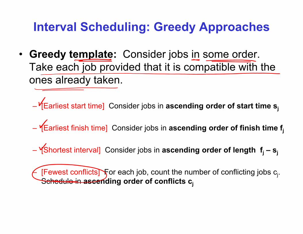
Interval Scheduling: Greedy Approaches
• Greedy template: Consider jobs in some order. Take each job provided that it is compatible with the ones already taken.
– [Earliest start time] Consider jobs in ascending order of start time sj
– [Earliest finish time] Consider jobs in ascending order of finish time fj
– [Shortest interval] Consider jobs in ascending order of length fj – sj
– [Fewest conflicts] For each job, count the number of conflicting jobs cj. Schedule in ascending order of conflicts cj
Interval Scheduling: Greedy Algorithms
• Greedy template: Consider jobs in some order. Take each job provided that it is compatible with the ones already taken.
Counterexample for earliest start time
Counterexample for shortest interval
Counterexample for fewest conflicts
• Consider jobs in increasing order of finish time• Take each job provided that it is compatible with
the ones already taken (i.e., does not overlap or conflict with any previously scheduled jobs)
• Greedy algorithm. Consider lectures in increasing order of start time: assign lecture to any compatible classroom.
Sort intervals by starting time so that s1 s2 ... sn.d 0
for j = 1 to n {if (lecture j is compatible with some classroom k)
schedule lecture j in classroom kelse
allocate a new classroom d + 1schedule lecture j in classroom d + 1d d + 1
}
number of allocated classrooms
Implementation: O(n log n).– For each classroom k, maintain the finish time of the last job added.– Keep the classrooms in a priority queue.
Interval Partitioning: Greedy Analysis• Observation. Greedy algorithm never schedules two
incompatible lectures in the same classroom.
• Theorem. Greedy algorithm is optimal.• Proof.
– Let d = number of classrooms that the greedy algorithm allocates.
– Classroom d is opened because we needed to schedule a job, say j, that is incompatible with all d-1 other classrooms.
– Since we sorted by start time, all these incompatibilities are caused by lectures that start no later than sj.
– Thus, we have d lectures overlapping at time sj + .– Key observation all schedules use d classrooms. ▪
Example of “Achieves the Bound”
Trees
• (Page 141 of PDF; Page 129 of hardcopy: Sidebar)• A tree is connected and acyclic• A tree on n nodes has n - 1 edges• Any connected, undirected graph with |V| - 1 edges is a tree• An undirected graph is a tree if and only if there is a unique
path between any pair of nodes
• Fact about trees: Any two of the following properties imply the third:– Connected– Acyclic– |V| - 1 edges
Minimum Spanning TreeGiven a connected graph G = (V, E) with real-valued edge weights, an MST is a subset of the edges T E such that T is a spanning tree whose sum of edge weights is minimized.
Cayley's Theorem: There are nn-2 spanning trees of Kn
5
23
10 21
14
24
16
6
4
189
7
118
5
6
4
9
7
118
G = (V, E) T, eT ce = 50
can't solve by brute forceSource: slides by Kevin Wayne for Kleinberg-Tardos, Algorithm Design, Pearson Addison-Wesley, 2005.
Greedy MST Algorithms
• Kruskal’s algorithm. Start with T = . Consider edges in ascending order of cost. Insert edge e in T unless doing so would create a cycle.
• Reverse-Delete algorithm. Start with T = E. Consider edges in descending order of cost. Delete edge e from T unless doing so would disconnect T.
• Prim’s algorithm. Start with some root node s and greedily grow a tree T from s outward. At each step, add the cheapest edge e to T that has exactly one endpoint in T.
Source: slides by Kevin Wayne for Kleinberg-Tardos, Algorithm Design, Pearson Addison-Wesley, 2005.
Huffman Codes• How to transmit English text using binary code?• 26 letters + space = alphabet has 27 characters
– 5 bits per character suffices
• Observation #1: Not all characters occur with same frequency– Sherlock Holmes, “The Adventure of the Dancing Men” :
ETAOIN SHRDLU– Suggests variable-length encoding
• Observation #2: Variable-length code should have prefix property– One code word per input symbol– No code word is a prefix of any other code word– Simplifies decoding process
Minimize Wi LiWi = frequency of char iLi = length of codeword for char i
CSE 8, 21, 100, …
Greedy Algorithm: Huffman Coding
• Huffman coding is based on probability (frequency) with which symbols appear in a message
– Goal is to minimize the expected code message length• How it works
– Create a tree root node for each nonzero symbol frequency, with the frequency as the value of the node
– REPEAT• Find two root nodes with smallest value• Create a new root node with these two nodes as
children, and value equal to the sum of the values of the two children
• (Until there is only one root node remaining)
Why Huffman is Optimal• Suppose we have an optimal tree T, where a, b are
siblings at the deepest level, while x, y are the two roots merged by Huffman’s algorithm
• Swap x with a, y with b• Neither swap can increase cost
– x and y have minimum weight– locations of a and b are at the deepest level
T
x
a b
y
Huffman Coding Example
• Example:A E G I M N O R S T U V Y Blank
1 3 2 2 1 2 2 2 2 1 1 1 1 3Frequency:
(Generic Implementation)
• Place the elements into a min heap (by frequency)
• Remove the first two elements from the heap
• Combine these two elements into one
• Insert the new element back into the heap
Symbol:
Huffman Coding Example
Step 1: Step 2:
Step 3: Step 4:
2
A M
2
T U
2
V Y
4
2
V Y
2
A M
2
T U 2
T U
4
N
4
2
V Y
2
A M
Huffman Coding Example
Step 5:
Step 6:
2
T U
4
N
4
2
V Y
2
A M
4
O R
2
T U
4
N
4
2
V Y
2
A M
4
O R
4
S G
Huffman Coding Example
Step 7
Step 8
2
T U
4
N
4
2
V Y
2
A M
5
I E
4
S G
4
O R
2
T U
4
N
5
I E
4
S G
4
O R4
2
V Y
2
A M
7
Huffman Coding Example
• Step 9
5
I E
4
S G
9
4
2
V Y
2
A M
7
2
T U
4
N
4
O R
8
15
Huffman Coding Example
Final tree:
5
I E
4
S G
9
4
2
V Y
2
A M
7
2
T U
4
N
4
O R
8
15240 1
0
0 0 0
0
0 0
0
0
0 0
0
1
1
1
1
1
1
1
1
11
1
E.g., code word for “Y” is “10101”
Sum of internal node values = total weighted pathlength of tree = Wi Li = 4+5+9+2+2+4+7+2+4+4+8+15+24 = 90 (vs. Wi Li = 120 in naïve 5 bit per symbol code)